1. Introduction
Reinforcement learning (RL) and deep reinforcement learning (DRL) are incredibly autonomous and interoperable, i.e., they have many real-time Internet of Things (IoT) applications. RL pertains to a machine learning method based on trial-and-error, which improves the performance by accepting feedback from the environment [
1,
2]. There have been many studies on applying RL or DRL in IoT, which are relevant to a variety of applications, such as energy demand based on the critical load or real-time electricity prices in a smart grid. Robots or smart vehicles using IoT are autonomous in their working environment, wherein they attempt to find a collision-free path from the current location to the target. Regarding the applications of RL or DRL in autonomous IoT, a broad spectrum of technology exists, such as fast real-time decisions made locally in a vehicle or the transmission of data to and from the cloud [
1,
2]. In particular, one of the large issues regarding a real-time fast decision is online learning and decision making based on approximate results from the learning [
1,
2,
3] similar to near-optimal path-planning with respect to real-time criteria. However, the real-time environment might be imprecise, dynamic, and partially non-structured [
1,
2,
3,
4]. Owing to the complexity of online learning and real-time decisions in RL or DRL, Q-learning or a deep Q-network (DQN) has been widely adopted along with some pre-trained [
5] or prior knowledge, such as environmental maps or environmental dynamics [
6]. In [
5], the authors showed that deep Q-learning with transfer learning is significantly applicable in emergency situations such as fire evacuation planning. Their models have shown that an emergency evacuation can benefit from RL because it is highly dynamic, with a lot of changing variables and complex constraints. Prior knowledge can help a smart robot with navigation planning and even obstacle avoidance. Fundamentally, however, little prior knowledge of RL has been presumed.
The approach of the proposed model is similar to that of recent studies [
7,
8], which have applied RL techniques to real-time applications on an online basis and a combination of different algorithms, without prior knowledge. These environments pose more challenges than a simulated environment, such as enlarged state spaces and an increased computational complexity. The primary advantage of RL lies in its inherent power of automatic learning even in the presence of small changes in the real-time environment. Regardless of whether real-time applications with self-learning have become a significant research topic, there have already been some studies based on improved Q-learning or a DQN on the replacement of the complicated parameters, although in approximations and not in actual results [
1,
2]. In [
7], the authors investigated when an optimization is necessary through an online method. In the era of big data, in [
7], a DQN and deep policy gradient (DPG) are proposed to overcome the time consumption required for all possible solutions and to allow the best solution to be chosen. Moreover, the authors showed that their models are capable of generalization and exploitation and minimize the energy consumption or cost in newly encountered situations [
7]. In [
8], the authors demonstrated how a different mixing of off-policy gradient estimates with on-policy samples contribute to improvements in the empirical performance of a DRL. However, recent research [
1] has shown that a DRL is confronted with situations that differ in minor ways from those upon which the DRL was trained, indicating that solutions to DRLs are often extremely superficial. Most of these studies require the state spaces of the smart grid to be well-organized, notwithstanding that real applications take place in real value vectors of the state spaces, which are continuous and large in scale [
1]. Thus, using only Q-learning with complicated reward functions in real applications can lead to larger issues, such as the curse of dimensionality [
1,
7]. In terms of the approximation of a value function, a generalization in RL can cause a divergence in the case of bootstrapped value updates [
9]. Therefore, we are devoted to determining and thoroughly understanding why and when an RL is able to work well. The design is also inspired by recent studies [
2,
9,
10,
11] that provide a better understanding on the role of online and offline environments in RL, which are characterized by an extremely high observation dimensionality and infinite-dimensional state spaces. Hausknecht and Stone [
9] indicated that mixing an off-policy Q-learning of online TD updates with offline MC updates provides an increased performance and stability for a deep deterministic policy gradient. However, Hausknecht and Stone [
9] showed slow learning for deep Q-learning. In addition, Xu et al. [
10] proposed deep Sarsa and Q-networks, which are combined with both on-policy Sarsa and off-policy Q-learning in online learning. Off-policy Q-learning is considered better than on-policy Sarsa in terms of the local minima in online learning. However, Q-learning also suffers from a high bias estimate because the estimate is never completely accurate [
3]. Wang et al. [
11] also combined Sarsa and Q-learning but utilized some information regarding a well-designed reward until the maximum time is reached. As such, their study [
11] necessitated the full storage for the entire episode as a worst case. By contrast, the proposed model does not consider a well-designed reward for optimization, thereby making it different from the research by Wang et al. Remarkably, Amiranashvili et al. [
2] demonstrated that, in a representative online learning, the temporal difference (TD), is not always superior to a representative offline learning, i.e., a Monte Carlo (MC) approach.
In this study, we exploit a combination of an offline learning MC approach and off-policy Q-learning and an on-policy state-action–reward-state-action (Sarsa) of online learning TD. The purpose of this combination is to achieve a reasonable performance and stability with reply memories and updates to a target network [
12] while ensuring a real-time online learning criterion in the environments. By using the DQN, which is the de facto standard, Q-estimates are computed using the target network, which can provide older Q-estimates, with a specific bias limiting the generalization but achieving a more stable network instead. In RL, bias and variance indicates how well the RL signals reflect the true rewards in the environment. A combination of online and offline environments is applied for a bias-variance tradeoff [
13]. Previous studies [
8,
14] have handled the issues involved in balancing bias and variance. The most common approaches are to reduce the variance of an estimate while keeping the bias unchanged. The baselines of such studies [
8,
14] are of the policy gradient [
15], which utilizes an actor, who defines the policy, and a critic, who provides a more reduced variance reward structure to update the actor.
Herein, we consider DQN, the de facto standard, and Q-learning with a ε-greedy algorithm for the balance of exploration and exploitation, which is easily applicable to more general cases and is a simple but powerful strategy for the challenge of bias–variance tradeoff—a crucial element in several RL components. This study aims to bridge the gap between theory and practice using a simple RL strategy. Therefore, we rely on the “baseline” of the balance in offline MC and online TD with off-policy Q-learning and on-policy Sarsa in a real-time environment. Based on these considerations, we propose a random probability that determines whether to use an offline or online environment during the learning process. The initial value of probability δ is δini. The value of δini is set to 1.0; therefore, the proposed algorithm will use offline learning with higher probability during the initial stage. For random probability δ, each step is decreased by Δδ until δfin = 0.01. Consequently, the proposed algorithm will more likely utilize online learning with an on- and off-policy during the late stage. The algorithm is based on a simple and random method with probability δ, and it has facilitated better prediction by the agent in several cases. Therefore, as training of the agent progresses, a complete episode for offline learning is not required.
Through this study, we show that merely using only a DQN by balancing offline and online environments with an on- and off-policy achieves a satisfactory result. We demonstrate the capability of the proposed model and its suitability for RL in an autonomous IoT for achieving a bias–variance trade-off. The aforementioned contributions are significant because several researchers have based their studies on complex function approximations with deep neural networks. In the simulations using control problems such as a cart-pole balancing, mountain-car, and lunar-lander from the OpenAI Gym [
16], we demonstrated that in simple control task such as a cart-pole and mountain-car, merely the balance of online and offline environments without an on- and off-policy achieves satisfactory results. However, in complex tasks such as a lunar-lander or the cart-pole and mountain-car with qualified upper bound, the results provide direct evidence of the effectiveness of the combined method for improving the convergence speed and performance. The proposed algorithm initially chooses a gradual balance from an offline environment, followed by online with on- and off-policy towards the end of the application, with a simple and random probability. Furthermore, we attempt to demonstrate the superiority of this algorithm over other technique by comparing it with the classic DQN, DQN with MC, and DQN with Sarsa. The proposed algorithm aims to achieve a significantly lightweight version of a random balance of the probability, and is worth consideration in most real-time environments.
2. Background
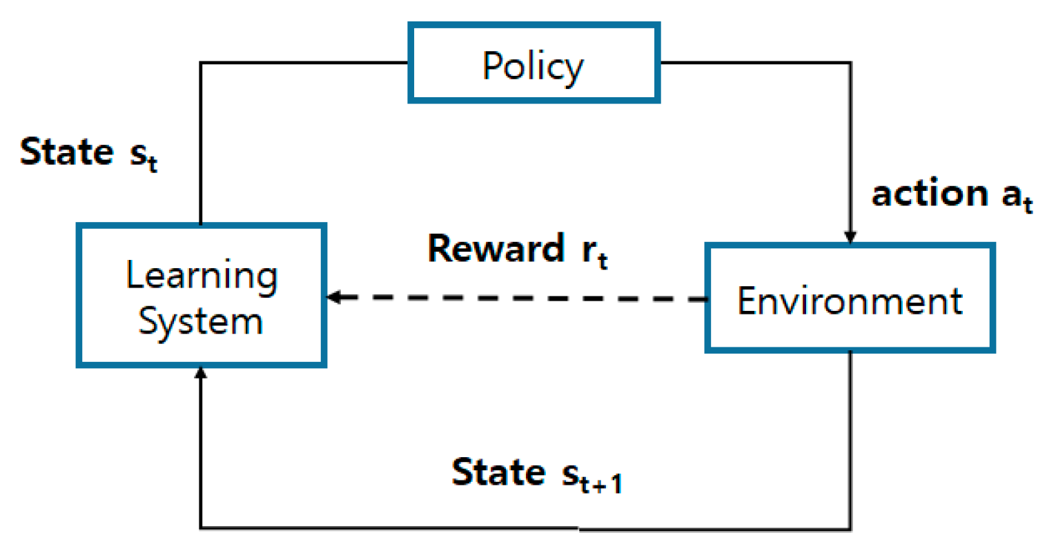
The standard structure of the RL [
17,
18,
19] is given in
Figure 1. The environment and agent of the learning system interact continuously. The agent, based on the policy, selects an action a
t in the current state s
t. The environment will then supply a reward to the agent based on the action a
t, and create a new situation, s
t+1. In the environment, the state s
t, the action a
t, the reward r
t+1, the new state s
t+1, and the new action a
t+1 are presented in a circular form. RL attempts to teach the agent how to improve the action, when placed in an unknown environment, by acquiring the near-optimal Q-values that achieve the best results for all states. The agent takes advantage of the rewards given by the environment after selecting an action in every state to update the Q-values for a convergence of optimality. The constant issue of a trade-off between exploration and exploitation in the unknown environment in an RL algorithm has yet to be addressed. On the one hand, choosing the action with the best-estimated value implies that the agent exploits its current knowledge. On the other hand, choosing one of the other actions implies that the agent explores how to improve its estimate of the values of such actions. The exploitation maximizes the reward system in the short term. However, it does not guarantee a maximization of the accumulated reward in the long run. As such, although the exploration reduces the short-term benefits of the total rewards, it produces the maximum reward in the long run. This is because, after the agent has explored the actions at random, allowing the agent to check for better alternatives, it can begin to exploit them. It must be noted that exploitation and exploration are mutually exclusive. Hence, the agent cannot perform both exploration and exploitation in one selection. Therefore, it is fundamentally essential to balance the exploration and exploitation for the convergence of the near-optimal value functions. The most common algorithm for balancing this trade-off of exploration and exploitation is the ε-greedy algorithm. In this algorithm, the action with the maximally estimated value is called the “greedy action,” and the agent usually exploits its current knowledge by choosing this so-called greedy action. However, there are other chances of probability ε for the agent to explore under a random selection, i.e., “non-greedy actions.” This type of action selection is called a ε-greedy algorithm [
17,
18,
19].
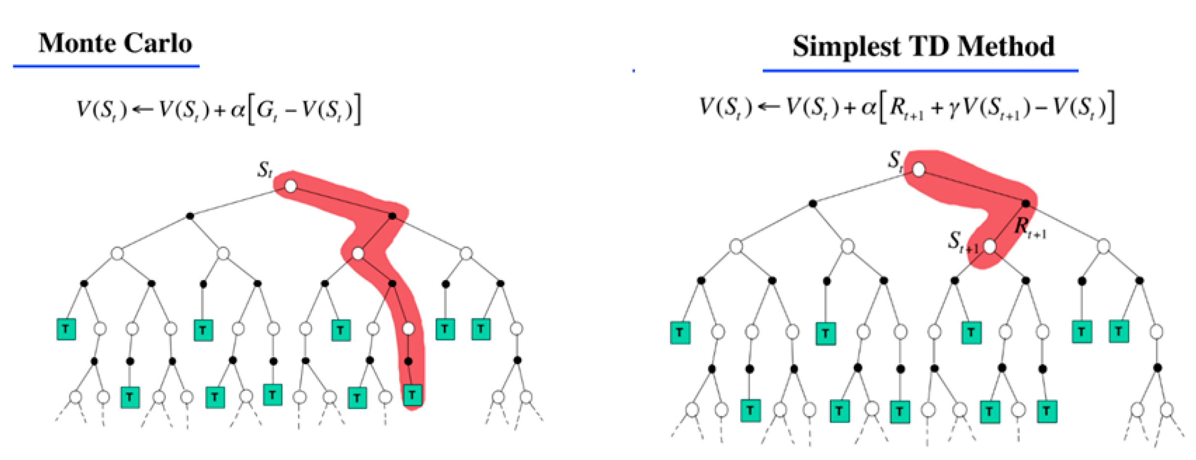
Furthermore, two different approaches, MC and TD, are applied when dealing with the trade-off between online and environments offline for determining the Q-value functions in RL [
17]. TD can learn before knowing the final outcome. Thus, TD can learn online after every step. However, MC can only learn from complete sequences. Thus, MC learning is offline.
Figure 2 shows a significant difference between MC and TD. In
Figure 2, V(S
t) is the value fuction at S
t and G
t is the total discounted reward. α is the learning rate and γ is the discount factor. R
t+1 + γV(S
t) is the estimated return, also known as the TD-target, and [R
t+1 + γV(S
t) − V(S
t)] is TD-error. In addition,
Figure 3 shows a first-visit MC policy evaluation [
17].
Among the most common TD algorithms are Sarsa, which is an on-policy, and Q-learning, an off-policy. There are two types of policy learning methods in RL: on-policy and off-policy. On-policy learns on the job, which means it evaluates or improves the policy that is used to make the decisions. By contrast, off-policy evaluates one target policy, while following another behavior policy. TD methods allow learning directly from the previous experience, do not require any model of the environment, ascertain convergence for near-optimal performance, and are easy to implement. For these reasons, TD methods have been widely adopted since researchers first started using RL algorithms. The Sarsa algorithm was proposed by Rummery and Niranjan [
20]. The Sarsa algorithm estimates the value of Q(s
t, a
t) by applying a
t in state s
t according to the updated formula
This update can be performed after every transition from a non-terminal state s
t. Here, Q(s
t+1, a
t+1) is determined as zero if s
t+1 is terminal. Every element of the quintuple event (s
t, a
t, r
t+1, s
t+1, a
t+1) is used in the updated Formula (1), which is a transition from a pair of one state s
t and action a
t to the next. Thus, this quintuple leads to the name Sarsa. The Sarsa algorithm is shown in
Figure 4.
Morever, the most popular TD, Q-learning, which is an off-policy proposed by Watkins and Dayan, is one of the most important RL algorithms [
21]. Q-learning is determined by
where α is the learning rate, γ is the discount factor, and r
t+1 is the immediate reward received from the environment by taking action a
t in state s
t at the moment of time t. The Q-learning algorithm is given in
Figure 5. The difference between Sarsa and Q-learning is the TD-target, which is mentioned above. The TD-target, R+ γQ(S’, A’) in Sarsa means “Update the current Q value with the immediate reward and the Q value of the next action”. However, the TD-target, R+ γmax
aQ(S’, a) in Q-learning means “an next action is chosen using behavior policy. But, the alternative successor action is considered.” Therefore, Q-learning is off-policy, which means it will “Evaluate target policy while following behavior policy”.
Sarsa is actually an enhancement of Q-learning in terms of fast convergence. In other words, Sarsa allows the agent to learn faster than normal. Apart from Sarsa, other studies have focused on improving the learning performance in Q-learning [
17,
18,
19].
DQN is a well-known, model-free RL algorithm attributed to discrete action spaces. In DQN [
18,
19], we construct a DNN, Q, which approximates Q* and is greedily defined as π
Q(s) = argmax
a∈AQ(s,a) [
18,
19]. This is a ε-greedy policy with probability ε that takes the action π
Q(s) with probability 1-ε. Each episode uses the ε-greedy policy following Q as an approximation of a DNN. The tuples (s
t, a
t, r
t, s
t+1) are stored in the replay buffer, and each new episode is configured to neural network training [
18,
19]. The DNN is trained using the gradient descent of random episodes on a loss function, encouraging Q to follow the Bellman equation [
17]. The tuples are sampled from the replay buffer of random episodes. The target network y
t is computed using a separate neural network that changes more slowly than the main deep neural network to optimize the process stability. The weights of the target network are set to the current weights of the main deep neural network. The DQN algorithm [
18,
19] is presented in
Figure 6. The maximum action a
t is selected by Q*((s
t), a; θ) of DNN with the probability 1-ε. The TD-target, y
j is r
j + γmax
a’Q(Φ
j+1, a’; θ) and TD-error is y
j − Q(Φ
j, a
j; θ). The DNN performs a gradient descent on the TD-error.
4. Evaluation and Results
We augmented a full episode of transition tuples into the replay memory Ω and compute backward the tuples for online MC and in D for TD, where all samples are bootstrapped. With the probability δ1, the targets present a way for a bias–variance tradeoff between online MC and offline TD. Moreover, with the probability δ2, the proposed algorithm makes the Q-value estimates reduce the overestimates and not diverge to infinity as the updates continually grow. We selected a few classic control tasks in OpenAI Gym [
16] for the comparisons of the proposed offline-online in DQN algorithm with DQN, DQN with MC, and DQN with Sarsa. We implemented these four algorithms with PYTHON Tensorflow and Keras [
25,
26]. First, we compared the offline–online approaches in the DQN algorithm with DQN, DQN with MC, and DQN with Sarsa on a Cart-Pole [
27], the most used control task for RL algorithms. Next, we conducted experiments on MountainCar [
28]. Finally, we tested the offline–online approach using the DQN algorithm on LunarLander [
29], a more complex task than Cart-Pole and MountainCar. We exploited a function approximation, such as an artificial neural network, for the four algorithms. For the experimental setup, the first dense layer has four inputs, 24 outputs, and a ReLU activation function [
30]. The second dense layer has 24 inputs, 24 outputs, and ReLU. The third has 24 inputs, 24 outputs, and a linear function. The loss of the model is a mean square error, and the optimizer is an adaptive moment estimation (Adam) [
31]. For the hyper-parameters, the discount factor, γ = 0.95, the learning rate, α = 0.001, ε_max = 1.0, ε_min = 0.01, ε_decay = 0.995, the bootstrapped Mini-Batch = 64, and the target network parameter update, C = 300. For the offline-online in DQN, the probability δ1 for offline and online environments are as follows: The initial value of probability δ1 is δ1
ini = 0.99. For probability δ1, each step is decreased by Δδ1 until it equals δ1
fin = 0.01, where Δδ1 = δ1
ini − (δ1
ini − δ1
fin)/N, and N refers to the total number of episodes. Likewise, the probability δ2 for an on- and off-policy are as follows: The initial value of probability δ2 is δ2
ini = 0.99. For probability δ2, each step is decreased by Δδ2 until it equals δ2
fin = 0.01, where Δδ2 = δ2
ini − (δ2
ini − δ2
fin)/N, where N refers to the training steps.
4.1. Cart-Pole Balancing
In Cart-Pole [
27], there are four observations and two discrete actions, as shown in
Figure 7.
A pole is attached to a cart, which goes back and forth from left to right. The pole starts upright. The goal is to not fall over when increasing and decreasing the velocity of the cart. A reward of +1 is considered by the environment for every step when the pole remains upright until the next action is terminated. When the episode is terminated, the angle of the pole is between −12° and +12°, the cart position is between −2.4 and +2.4, or the length of the episode is greater than 200. It is considered solved when the average reward is greater than or equal to 195.0 over 100 consecutive runs [
27].
Figure 8 shows the average rewards of the four algorithms, DQN, DQN with Sarsa, DQN with MC, and the proposed DQN with MC and Sarsa on Cart-Pole [
27]. From these results, we can observe that DQN with only offline MC and the proposed DQN with MC and Sarsa have guaranteed better rewards and converged sooner in the final goal than the other two algorithms. This might indicate that the proposed algorithm can work without an on-policy TD or Sarsa. However, Cart-Pole balancing is simpler than the other tasks.
4.2. Mountain Car
For the MountainCar [
28], there are two observations and three discrete actions, as shown in
Figure 9.
A car goes back and forth between a “left” mountain and a “right” mountain. The goal is to drive up the “right” mountain. The car is not strong enough to go up the “right” mountain without building up momentum, however. Thus, it goes back and forth without a break to create the momentum. A reward of −1 is given for every step when the position is reached at the half-point between the “left” and “right” mountains. The episode is terminated if a 0.5 position of the height of the mountain is reached, or the number of iterations is more than 200. It is considered solved when it obtains an average reward of +110.0 over 100 consecutive runs.
Figure 10 shows the average rewards of the four algorithms, DQN, DQN with Sarsa, DQN with MC, and the proposed DQN with MC and Sarsa on MountainCar [
28]. From these results, we can observe that DQN with only offline MC and the proposed DQN with MC and Sarsa have guaranteed improved rewards similar to the results of Cart-Pole balancing in
Figure 8. The results show that only the balance in offline MC and online Q-learning in DQN, without the balance in off-policy Q-learning and on-policy Sarsa, might work in both Cart-Pole and MountainCar.
4.3. LunarLander
In the LunarLander [
29], there are three observations and four discrete actions, as indicated in
Figure 11. LunarLander as a Box2D-based game was developed by Atari. The landing pad is at the coordinates (0, 0). An approximately 100 to 400 point reward is given by the environment from the top to the landing pad and at zero speed. If the lander moves away from landing pad, the reward is taken away. When the episode is terminated if the lander crashes, then the agent receives −100 or sits down, and then it receives +100. If each leg contacts the ground, it receives +10. In addition, it is possible to land outside the landing pad. It is considered solved when it obtains an average reward of 200 over 100 consecutive runs.
Figure 12 shows the average rewards of four algorithms: DQN, DQN with Sarsa, DQN with MC, and the proposed DQN with MC and Sarsa on LunarLander [
29]. From these results, we can see that the proposed DQN with MC and Sarsa achieves the most stable performance for LunarLander, which is more complex than Cart-Pole or MountainCar. However, the results show that our proposed algorithm and DQN with MC achieved a better performance. Thus, we attempt to make more comparisons with only the proposed algorithm and DQN with an MC based on the environments with some time-constraints. The results are described in
Section 4.4.
4.4. Cart-Pole and MountainCar with Qualified Upper Bound
The maximum episode length of Cart-Pole is 500. For a better comparison of the solutions, we consider a few requirements between only DQN with MC and the proposed offline–online in DQN because the two algorithms show similar performances in Cart-Pole and MountainCar but not in LularLander. The first reason for this is that they receive a reward of −100 when they fall down prior to the maximum length of the episode. The other is that, if the average reward is more than 490 or equal to 500 over 100 consecutive runs, then the loop is terminated. These time constraints in these comparisons are based on the previous implementation [
32], which suggests more restrictive time conditions. Moreover, based on empirical results, we adjust a small parameter between off-policy Q-learning and on-policy Sarsa. We followed the strategies of [
10] between balancing Q-learning and Sarsa. However, in the experiment in this section, we change the parameter slightly, i.e., if r + 1 is between zero and a small constraint, which is selected based on many empirical trials, then we follow the immediate policy. The results of offline–online balance use in DQN show that Q-value divergence in the constraints is preventable.
Figure 13,
Figure 14 and
Figure 15 indicate that offline–online balance use in DQN is worth considering for simple control tasks, such as Cart-Pole. We evaluated only 100 rounds owing to the simple environment.
In MountainCar, we used the phrase “Car has reached the goal” in each round for better comparisons between the proposed algorithm and DQN with MC. It is considered solved when it obtains an average reward of +110.0 over 100 consecutive runs. In addition, we set the reward +150 to “Car has reached its goal.” We check how many times we can use “Car has reached the goal” in a limited number of runs. These qualified constraints in this comparisons are based on the previous implementation [
33].
Figure 16 shows the proposed algorithm uses “Car has reached the goal” 42 times, while DQN with MD uses it 23. They show that the number of “Car has reached the goal” outputs of the proposed algorithm is higher than that obtained by DQN with MC. Under the strict constraints for comparisons of qualification, we demonstrated that the algorithm learns slightly faster than DQN with MC and can balance out the bias–variance trade-off during the training process. It is natural that if we use a transferred model, such as in [
5], the proposed model could become faster during the training. However, the pre-trained model in [
5] could fail in a variety of minor perturbations [
3], specifically in a real-time environment. These results might indicate that the offline–online in DQN can check the performance in terms of the balance in offline MC and online TD. Moreover, it can provide better results when it comes to constrains such as real-world settings.


