Improving the Results of the Earned Value Management Technique Using Artificial Neural Networks in Construction Projects
Abstract
1. Introduction
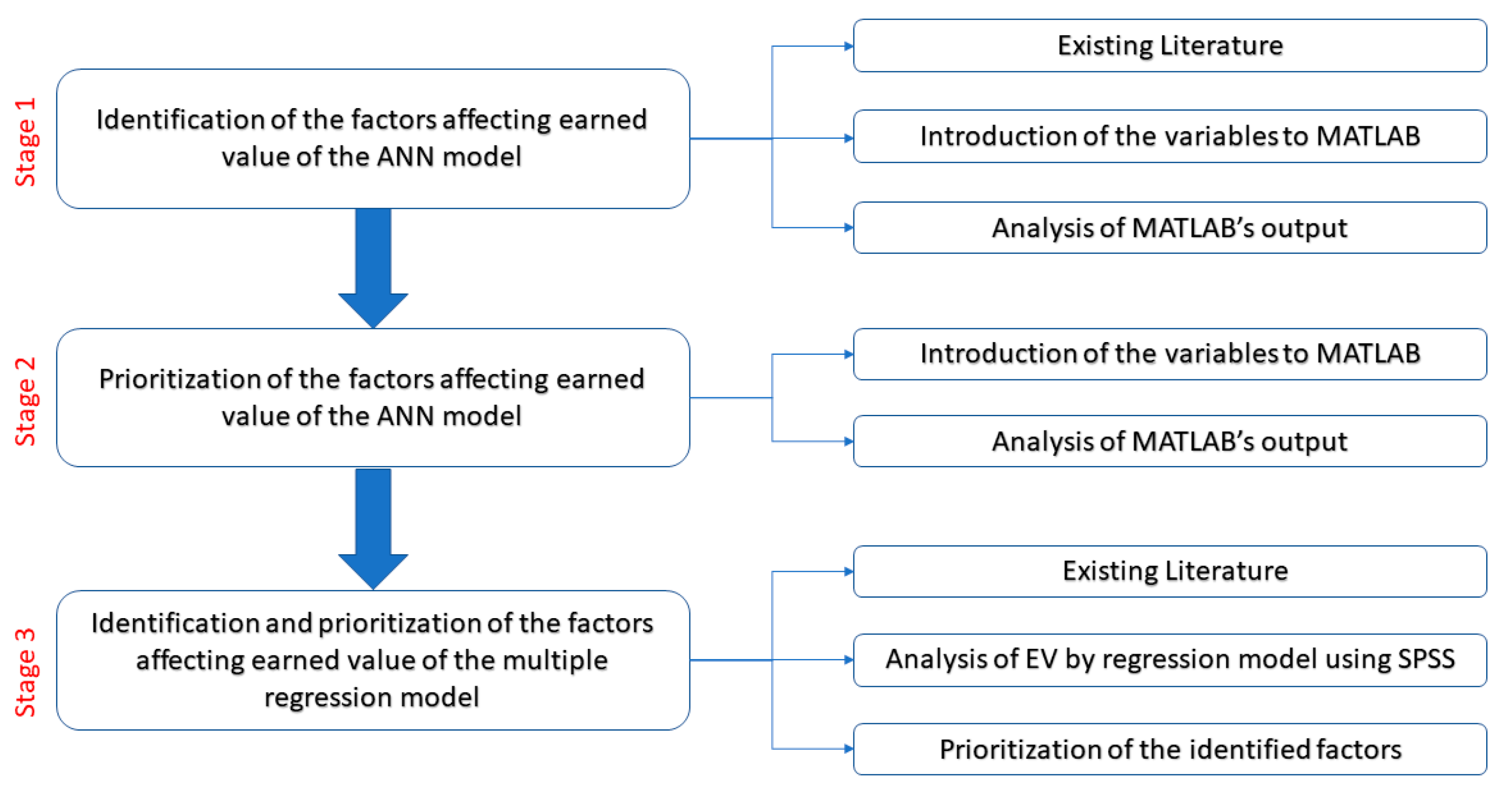
2. Methodology
2.1. Predicting Earned Value Using Artificial Neural Network
2.1.1. Input Data
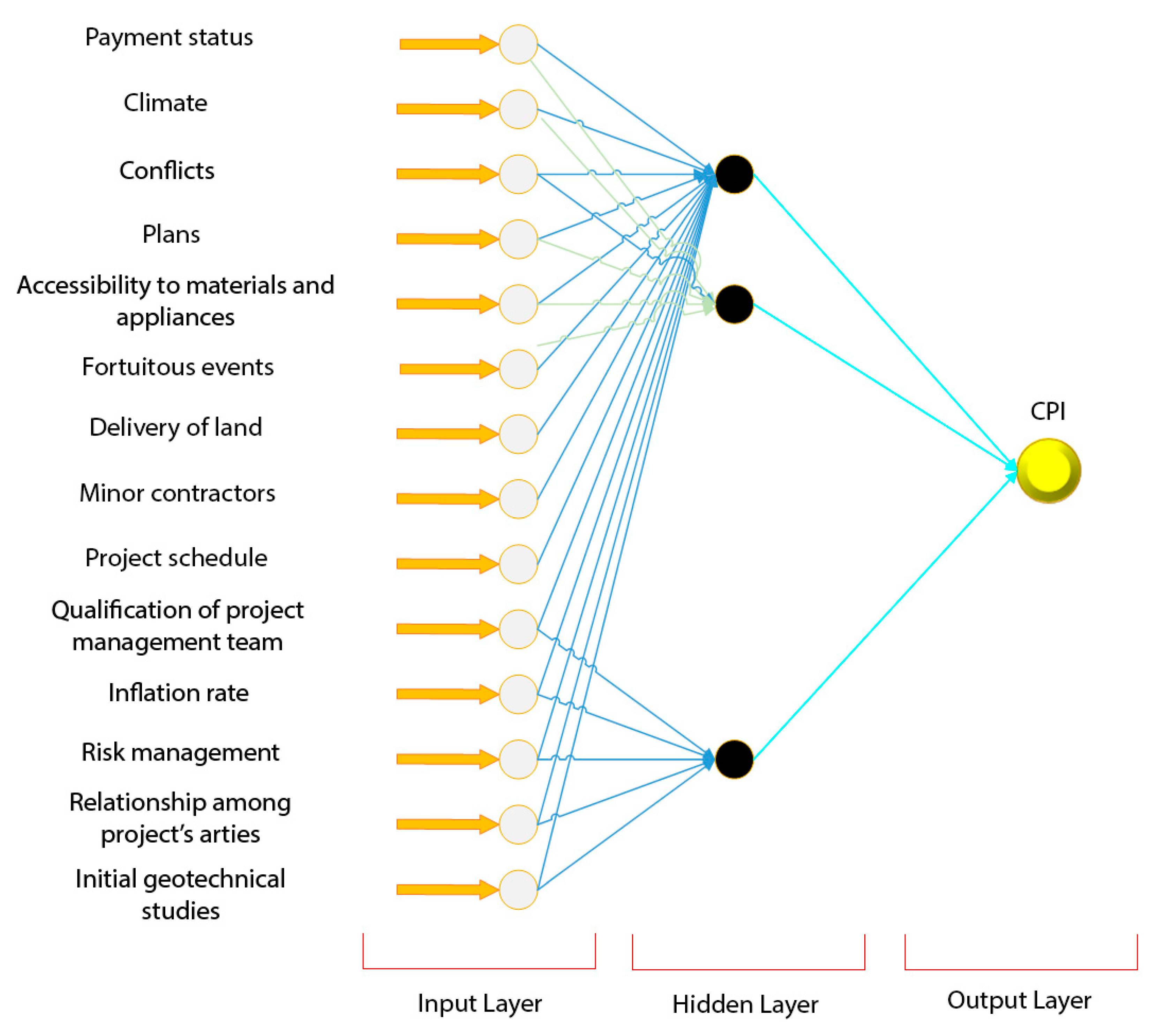
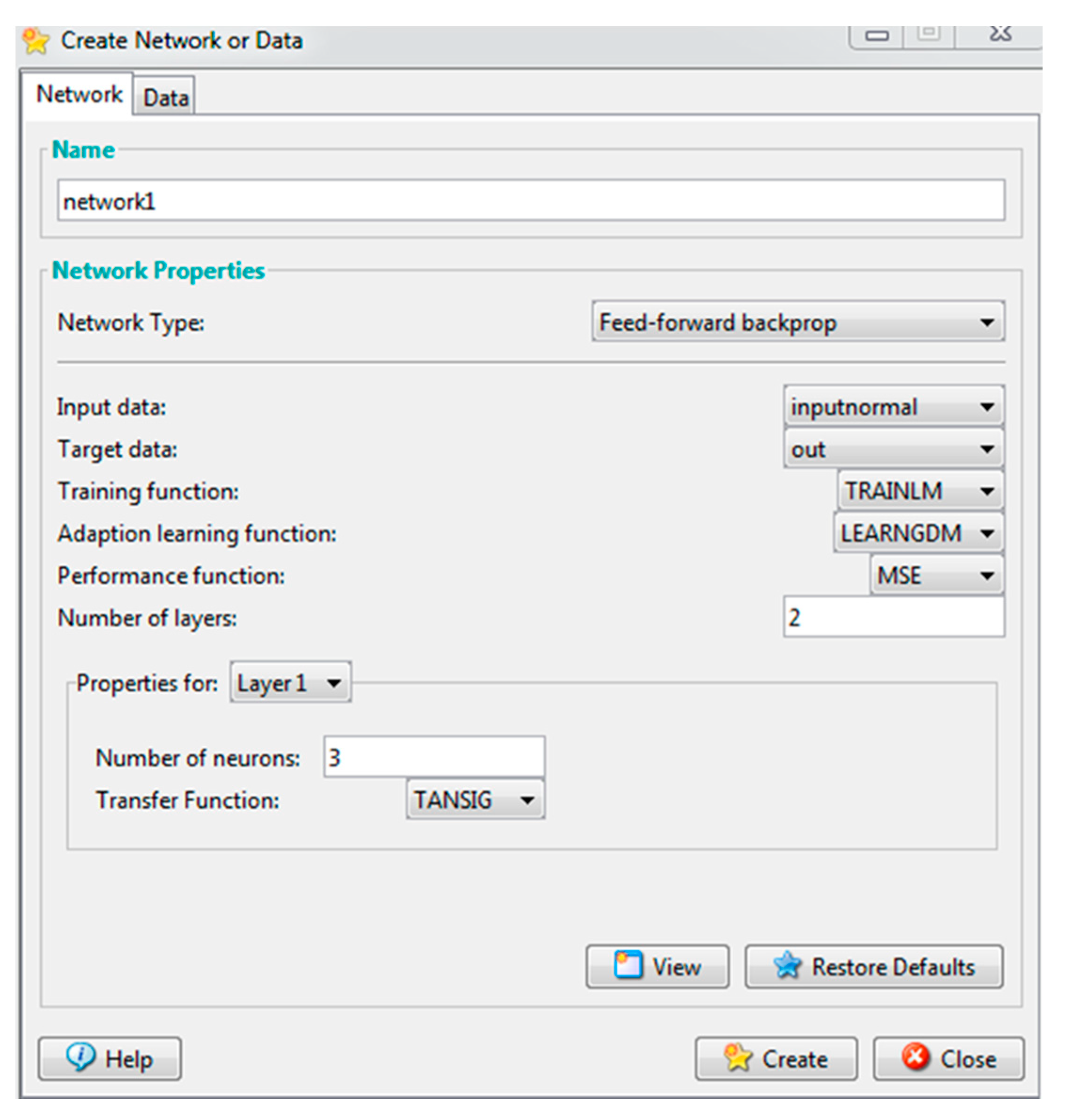
2.1.2. Architecture of the Network
2.2. Determination and Prioritization of Factors Using ANN
2.3. Earned Value Prediction Using Multiple Regression Method
2.4. Data Collection
3. Results and Discussion
3.1. Predicting Earned Value Using Artificial Neural Network
3.1.1. Gathering the MLP Network’s Data
3.1.2. Normalizing Data
3.1.3. Determining Hidden Layers of ANN
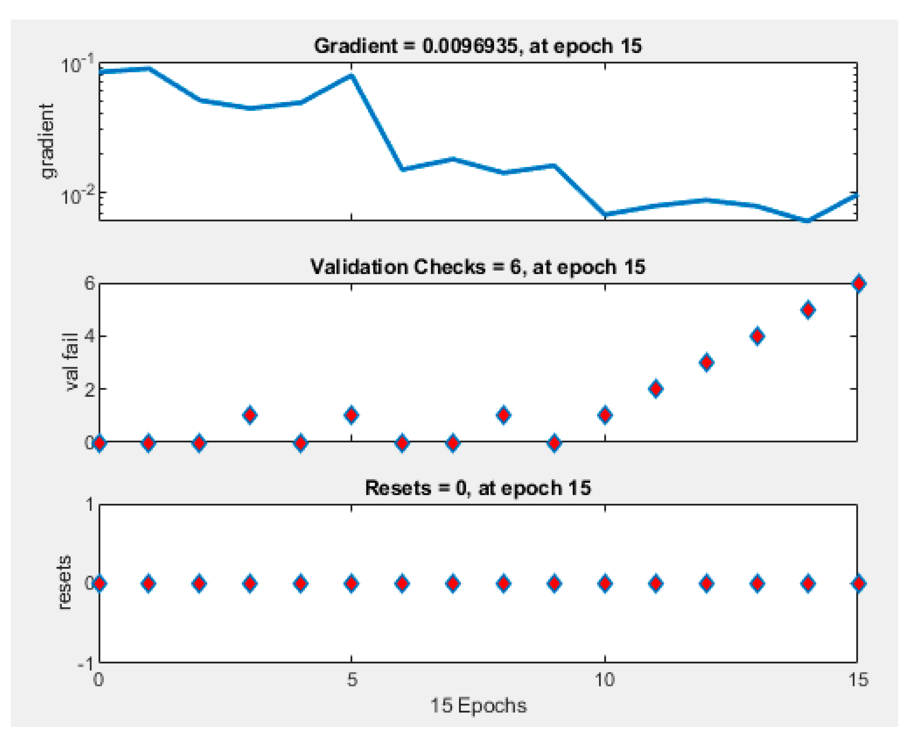
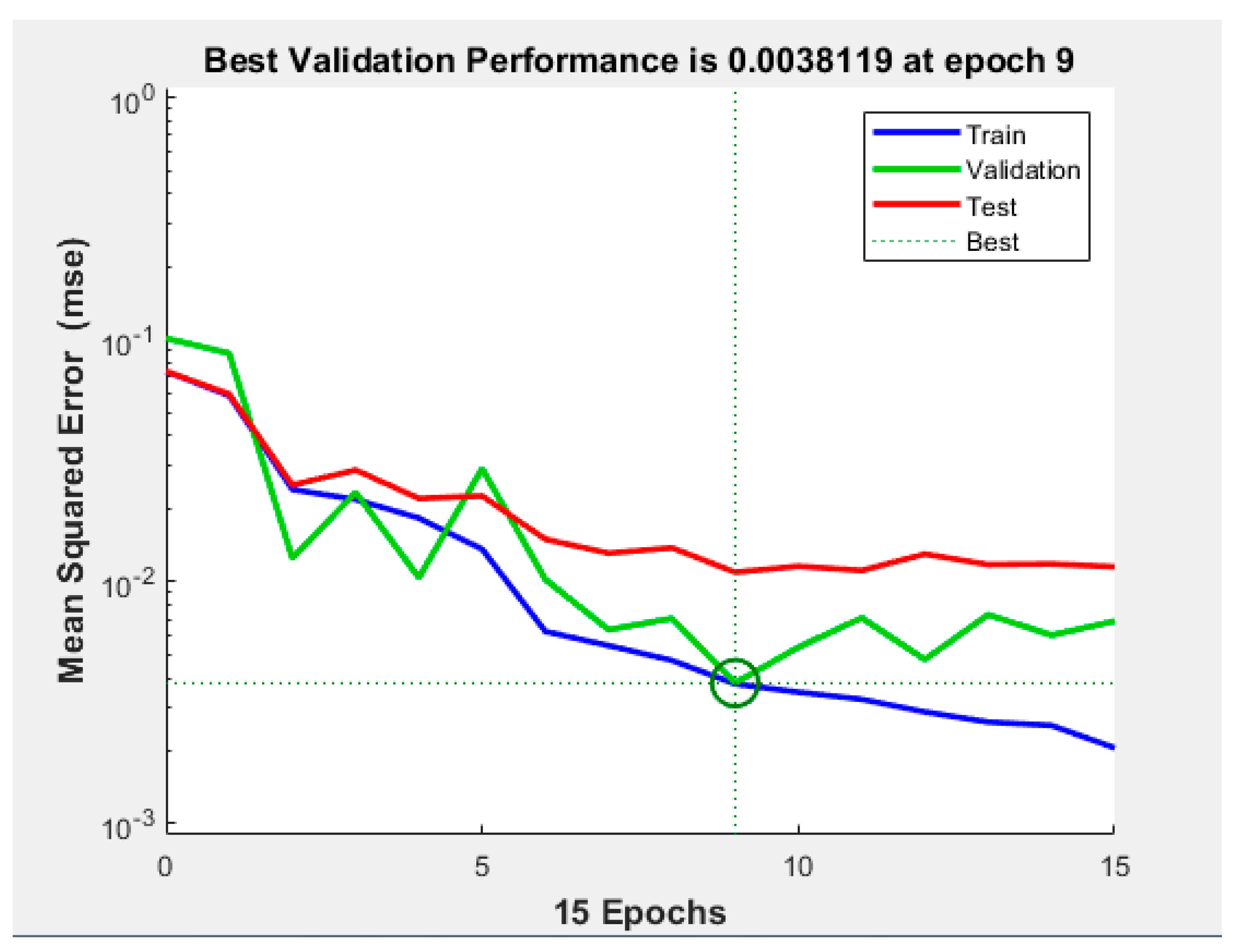
3.1.4. Training of the ANN
3.2. Determination and Prioritization of Factors Affecting Earned Value in the ANN
3.3. Determination and Prioritization of Factors Affecting Earned Value Using Multiple Regression Method and Comparison with the ANN Model for Data Validation
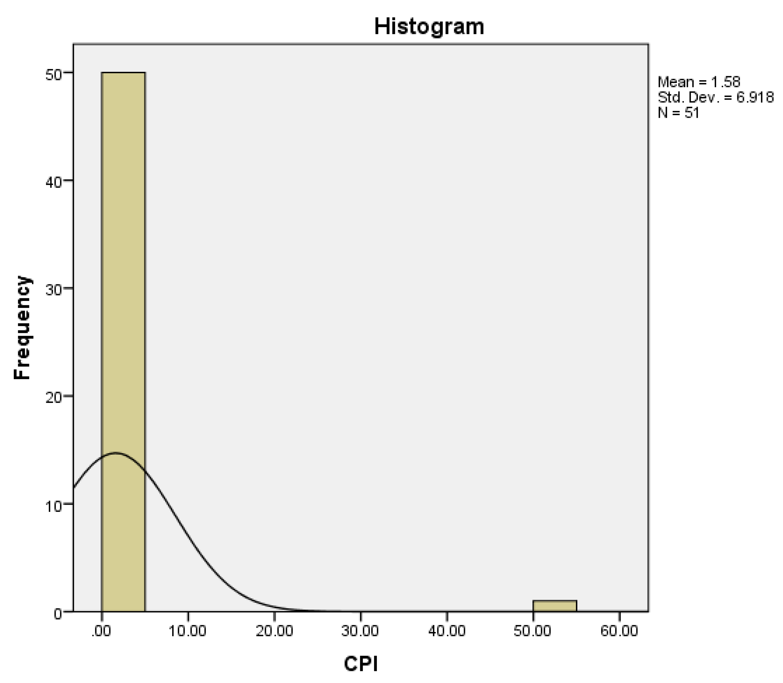
3.3.1. Investigating the Condition of Using Multiple Regression Analysis
3.3.2. Analysis of Multiple Regression Model
4. Conclusions
Author Contributions
Funding
Conflicts of Interest
References
- Mahalakshmi, G.; Rajasekaran, C. Early cost estimation of highway projects in India using artificial neural network. In Sustainable Construction and Building Materials Lecture Notes in Civil Engineering; Das, B., Neithalath, N., Eds.; Springer: Singapore, 2019; Volume 25, pp. 659–672. [Google Scholar]
- Wideman, R.M. Cost Control of Capital Projects and the Project Cost Management System Requirements: A Handbook for Owners, Architects, Engineers, and All Those Involved in Project Management of Constructed Facilities; AEW Services, BiTech Publishers: Richmond, BC, Canada, 1995. [Google Scholar]
- Al-Zwainy, F.M.; Aidan, I.A.-A. Forecasting the cost of structure of infrastructure projects utilizing artificial neural network model (highway projects as case study). Indian J. Sci. Technol. 2017, 10, 1–12. [Google Scholar] [CrossRef]
- Turochy, R.E.; Hoel, L.A.; Doty, R.S. Highway Project Cost Estimating Methods Used in the Planning Stage of Project Development; Virginia Transportation Research Council: Charlottesville, VA, USA, 2001. [Google Scholar]
- Sodikov, J. Cost estimation of highway projects in developing countries: Artificial neural network approach. J. East. Asia Soc. Transp. Stud. 2005, 6, 1036–1047. [Google Scholar]
- Czernigowska, A. Earned value method as a tool for project control. Bud. Archit. 2008, 3, 15–32. [Google Scholar]
- Anbari, F.T. Earned value project management method and extensions. Proj. Manag. J. 2003, 34, 12–23. [Google Scholar] [CrossRef]
- Koke, B.; Moehler, R.C. Earned Green Value Management for Project Management: A systematic review. J. Clean. Prod. 2019, 230, 180–197. [Google Scholar] [CrossRef]
- Bryde, D.; Unterhitzenberger, C.; Joby, R. Conditions of success for earned value analysis in projects. Int. J. Proj. Manag. 2018, 36, 474–484. [Google Scholar] [CrossRef]
- Colin, J.; Vanhoucke, M. A comparison of the performance of various project control methods using earned value management systems. Expert Syst. Appl. 2015, 42, 3159–3175. [Google Scholar] [CrossRef]
- Kerkhove, L.-P.; Vanhoucke, M. Extensions of earned value management: Using the earned incentive metric to improve signal quality. Int. J. Proj. Manag. 2017, 35, 148–168. [Google Scholar] [CrossRef]
- Abdi, A.; Taghipour, S.; Khamooshi, H. A model to control environmental performance of project execution process based on greenhouse gas emissions using earned value management. Int. J. Proj. Manag. 2018, 36, 397–413. [Google Scholar] [CrossRef]
- Sutrisna, M.; Pellicer, E.; Torres-Machi, C.; Picornell, M. Exploring earned value management in the Spanish construction industry as a pathway to competitive advantage. Int. J. Constr. Manag. 2020, 20, 1–12. [Google Scholar] [CrossRef]
- De Andrade, P.A.; Martens, A.; Vanhoucke, M. Using real project schedule data to compare earned schedule and earned duration management project time forecasting capabilities. Autom. Constr. 2019, 99, 68–78. [Google Scholar] [CrossRef]
- Kulkarni, P.; Londhe, S.; Deo, M. Artificial neural networks for construction management: A review. J. Soft Comput. Civ. Eng. 2017, 1, 70–88. [Google Scholar]
- Adeli, H.; Yeh, C. Perceptron learning in engineering design. Comput. Aided Civ. Infrastruct. Eng. 1989, 4, 247–256. [Google Scholar] [CrossRef]
- Adeli, H. Neural networks in civil engineering: 1989–2000. Comput. Aided Civ. Infrastruct. Eng. 2001, 16, 126–142. [Google Scholar] [CrossRef]
- Peško, I.; Mučenski, V.; Šešlija, M.; Radović, N.; Vujkov, A.; Bibić, D.; Krklješ, M. Estimation of costs and durations of construction of urban roads using ANN and SVM. Complexity 2017, 2017, 2450370. [Google Scholar] [CrossRef]
- Albino, V.; Garavelli, A.C. A neural network application to subcontractor rating in construction firms. Int. J. Proj. Manag. 1998, 16, 9–14. [Google Scholar] [CrossRef]
- Leung, A.W.; Tam, C.; Liu, D. Comparative study of artificial neural networks and multiple regression analysis for predicting hoisting times of tower cranes. Build. Environ. 2001, 36, 457–467. [Google Scholar] [CrossRef]
- Cheung, S.O.; Wong, P.S.P.; Fung, A.S.; Coffey, W. Predicting project performance through neural networks. Int. J. Proj. Manag. 2006, 24, 207–215. [Google Scholar] [CrossRef]
- Vouk, D.; Malus, D.; Halkijevic, I. Neural networks in economic analyses of wastewater systems. Expert Syst. Appl. 2011, 38, 10031–10035. [Google Scholar] [CrossRef]
- Mučenski, V.; Trivunić, M.; Ćirović, G.; Peško, I.; Dražić, J. Estimation of recycling capacity of multi-storey building structures using artificial neural networks. Acta Polytech. Hung. 2013, 10, 175–192. [Google Scholar]
- Chaphalkar, N.; Iyer, K.; Patil, S.K. Prediction of outcome of construction dispute claims using multilayer perceptron neural network model. Int. J. Proj. Manag. 2015, 33, 1827–1835. [Google Scholar] [CrossRef]
- Golnaraghi, S.; Zangenehmadar, Z.; Moselhi, O.; Alkass, S. Application of artificial neural network (s) in predicting formwork labour productivity. Adv. Civ. Eng. 2019, 2019, 5972620. [Google Scholar] [CrossRef]
- Tijanić, K.; Car-Pušić, D.; Šperac, M. Cost estimation in road construction using artificial neural network. Neural Comput. Appl. 2020, 32, 9343–9355. [Google Scholar] [CrossRef]
- Casilari-Perez, E.; García-Lagos, F. A comprehensive study on the use of artificial neural networks in wearable fall detection systems. Expert Syst. Appl. 2019, 138, 112811. [Google Scholar] [CrossRef]
- Kim, H.-J.; Jo, N.-O.; Shin, K.-S. Optimization of cluster-based evolutionary undersampling for the artificial neural networks in corporate bankruptcy prediction. Expert Syst. Appl. 2016, 59, 226–234. [Google Scholar] [CrossRef]
- Kocadagli, O.; Langari, R. Classification of EEG signals for epileptic seizures using hybrid artificial neural networks based wavelet transforms and fuzzy relations. Expert Syst. Appl. 2017, 88, 419–434. [Google Scholar] [CrossRef]
- Kwon, H.-B.; Lee, J.; Davis, K.N.W. Neural network modeling for a two-stage production process with versatile variables: Predictive analysis for above-average performance. Expert Syst. Appl. 2018, 100, 120–130. [Google Scholar] [CrossRef]
- Bandara, K.; Bergmeir, C.; Smyl, S. Forecasting across time series databases using recurrent neural networks on groups of similar series: A clustering approach. Expert Syst. Appl. 2020, 140, 112896. [Google Scholar] [CrossRef]
- Yazdani-Chamzini, A.; Zavadskas, E.K.; Antucheviciene, J.; Bausys, R. A model for shovel capital cost estimation, using a hybrid model of multivariate regression and neural networks. Symmetry 2017, 9, 298. [Google Scholar] [CrossRef]
- Juszczyk, M.; Leśniak, A. Modelling construction site cost index based on neural network ensembles. Symmetry 2019, 11, 411. [Google Scholar] [CrossRef]
- AlHares, E.F.T.; Budayan, C. Estimation at completion simulation using the potential of soft computing models: Case study of construction engineering projects. Symmetry 2019, 11, 190. [Google Scholar] [CrossRef]
- Juszczyk, M.; Zima, K.; Lelek, W. Forecasting of sports fields construction costs aided by ensembles of neural networks. J. Civ. Eng. Manag. 2019, 25, 715–729. [Google Scholar] [CrossRef]
- Shan, M.; Le, Y.; Yiu, K.T.; Chan, A.P.; Hu, Y.; Zhou, Y. Assessing collusion risks in managing construction projects using artificial neural network. Technol. Econ. Dev. Econ. 2018, 24, 2003–2025. [Google Scholar] [CrossRef]
- Tadewos, S.G.; Patel, D. Factors influencing time and cost overruns in road construction projects: Addis Ababa, Ethiopian scenario. Int. Res. J. Eng. Technol. 2018, 5, 177–180. [Google Scholar]
- Ökmen, Ö.; Öztaş, A. Construction cost analysis under uncertainty with correlated cost risk analysis model. Constr. Manag. Econ. 2010, 28, 203–212. [Google Scholar] [CrossRef]
- Plebankiewicz, E. Model of predicting cost overrun in construction projects. Sustainability 2018, 10, 4387. [Google Scholar] [CrossRef]
- Habibi, M.; Kermanshachi, S.; Safapour, E. Engineering, procurement and construction cost and schedule performance leading indicators: State-of-the-art review. In Proceedings of the Construction Research Congres, New Orleans, LA, USA, 2–4 April 2018; pp. 2–4. [Google Scholar]
- Flyvbjerg, B.; Holm, M.S.; Buhl, S. Cost Underestimation in Public Works Projects: Error or Lie? Aalborg University, Department of Development and Planning: Aalborg, Denmark, 2004. [Google Scholar]
- Heravi, G.; Mohammadian, M. Investigating cost overruns and delay in urban construction projects in Iran. Int. J. Constr. Manag. 2019, 1–11. [Google Scholar] [CrossRef]
- Moura, H.M.P.; Teixeira, J.M.C.; Pires, B. Dealing with cost and time in the Portuguese construction industry. In Proceedings of the CIB World Building Congress, Cape Town, South Africa, 14–17 May 2007; pp. 1252–1265. [Google Scholar]
- Bai, S.; Fang, G.; Zhou, J. Construction of three-dimensional extrusion limit diagram for magnesium alloy using artificial neural network and its validation. J. Mater. Process Technol. 2020, 275, 116361. [Google Scholar] [CrossRef]
- Nov, P.; Peansupap, V. Using artificial neural network for selecting type of subcontractor relationships in construction project. Eng. J. 2020, 24, 73–88. [Google Scholar] [CrossRef]
- Jang, H.-S.; Shuli, X.; So, S.-Y. Analysis the compressive strength of flue gas desulfurization gypsum using artificial neural network. J. Nanosci. Nanotechnol. 2020, 20, 485–490. [Google Scholar] [CrossRef] [PubMed]
- Ghanizadeh, A.R.; Abbaslou, H.; Amlashi, A.T.; Alidoust, P. Modeling of bentonite/sepiolite plastic concrete compressive strength using artificial neural network and support vector machine. Front. Struct. Civ. Eng. 2019, 13, 215–239. [Google Scholar] [CrossRef]
- Chesnokov, A.; Mikhailov, V.; Dolmatov, I. Evaluation of adverse factors acting on a pre-stressed wire rope structure by means of artificial neural network. In Proceedings of the 1st International Conference on Control Systems, Mathematical Modelling, Automation and Energy Efficiency (SUMMA), Lipetsk, Russia, 20–22 November 2019; pp. 500–504. [Google Scholar]
- Hammoudi, A.; Moussaceb, K.; Belebchouche, C.; Dahmoune, F. Comparison of artificial neural network (ANN) and response surface methodology (RSM) prediction in compressive strength of recycled concrete aggregates. Constr. Build. Mater. 2019, 209, 425–436. [Google Scholar] [CrossRef]
- Roh, Y.; Choi, E.; Choi, Y. An artificial neural network based phrase network construction method for structuring facility error types. J. Internet Comput. Serv. 2018, 19, 21–29. [Google Scholar]
- Johnson, J.; Hossain-McKenzie, S.; Bui, U.; Etigowni, S.; Davis, K.; Zonouz, S. Improving power system neural network construction using modal analysis. In Proceedings of the 19th International Conference on Intelligent System Application to Power Systems (ISAP), San Antonio, TX, USA, 17–20 September 2017; pp. 1–6. [Google Scholar]
- Veelenturf, L.P. Analysis and Applications of Artificial Neural Networks; Prentice-Hall, Inc.: Upper Saddle River, NJ, USA, 1995. [Google Scholar]
- Beale, M.H.; Hagan, M.T.; Demuth, H.B. Neural Network Toolbox; User’s Guide MathWorks: Natick, MA, USA, 2010; Volume 2, pp. 77–81. [Google Scholar]
- McRoberts, R.E.; Næsset, E.; Gobakken, T.; Chirici, G.; Condés, S.; Hou, Z.; Saarela, S.; Chen, Q.; Ståhl, G.; Walters, B.F. Assessing components of the model-based mean square error estimator for remote sensing assisted forest applications. Can. J. For. Res. 2018, 48, 642–649. [Google Scholar] [CrossRef]
- Vanhoucke, M. Measuring Time: Improving Project Performance Using Earned Value Management; Springer Science & Business Media: Berlin/Heidelberg, Germany, 2009; Volume 136. [Google Scholar]
- Zadeh, M.R.; Amin, S.; Khalili, D.; Singh, V.P. Daily outflow prediction by multi layer perceptron with logistic sigmoid and tangent sigmoid activation functions. Water Resour. Manag. 2010, 24, 2673–2688. [Google Scholar] [CrossRef]
- Datta, D.; Agarwal, S.; Kumar, V.; Raj, M.; Ray, B.; Banerjee, A. Design of current mode sigmoid function and hyperbolic tangent function. In Proceedings of the International Symposium on VLSI Design and Test, Sapporo, Japan, 26–29 May 2019; pp. 47–60. [Google Scholar]
- Namin, A.H.; Leboeuf, K.; Muscedere, R.; Wu, H.; Ahmadi, M. Efficient hardware implementation of the hyperbolic tangent sigmoid function. In Proceedings of the IEEE International Symposium on Circuits and Systems, Taipei, Taiwan, 24–27 May 2009; pp. 2117–2120. [Google Scholar]
- Leboeuf, K.; Namin, A.H.; Muscedere, R.; Wu, H.; Ahmadi, M. High speed VLSI implementation of the hyperbolic tangent sigmoid function. In Proceedings of the Third International Conference on Convergence and Hybrid Information Technology, Busan, Korea, 11–13 November 2008; pp. 1070–1073. [Google Scholar]
- Lin, C.-W.; Wang, J.-S. A digital circuit design of hyperbolic tangent sigmoid function for neural networks. In Proceedings of the IEEE International Symposium on Circuits and Systems, Seattle, WA, USA, 18–21 May 2008; pp. 856–859. [Google Scholar]
- Koyuncu, I. Implementation of high speed tangent sigmoid transfer function approximations for artificial neural network applications on FPGA. Adv. Electr. Comput. Eng. 2018, 18, 79–86. [Google Scholar] [CrossRef]
- Asiltürk, I.; Çunkaş, M. Modeling and prediction of surface roughness in turning operations using artificial neural network and multiple regression method. Expert Syst. Appl. 2011, 38, 5826–5832. [Google Scholar] [CrossRef]
- Gao, Y.; Cowling, M. Introduction to Panel Data, Multiple Regression Method, and Principal Components Analysis Using Stata: Study on the Determinants of Executive Compensation—A Behavioral Approach Using Evidence from Chinese Listed Firms; SAGE Publications: Thousand Oaks, CA, USA, 2019. [Google Scholar]
- Yilmaz, I.; Kaynar, O. Multiple regression, ANN (RBF, MLP) and ANFIS models for prediction of swell potential of clayey soils. Expert Syst. Appl. 2011, 38, 5958–5966. [Google Scholar] [CrossRef]
- Stumpe, F.; Katina, P.F. Multi-objective multi-customer project network: Visualising interdependencies and influences. Int. J. Syst. Syst. Eng. 2019, 9, 139–166. [Google Scholar] [CrossRef]


| Qualitive Status | Quantitative Value |
|---|---|
| Critical | 1 |
| Very unsuitable | 2 |
| Unsuitable | 3 |
| Suitable | 4 |
| Very Suitable | 5 |
| Project No. | F1 | F2 | F3 | F4 | F5 | F6 | F7 | F8 | F9 | F10 | F11 | F12 | F13 | F14 |
|---|---|---|---|---|---|---|---|---|---|---|---|---|---|---|
| 1 | 0.70 | 0.90 | 0.50 | 0.50 | 0.63 | 0.63 | 0.63 | 0.70 | 0.50 | 0.70 | 0.21 | 0.70 | 0.70 | 0.70 |
| 2 | 0.30 | 0.90 | 0.10 | 0.70 | 0.90 | 0.63 | 0.37 | 0.50 | 0.90 | 0.90 | 0.61 | 0.30 | 0.90 | 0.70 |
| 3 | 0.70 | 0.63 | 0.10 | 0.70 | 0.63 | 0.90 | 0.10 | 0.90 | 0.90 | 0.70 | 0.31 | 0.70 | 0.70 | 0.90 |
| 4 | 0.30 | 0.10 | 0.30 | 0.50 | 0.37 | 0.37 | 0.63 | 0.50 | 0.70 | 0.30 | 0.49 | 0.50 | 0.50 | 0.90 |
| 5 | 0.10 | 0.37 | 0.70 | 0.10 | 0.10 | 0.63 | 0.37 | 0.90 | 0.90 | 0.70 | 0.31 | 0.70 | 0.70 | 0.70 |
| 6 | 0.10 | 0.10 | 0.70 | 0.50 | 0.37 | 0.63 | 0.37 | 0.90 | 0.30 | 0.50 | 0.49 | 0.50 | 0.30 | 0.90 |
| 7 | 0.70 | 0.63 | 0.30 | 0.70 | 0.37 | 0.37 | 0.63 | 0.30 | 0.10 | 0.30 | 0.39 | 0.10 | 0.50 | 0.30 |
| 8 | 0.70 | 0.37 | 0.90 | 0.30 | 0.90 | 0.10 | 0.90 | 0.10 | 0.10 | 0.70 | 0.39 | 0.30 | 0.70 | 0.30 |
| 9 | 0.50 | 0.10 | 0.10 | 0.50 | 0.37 | 0.90 | 0.63 | 0.30 | 0.70 | 0.70 | 0.90 | 0.50 | 0.90 | 0.70 |
| 10 | 0.50 | 0.37 | 0.70 | 0.10 | 0.37 | 0.63 | 0.10 | 0.50 | 0.10 | 0.70 | 0.39 | 0.70 | 0.30 | 0.70 |
| 11 | 0.10 | 0.37 | 0.10 | 0.90 | 0.90 | 0.37 | 0.63 | 0.50 | 0.90 | 0.90 | 0.49 | 0.70 | 0.50 | 0.70 |
| 12 | 0.50 | 0.10 | 0.30 | 0.70 | 0.10 | 0.37 | 0.10 | 0.30 | 0.90 | 0.70 | 0.31 | 0.30 | 0.50 | 0.50 |
| 13 | 0.10 | 0.90 | 0.10 | 0.70 | 0.63 | 0.63 | 0.63 | 0.50 | 0.30 | 0.70 | 0.31 | 0.90 | 0.10 | 0.50 |
| 14 | 0.70 | 0.63 | 0.70 | 0.90 | 0.10 | 0.37 | 0.63 | 0.10 | 0.50 | 0.90 | 0.49 | 0.30 | 0.30 | 0.90 |
| 15 | 0.50 | 0.37 | 0.70 | 0.30 | 0.37 | 0.90 | 0.37 | 0.70 | 0.50 | 0.50 | 0.49 | 0.90 | 0.10 | 0.10 |
| 16 | 0.70 | 0.10 | 0.50 | 0.90 | 0.90 | 0.37 | 0.37 | 0.90 | 0.90 | 0.50 | 0.49 | 0.30 | 0.70 | 0.70 |
| 17 | 0.50 | 0.37 | 0.50 | 0.90 | 0.63 | 0.90 | 0.10 | 0.50 | 0.10 | 0.50 | 0.77 | 0.30 | 0.10 | 0.10 |
| 18 | 0.90 | 0.90 | 0.50 | 0.30 | 0.10 | 0.63 | 0.90 | 0.90 | 0.70 | 0.90 | 0.49 | 0.50 | 0.70 | 0.30 |
| 19 | 0.30 | 0.37 | 0.50 | 0.70 | 0.63 | 0.63 | 0.90 | 0.90 | 0.50 | 0.50 | 0.77 | 0.30 | 0.50 | 0.10 |
| 20 | 0.90 | 0.37 | 0.70 | 0.30 | 0.37 | 0.90 | 0.37 | 0.50 | 0.70 | 0.30 | 0.19 | 0.70 | 0.30 | 0.90 |
| 21 | 0.70 | 0.90 | 0.50 | 0.90 | 0.63 | 0.63 | 0.90 | 0.70 | 0.30 | 0.30 | 0.31 | 0.10 | 0.10 | 0.70 |
| 22 | 0.70 | 0.37 | 0.70 | 0.50 | 0.63 | 0.63 | 0.90 | 0.10 | 0.50 | 0.70 | 0.12 | 0.90 | 0.70 | 0.30 |
| 23 | 0.90 | 0.90 | 0.50 | 0.50 | 0.63 | 0.37 | 0.90 | 0.90 | 0.50 | 0.90 | 0.39 | 0.70 | 0.50 | 0.50 |
| 24 | 0.90 | 0.37 | 0.70 | 0.70 | 0.63 | 0.63 | 0.63 | 0.70 | 0.90 | 0.90 | 0.39 | 0.90 | 0.50 | 0.50 |
| 25 | 0.90 | 0.37 | 0.50 | 0.30 | 0.90 | 0.90 | 0.37 | 0.70 | 0.70 | 0.30 | 0.49 | 0.50 | 0.70 | 0.30 |
| 26 | 0.90 | 0.90 | 0.50 | 0.90 | 0.63 | 0.63 | 0.90 | 0.90 | 0.30 | 0.70 | 0.19 | 0.50 | 0.50 | 0.50 |
| 27 | 0.10 | 0.10 | 0.50 | 0.70 | 0.63 | 0.63 | 0.37 | 0.30 | 0.50 | 0.70 | 0.49 | 0.70 | 0.90 | 0.50 |
| 28 | 0.10 | 0.63 | 0.50 | 0.70 | 0.10 | 0.63 | 0.37 | 0.90 | 0.70 | 0.10 | 0.10 | 0.30 | 0.50 | 0.50 |
| 29 | 0.50 | 0.63 | 0.90 | 0.30 | 0.90 | 0.90 | 0.90 | 0.50 | 0.30 | 0.50 | 0.10 | 0.50 | 0.70 | 0.10 |
| 30 | 0.10 | 0.37 | 0.30 | 0.50 | 0.37 | 0.63 | 0.37 | 0.10 | 0.50 | 0.50 | 0.49 | 0.30 | 0.90 | 0.30 |
| 31 | 0.50 | 0.10 | 0.70 | 0.70 | 0.63 | 0.37 | 0.90 | 0.70 | 0.30 | 0.30 | 0.61 | 0.30 | 0.10 | 0.90 |
| 32 | 0.50 | 0.37 | 0.30 | 0.30 | 0.37 | 0.90 | 0.90 | 0.50 | 0.70 | 0.30 | 0.49 | 0.10 | 0.30 | 0.50 |
| 33 | 0.10 | 0.63 | 0.50 | 0.70 | 0.10 | 0.90 | 0.10 | 0.90 | 0.90 | 0.30 | 0.16 | 0.50 | 0.30 | 0.10 |
| 34 | 0.50 | 0.37 | 0.50 | 0.50 | 0.90 | 0.63 | 0.63 | 0.70 | 0.30 | 0.90 | 0.49 | 0.30 | 0.90 | 0.50 |
| 35 | 0.90 | 0.10 | 0.10 | 0.50 | 0.63 | 0.37 | 0.63 | 0.70 | 0.70 | 0.70 | 0.12 | 0.90 | 0.50 | 0.70 |
| 36 | 0.30 | 0.37 | 0.70 | 0.70 | 0.37 | 0.90 | 0.63 | 0.30 | 0.70 | 0.50 | 0.49 | 0.50 | 0.50 | 0.10 |
| 37 | 0.10 | 0.63 | 0.10 | 0.50 | 0.90 | 0.37 | 0.37 | 0.70 | 0.30 | 0.50 | 0.90 | 0.90 | 0.90 | 0.30 |
| 38 | 0.30 | 0.90 | 0.30 | 0.90 | 0.63 | 0.63 | 0.63 | 0.50 | 0.70 | 0.70 | 0.39 | 0.70 | 0.90 | 0.10 |
| 39 | 0.30 | 0.90 | 0.50 | 0.50 | 0.37 | 0.90 | 0.63 | 0.90 | 0.30 | 0.50 | 0.31 | 0.10 | 0.10 | 0.30 |
| 40 | 0.70 | 0.10 | 0.50 | 0.10 | 0.90 | 0.90 | 0.37 | 0.90 | 0.90 | 0.70 | 0.49 | 0.90 | 0.50 | 0.30 |
| 41 | 0.70 | 0.63 | 0.30 | 0.50 | 0.37 | 0.63 | 0.90 | 0.50 | 0.70 | 0.30 | 0.78 | 0.30 | 0.70 | 0.50 |
| 42 | 0.30 | 0.90 | 0.50 | 0.30 | 0.10 | 0.63 | 0.10 | 0.50 | 0.30 | 0.30 | 0.78 | 0.50 | 0.10 | 0.30 |
| 43 | 0.70 | 0.10 | 0.10 | 0.30 | 0.37 | 0.90 | 0.63 | 0.10 | 0.70 | 0.30 | 0.49 | 0.70 | 0.70 | 0.90 |
| 44 | 0.50 | 0.37 | 0.90 | 0.70 | 0.63 | 0.90 | 0.37 | 0.50 | 0.30 | 0.30 | 0.39 | 0.10 | 0.50 | 0.50 |
| 45 | 0.30 | 0.37 | 0.10 | 0.30 | 0.37 | 0.63 | 0.63 | 0.90 | 0.50 | 0.70 | 0.10 | 0.70 | 0.50 | 0.90 |
| 46 | 0.90 | 0.63 | 0.70 | 0.10 | 0.37 | 0.37 | 0.63 | 0.90 | 0.70 | 0.50 | 0.39 | 0.50 | 0.30 | 0.10 |
| 47 | 0.30 | 0.37 | 0.10 | 0.50 | 0.37 | 0.90 | 0.63 | 0.50 | 0.70 | 0.10 | 0.21 | 0.30 | 0.70 | 0.50 |
| 48 | 0.10 | 0.37 | 0.30 | 0.50 | 0.63 | 0.37 | 0.37 | 0.30 | 0.90 | 0.90 | 0.49 | 0.30 | 0.90 | 0.30 |
| 49 | 0.90 | 0.37 | 0.30 | 0.70 | 0.37 | 0.90 | 0.37 | 0.50 | 0.70 | 0.90 | 0.31 | 0.30 | 0.90 | 0.50 |
| 50 | 0.10 | 0.63 | 0.10 | 0.30 | 0.90 | 0.63 | 0.90 | 0.30 | 0.50 | 0.70 | 0.90 | 0.70 | 0.50 | 0.10 |
| Priority | Sign | Factor | Factor’s Coefficient |
|---|---|---|---|
| 1 | F1 | Project Schedule | 0.81 |
| 2 | F2 | Payment status | 0.65 |
| 3 | F3 | Inflation rate | −0.58 |
| 4 | F4 | Fortuitous events | 0.42 |
| 5 | F5 | Qualification of project management team | 0.4 |
| 6 | F6 | Delivery of land | 0.38 |
| 7 | F7 | Conflicts | −0.33 |
| 8 | F8 | Climate | 0.24 |
| 9 | F9 | Minor contractors | 0.21 |
| 10 | F10 | Plans | 0.20 |
| 11 | F11 | Relationship among project’s parties | 0.14 |
| 12 | F12 | Risk management | 0.12 |
| 13 | F13 | Accessibility of materials and appliances | 0.1 |
| 14 | F14 | Initial geotechnical studies | −0.017 |
| Tests of Normality | |||
|---|---|---|---|
| Kolmogorov–Smirnov | |||
| Statistic | df | Sig. | |
| CPI | 0.519 | 51 | 0.000 |
| Model | R | R Square | Adjusted R Square |
|---|---|---|---|
| 1 | 0.864 | 0.747 | 0.646 |
| Factor | Sign | Unstandardized Coefficients | Sig | Standardized Coefficients | |
|---|---|---|---|---|---|
| B | Std. Error | ||||
| (Constant) | −4.999 | 1.154 | 0.000 | ||
| Payment status | F2 | 0.155 | 0.065 | 0.022 | 0.230 |
| Climate | F8 | 0.098 | 0.098 | 0.324 | 0.105 |
| Conflicts | F7 | 0.201 | 0.084 | 0.023 | 0.254 |
| Plans | F10 | 0.263 | 0.081 | 0.003 | 0.321 |
| Accessibility of materials and appliances | F13 | −0.031 | 0.105 | 0.766 | −0.032 |
| Fortuitous events | F4 | −0.031 | 0.113 | 0.784 | −0.026 |
| Delivery of land | F6 | 0.062 | 0.096 | 0.523 | 0.062 |
| Minor contractors | F9 | 0.208 | 0.072 | 0.007 | 0.283 |
| Project schedule | F1 | 0.238 | 0.084 | 0.008 | 0.311 |
| Qualification of project management team | F5 | 0.060 | 0.089 | 0.505 | 0.072 |
| Inflation rate | F3 | −0.029 | 0.014 | 0.040 | −0.206 |
| Risk management | F12 | 0.259 | 0.081 | 0.003 | 0.333 |
| Relationship among project’s parties | F11 | 0.222 | 0.082 | 0.011 | 0.297 |
| Initial geotechnical studies | F14 | 0.061 | 0.072 | 0.400 | 0.085 |
| MSE | R | Model |
|---|---|---|
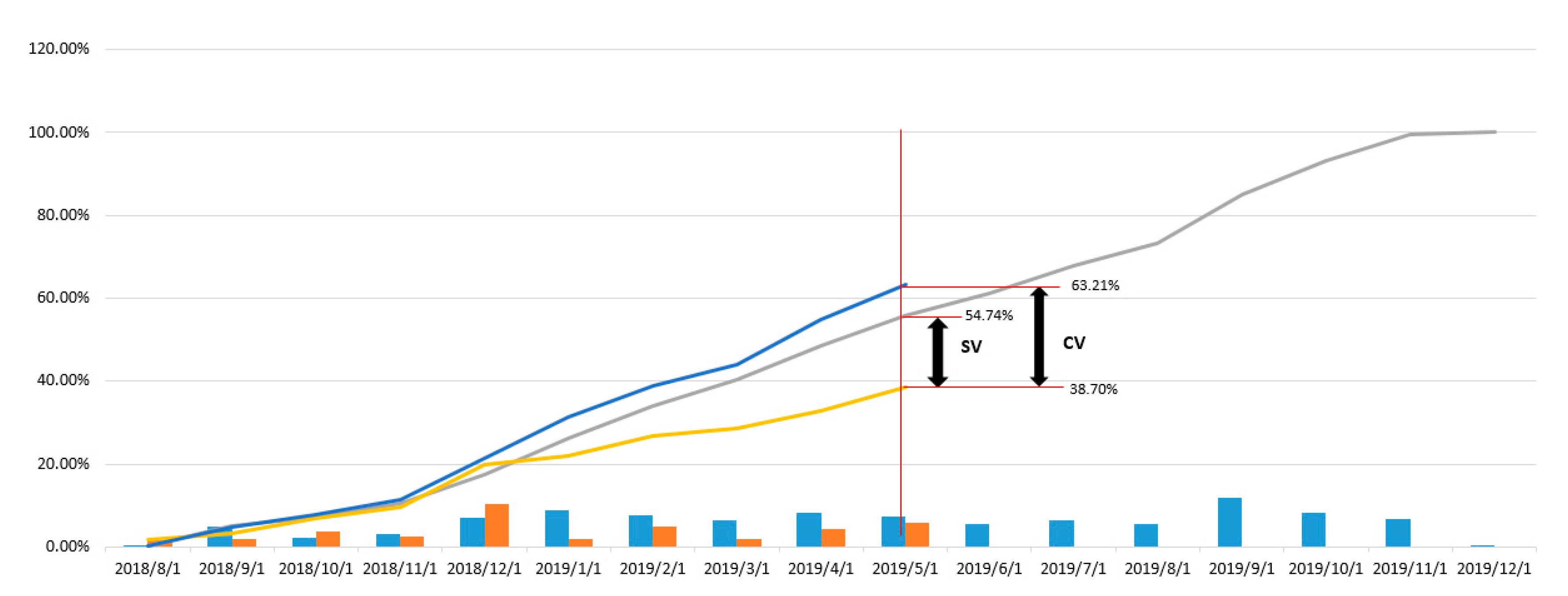
| 0.0152 | 0.727 | Traditional EVM |
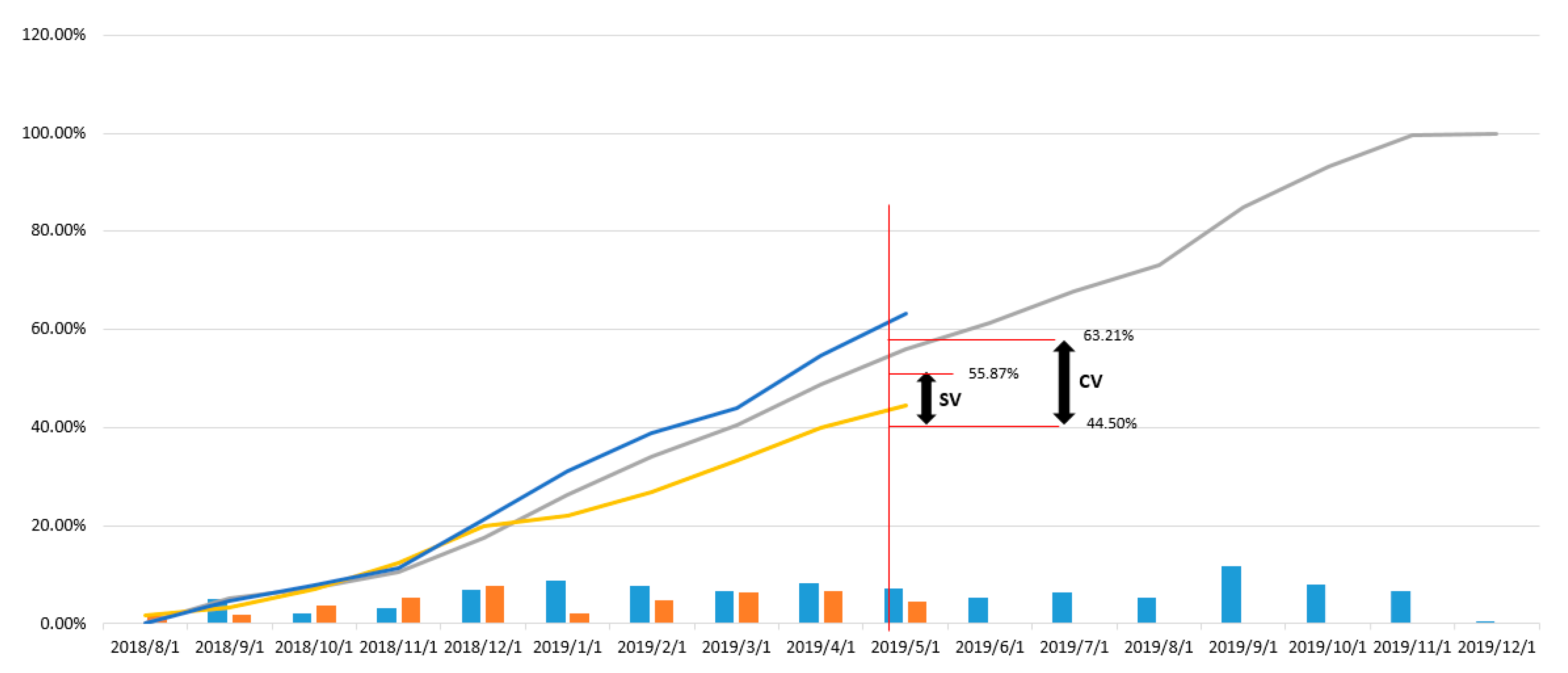
| 0.00206 | 0.896 | ANN |
| 0.012 | 0.864 | Multiple regression |
Publisher’s Note: MDPI stays neutral with regard to jurisdictional claims in published maps and institutional affiliations. |
© 2020 by the authors. Licensee MDPI, Basel, Switzerland. This article is an open access article distributed under the terms and conditions of the Creative Commons Attribution (CC BY) license (http://creativecommons.org/licenses/by/4.0/).
Share and Cite
Balali, A.; Valipour, A.; Antucheviciene, J.; Šaparauskas, J. Improving the Results of the Earned Value Management Technique Using Artificial Neural Networks in Construction Projects. Symmetry 2020, 12, 1745. https://doi.org/10.3390/sym12101745
Balali A, Valipour A, Antucheviciene J, Šaparauskas J. Improving the Results of the Earned Value Management Technique Using Artificial Neural Networks in Construction Projects. Symmetry. 2020; 12(10):1745. https://doi.org/10.3390/sym12101745
Chicago/Turabian StyleBalali, Amirhossein, Alireza Valipour, Jurgita Antucheviciene, and Jonas Šaparauskas. 2020. "Improving the Results of the Earned Value Management Technique Using Artificial Neural Networks in Construction Projects" Symmetry 12, no. 10: 1745. https://doi.org/10.3390/sym12101745
APA StyleBalali, A., Valipour, A., Antucheviciene, J., & Šaparauskas, J. (2020). Improving the Results of the Earned Value Management Technique Using Artificial Neural Networks in Construction Projects. Symmetry, 12(10), 1745. https://doi.org/10.3390/sym12101745


