Abstract
Over the past few years, the study of environmental sound classification (ESC) has become very popular due to the intricate nature of environmental sounds. This paper reports our study on employing various acoustic features aggregation and data enhancement approaches for the effective classification of environmental sounds. The proposed data augmentation techniques are mixtures of the reinforcement, aggregation, and combination of distinct acoustics features. These features are known as spectrogram image features (SIFs) and retrieved by different audio feature extraction techniques. All audio features used in this manuscript are categorized into two groups: one with general features and the other with Mel filter bank-based acoustic features. Two novel and innovative features based on the logarithmic scale of the Mel spectrogram (Mel), Log (Log-Mel) and Log (Log (Log-Mel)) denoted as L2M and L3M are introduced in this paper. In our study, three prevailing ESC benchmark datasets, ESC-10, ESC-50, and Urbansound8k (Us8k) are used. Most of the audio clips in these datasets are not fully acquired with sound and include silence parts. Therefore, silence trimming is implemented as one of the pre-processing techniques. The training is conducted by using the transfer learning model DenseNet-161, which is further fine-tuned with individual optimal learning rates based on the discriminative learning technique. The proposed methodologies attain state-of-the-art outcomes for all used ESC datasets, i.e., 99.22% for ESC-10, 98.52% for ESC-50, and 97.98% for Us8k. This work also considers real-time audio data to evaluate the performance and efficiency of the proposed techniques. The implemented approaches also have competitive results on real-time audio data.
1. Introduction
The evolution of cognitive science in the modern era involves the participation of audio recognition as an important factor. It has many applications in various fields of our daily life. Therefore, in smart cities, audio recognition can be used for security control systems [1], audio surveillance systems [2], disclosure of crime scenes by using audio and video [3], detection of urban noises in smart cities with the help of IoT-based solutions [4], traffic density movement and pollution control in the city [5], spotting the screams in gunshot scenes [6]. Other daily routine life applications include health care systems [7], audio recognition can be employed to monitor the health of distinct structures [8]. In forests, it can be employed to recognize distinct animals’ voices [9,10], to protect various endangered bird species in wildlife [11], or used in fire rescue operations [12]. Few of the recently developed usage of various sounds classification tasks in smart cities also involve the sound event detection in a parking garage [13] and for safety purposes in smart cities [14]. Due to its wide area of applications, auditory scene recognition has now become a hot research topic.
The audio classification and recognition research consists of three fundamental disciplines: sound event recognition, popularly known as ESC [15], automatic recognition of speech [16], and music category classification [17]. From the nature and structure of the domains discussed above, as stated in the literature, the classification of environmental sounds is a much more complex task due to the following reasons. First, the structure of ESC problems is different compared to music and speech signals [18]. Secondly, due to the involvement of both indoor and outdoor activities for ESC, the Signal to Noise Ratio (SNR) is very small because of a large distance between the microphone for the sound recorder and the audio generation source [19]. It may need to recognize confusing acoustic scenes from daily routine life, like, in restaurants, street traffic [20]. Sometimes, there is an overlap in audio events [21] and the existence of numerous sound sources [19]. All these exclusive syndrome structures made ESC tasks challenging enough compared with other audio sound recognition events.
The classification of environmental sounds generally involves the taxonomy of two basic major components: the utilization of the best acoustic features and the implementation of classifiers with better results. Normally, the audio features are extracted by separating the audio signal considered into frames with a hamming window. A set of features are extracted for each frame and used for training and testing [22]. There are numerous types of audio features. A few well-known features recently used for the classification of environmental sound events are discussed below:
- Frequency features: Few of the renowned acoustic features based on frequency are chroma features, mainly Chroma-based short time Fourier transform (Stft) [23], tonal centroid (known as Tonnetz) [24], spectral contrast (S-C) features [25].
- Mel filter bank-based features: These types of features are frequently used by researchers for the successful classification of environmental sounds. Mel frequency cepstral coefficient (MFCC) [26], Mel [27], and Log-Mel (LM) spectrogram [28] are popular Mel filters.
- Gammatone filter-related features: They are also known as dependent features. One of the popular gammatone filter-related features is the gammatone frequency cepstral coefficient (GFCC) based feature [29].
- Waveform-based features: The wavelet feature is one of the best examples of such a feature [30]. For recently published results see [31].
The aggregation of diverse features can have better results compared to single hand-crafted features. Our proposed methodology involves features based on the Mel filter bank, Mel, LM, and two new novel features extracted from these features known as L2M and L3M. In the experiment, all these features will be used as aggregated or accumulated features. After the selection of relevant features, the selection of suitable classifiers is the next challenging task to get state-of-the-art performances.
Various machine learning classifiers and techniques have been implemented to classify music and other acoustic events, such as random forest (RF) in [32], decision tree (DT) in [33], K-nearest neighbor (KNN) [34], and support vector machine (SVM) [35,36]. Recent researchers have reported the effectiveness of deep learning models over ordinary or machine learning classifiers. Many researchers used recurrent neural networks (RNNs) [28], convolutional neural networks (CNN), and transfer learning techniques [37,38,39] to get remarkable results for environmental sound detection tasks. CNN is also used in diagnosing faults in unmanned aerial vehicle (UAV) blades by using sounds in [40]. In this study, the transfer learning-based DenseNet-161 with cyclic learning rate is considered, and the resultant performance is extremely nice when considering those proposed data argumentation approaches for features.
In this study, new data transformation/augmentation techniques are implemented on ESC-10, ESC-50 [41] and Us8k [42] datasets. The proposed augmentation approaches are based on the SIF of the audio clips used. The main and important contributions of this experimental study are mentioned as follows:
- Two new and novel auditory feature extraction techniques, named L2M and L3M are introduced for SIF, as shown in Figure 1.
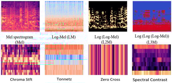 Figure 1. The spectrogram of various acoustic features used in this study.
 - The usage of trim silence, as an influential pre-processing technique is considered. The experimentation has been done with original, noise reduction, and trim silence approaches as a pre-processing technique, the best performance was achieved by trim silence with 40 dB as shown in Figure 2.
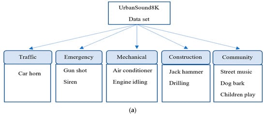
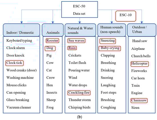 Figure 2. (a) The taxonomy of various classes in the Urbansound8k (Us8k) dataset. (b) The taxonomy of various classes related to ESC-10 and ESC-50 datasets.
 - A fine-tuning of the transfer learning model by using optimal learning rates in combination with discriminative learning is employed.
- Aggregation of various SIF in Section 3.5, which involves a total of seven aggregation schemes, including four double and three triple features accumulation approaches.
- The formulation of an exclusive new augmentation technique (named NA-1) for SIF based features is proposed. This approach is based on using a single image as a feature at a time.
- The advancement of the first data transformation capacity (NA-1) into another form (named as NA-2), which is a vertical combination of various accumulated features in the form of spectral images, is proposed.
- True testing is conducted by generating real-time audio data from YouTube for better investigation and analysis of our proposed methodologies.
- The conversion of audio to spectrogram and implementing various augmentation techniques on those SIF is very rarely applied, and according to the best of our knowledge, the data enhancement of spectrogram images for environmental sound classification task was not previously applied.
The structure of the rest of the manuscript is organized as follows: Section 2 provides a literature review related to the environmental sound classification problem. Section 3 demonstrates the scheduled procedure or methodology to carry out the experiments. This section also exhibits the in-depth details of the datasets used. Besides, the necessary software and hardware requirements to execute the experiments are also given in this section. Section 4 displays the final results and discussions. Finally, the last section includes conclusive remarks to wind up this work.
2. Related Works
The popularity of the classification of sound event recognition (SER) taken from the environment is increasing very rapidly nowadays. The numerous and distinct datasets have been available related to the ESC domain. This study involves three popular datasets related to ESC tasks: ESC-10, ESC-50, and Us8k. The baseline paper, which generated ESC-10 and ESC-50, first involves distinct machine learning and ensemble models like K-NN, SVM, and RF, which have been implemented on ESC datasets. The best accuracy is achieved by ensemble technique RF in [41]. In another study, the author, Silva et al. proposed various classical machine learning techniques for recognizing urban sounds. The K-NN, naïve Bayes, SVM, DT and artificial neural network (ANN) were tested on ESC datasets, and the best performance was achieved by K-NN in [43]. In later experimental work [44], CNN was successfully tested on ESC datasets and beat the baseline models with a marginal difference. In [45], Zhou et al. proposed a new convolutional network on Us8k and gained an accuracy of 86%. The author, Demir et al. [46] proposed a new deep convolutional neural network (DCNN) model on Us8k and got an average accuracy of 86.7%. In [47], Chen et al. suggested a new method of dilated convolution on Us8k and achieved an accuracy of 78%. Hertel et al. trained and tested DCNN and CNN on ESC-10 and gained an accuracy of 77.1% and 89.9%, respectively in [48]. Pillos et al. [49] investigated the environmental sound recognition system for the Android operating system (AOS) on ESC-10. Ahmad et al. [50] gained an accuracy of 87.25% on ESC-10 by implementing an optimum allocation sampling technique. Medhat et al. suggested masked CNN on used ESC datasets to get high accuracy in [51]. Singh et al. narrated a method of using a single value decomposition method in one dimensional CNN for ESC-50 and attained remarkable results, as explained in [52]. Abdoli et al. [53] has also implied 1-D CNN for Us8k with an accuracy of 89%. Li et al. recommended a multi-stream network with a temporal attention network in [54], which was computed through a consecutive energy change, with remarkable accuracy of 94.2% and 84.0% on ESC-10 and ESC-50.
The involvement of the extracted features with a machine and deep learning models also played an essential part in the classification of ESC problems. In this work [36], a combination of different features have been implemented by using SVM. The author narrates the new approach by aggregating the global and local features on Us8k in [55]. Chong et al. proposed multi-channel CNN with multiple feature fusion techniques in [56], and the highest accuracy achieved was 73.1% for ESC-50, 87.6% for ESC-10, and 75.1% for Us8k. Ming et al. [57] examined the psychoacoustic features implemented on four different environment sound recognition datasets, including Us8k and ESC-50 by using a neural network (NN). The average achieved accuracy was 85.69% and 86.99%, respectively. Sharma et al. have proposed stacking the channels with multiple features by using variable DCNN groups of distinct layers. The author stated remarkable results on all used ESC datasets in [58] after adding the strong augmentation. In this reference [59], transfer learning methodology is also used and attains astonishing results on all used ESC datasets.
The research works mentioned above provided many positive observations and understanding of the very heterogeneous and complex datasets used in this study. In this manuscript, we addressed two unique and new features with their involvement in exclusive and offbeat new augmentation approaches. Later these data enhancement techniques were tested on real-time audio datasets, similar to original audio recordings, collected from YouTube. In the adjacent section, the details have been discussed with proposed methodologies and related materials in this paper.
3. Methodology
This section includes the detailed description of used datasets with experimental setup and collection of the real-time audio recordings in resemblance with original datasets. These segments also considered the description of used acoustics features and their accumulation. The proposed data augmentation approaches have also been implemented in this experimental study. The use of transfer learning with cyclic learning technique with optimal learning rates for environmental sound classification is another contribution. The last sub-section includes the discussion about the popular metrics to evaluate the performance of models.
3.1. Spectrogram Based Acoustics Features Extraction Techniques
3.1.1. Log-Mel (LM) and Mel-spectrogram (Mel)-based Features
The Mel spectrogram is the portrayal of the sound in the form of time and frequency. It is fragmented into several points that equally distribute frequencies and times on a scale of Mel frequency. The relationship of the Mel frequency scale and its inverse has been defined as follows:
where Mel belongs to Mel-based frequency and f is represented as a normal frequency. The Log-Mel has been calculated by taking the log on the Mel-spectrogram. In this study, the power spectrogram of the LM has been utilized, which is generated by Equation (4) elaborately discussed in the next sub-section.
3.1.2. New Mel Filter Bank-Based Proposed Log2Mel (L2M) and Log3Mel (L3M) SIF Features
The conversion of the logarithmic scale Mel spectrogram features into L2M and L3M includes the transformation of power spectrograms, related to amplitude square, into a decibel unit (dB). The scaling process needs to be done numerically in a very reliable and stable way. The following equation represents the scaling:
where S is the input power, which is in the form of an array and ref represents the reference value. The Librosa library has been used for generating L2M and L3M acoustic features in terms of a spectrogram. The above Equation (3).
Steps to find L2M and L3M SIF:
- Consider an audio waveform.
- Convert the audio recordings into Mel-spectrogram-based log-power spectrograms.
- The selection of reference ‘ref’ involves two possibilities. (i) The computation of decibels (dB) is comparable to peak power for reference value. (ii) Evaluate decibels (dB) relative to median power, for the consideration of reference value. We selected the decibels related to the peak power, case (i).
- After the selection of reference value ‘ref’, it returns the input power ‘S’ to decibel (dB) and is represented in Equation (4), which gives the LM SIF feature:
- The L2M feature is demonstrated as follows:
- The representation of L3M was conceived as below:where S denotes the input power, ref is the reference value, are the power spectrogram for LM, L2M, and L3M respectively. Both new features images have been exhibited in Figure 1. Although the individual performance of these L2M and L3M audio feature extraction techniques was less satisfactory in comparison with other Mel filter-based features (LM & Mel), they outperform and show competitive performance in comparison with few famous acoustics features ((S-C), Tonnetz, zero cross rate (Z-C) and chroma Stft (C-S)). These two features also play a very crucial role in our new augmentation methods to achieve a state-of-the-art result.
3.1.3. General Audio Features
(1) Zero Cross Rate (Z-C): This feature is known as the frequency content of the sound signal. It is the measure of the total number of times, the amplitude of the audio signal crosses the zero value in a given interval of time and frame. It has numerous applications specifically used in the classification of distinct musical instruments [60] and segregation between unvoiced and voiced signals [61]. According to the definition, Z-C is defined as follows:
where:
where wd is the window function and N is the total number of samples in Equation (9):
(2) Chroma features (C-S): Chroma features are extensively used for the analysis of the music signals [62] and various recognition projects, including the environmental sound classification task [31]. The description of the chroma feature includes the division of the audio signal pitch into two components in [63]. One is chroma, and the other is tone height. After the estimation of equal-tempered scale values, the 12 chroma attributes can be set as {C, C#, D, D#, E, E#, G, G#, A, A#, B}, which are famously known as western music notation. This 12-dimensional values vector is denoted as z = (z1, z2, …… z12)T. These terms z1 coincide with chroma C, z2 corresponds to chroma C#, respectively up to the last element, z12 corresponds to B.
The harmonic content of the short time window of the sound signal has been represented by the chroma features. The magnitude spectrum assists the extraction of these feature vector by the following well-known methods. Constant-Q transform (CQT), short time fourier transform (STFT), chroma energy normalized statistics (CENS), etc. This study implemented STFT; the signal has been converted into smaller windows and then the sequence of Fourier transform was applied to these signals. STFT contributes to the information of frequency components related to the signal, which changes over time. The STFT pair has been defined as follows:
where x[k] is the signal and y[k] is the window function and m is discrete and n is continuous. L denotes the length of a window function. X [m, n] represents the nth fourier coefficient for the mth time frame.
(3) Tonal centroids (Tonnetz): Tonal Centroid is a depiction of a pitch. It is also recognized as a harmonic network, Harte et al. [24]. Let Tnx is a Tonnetz vector with a time frame of x. This Tonal centroid (Tnx) vector is an outcome of the product of the transformation matrix Tf and chroma vector denoted by Chx. To avoid numerical uncertainty and establish the presence of the Tonnetz vector in a six-dimensional space, the above result is divided by the L1 norm of the chroma vector. The Tonnetz vector is defined as follows:
where d is the six-dimensional evaluation index, and m is the class index of chroma vector pitch.
(4) Spectral contrast (S-C): The acoustic feature, which speaks for the spectral contrast, represents the fortitude of spectral valleys, peaks, and their differences, as demonstrated in [25]. The process involves slicing audio waveforms into 200 ms windows with overlapping of 100 ms. The spectral components have been achieved by performing the fast fourier transform (FFT) on each frame. In the next step, these components are segregated into six octave-scale-based sub-bands, one by one. At last, the strength of spectral valleys and peaks has been estimated by the small neighborhood, average value. The detailed expressions have been demonstrated as follows:
Let {yx,1, yx,2, ……… yx,n } represents the FFT vector of xth sub-band, where yx,1 > yx,2 > … >yx,n. The firmness and stability of the spectral valleys and spectral peaks have been predicted as follows:
The difference of the spectral peak and spectral valley in spectral contrast (S-C) is defined as follows:
whereas alpha ( is a parameter of a small neighborhood with a value of [0.02, 0.2], n is equal to the total in the xth sub-band with x belongs to {1, 6}.
3.2. Experimental Datasets and Setup Description
This experimental analysis involves two major environmental sound classification datasets: the ESC-50 [41] and the Us8k [42]. These datasets have been comprised of non-overlapping audio clips, recorded in various environments and distinct noise levels. The ESC-50 dataset includes 2000 audio clips with 5 s average length of each file. The ESC-50 dataset was sampled at 44,100 Hz and uniformly distributed 50 classes into five folds, respectively. Each class consists of 40 audio files each. The taxonomy of sound classes in ESC-50 involves five main groups. These are natural soundscapes with water, human sounds (non-speech), animals, indoor domestic sounds and outdoor urban sounds. The ESC-50 dataset further divides into another subset dataset known as ESC-10. This dataset contains 400 audio files with a systematic distribution of 10 classes into five folds. These balanced classes are (dog bark, sea waves, rain, baby crying, person sneezing, clock tick, chain saw, helicopter, fire crackling, rooster).
The Urbansound8k data set contains 8732 labeled audio files with a length of 4 s for each clip. This dataset is widely used by most researchers to evaluate the performance of their models on ESC tasks. This dataset consists of 10 non-uniform and imbalanced classes: car horn, air conditioner, children playing, dog bark, drilling, jackhammer, siren, gunshot, engine idling, street music. These classes have been assigned to 10 folds irregularly. The estimated playing time of all audio clips was 9.7. The concise taxonomy of all the used datasets has been illustrated in Figure 2.
The real-time audio data has also been collected from YouTube to test the performance of our proposed methodologies. Only one-fold gathered, related to the classes of each used dataset. For ESC-10 and ESC-50, both datasets have a uniform distribution of audio classes in folds. The real data of 80 audio clips associated with ESC-10 and 400 real-time audio recordings linked to ESC-50 have been compiled. The allocation of data for Us8k was imbalanced with the non-uniform distribution of classes in each fold. A total of 500 audible clips has been allocated relevant to the Us8k dataset. These real-time audio recordings from YouTube have only been used to analyze and test the performance of proposed methodologies and had not been used for training purposes. The details about the real-time collected data have been discussed in Table 1.

Table 1.
Description of real-time audio clips.
Hardware and Software Specifications of the System
The hardware specification of the system used in this experiment is Intel(R) Core™ i9-7900X CPU with a clock speed of 3.30 GHz and 64 GB RAM. The hard drive used was 1 TB HDD + 1 TB SSD. The graphical processing unit (GPU) power of the system is associated with Nvidia, GeForce, 2 X GTX 1080, 11 GB VRAM, each with a total memory capacity of 22 GB.
The various packages and API libraries have been used in the experiment to implement the proposed architecture with the help of the transfer learning model. The operating system (OS) used in this study was Ubuntu 18.04.3 LTS, 64 bit. The famous Python-based artificial intelligence frameworks used in the experiments are as follows:
- Librosa: It is a Python package normally used for the analysis of audio and music signal processing [64]. Its various functions involve feature extraction, decomposition of spectrograms, filters, temporal segmentation of spectrograms, and much more. In this study, this package was used to extract spectrogram images features like Mel, LM, C-S, S-C, and other features extraction techniques-based images from audio files or clips.
- Fast.ai: It is an artificial intelligence framework that makes it easier for everyone to use deep learning effectively [65]. The main focus of this library is to advance the capacity and techniques which help the model to train quickly and effectively with limited support and resources. The implementation of transfer learning models with the help of pre-trained weights and the concepts of discriminative learning and fine-tuning have been done in this package.
- Audacity: It is an open-source digital audio recorder and editor. It is freely available with very user-friendly properties for all types of operating systems like Windows, Linux, and macOS. The YouTube-based audio dataset for the testing and evaluation of our proposed models have been recorded and edited through this package [66].
3.3. Preprocessing Technique
Trailing and trimming the silence portion from an audio clip or signal is one of the common augmentation techniques. In this manuscript, this transformation technique is used as a pre-processing approach because the audio datasets used in this study involve sound clips, which are prolonged from 4 to 5 s, individually. Many classes in ESC-10 and ESC-50 include the audio files which contribute only 30% to 40% time of the audio clip as an original sound, with a remaining portion as a silence. Such type of audio data dramatically decreased the classification accuracy of the model. In this experiment, the vacant or silence portion of the audio clips have been trimmed by using the trim silence function in [64] Librosa package.
One of the common problems while using trim silence as a pre-processing technique on the whole audio data sets was finding the exact threshold value in decibels (dB) below the reference point to recognize as a silence. The inaccurate selection of the threshold value can result in a loss of critical information, present in our audio data. In this experimental study, several repetitive tests have been performed to find the most suitable threshold value for used environmental sound classification datasets. The 10 dB, 20 dB, 40 dB, 50 dB, and 80 dB were the breakeven points, which have been investigated on each data set separately. The 40 dB threshold value has been settled as the most effective silence trimming value for the used datasets. Figure 3. shows the example of a signal.
Figure 3.
The dog class ESC-10 dataset, (a) original, (b) 10 dB, (c) 20 dB, (d) 40 dB, (e) 50 dB, (f) 80 dB trimming. The 40 dB trimming as a best trimming silence option for ESC datasets.
3.4. Aggregation of Different Acoustic Features
The accumulation of various audio features into one spectrogram is one of the new and exclusive approaches to get better results. The use of the aggregation of such acoustic features assists the model to overcome the factor of lower eigenvectors values. The involvement of these values does not allow CNN based models to adequately classify the environmental sounds. Therefore, the combination of distinct audio features leads to successful classification.
This study also proposed the accumulation scheme of the double and triple features. Firstly, the two new features have been integrated horizontally to make a single feature set called NC. For double features aggregation, the NC feature set will be combined with another single spectrogram-based feature in such a way that dimensions of both features will be equal in terms of width X height. In the same context, for triple aggregation, the NC, will be incorporated with the vertical coalition of two separate audio features. The image representation of used aggregated auditory features is shown in Figure 4. Let FtM, FtLM, FtL2M, FtL3M, FtSC, FtCS, FtNC represent features in the form of spectrogram images related to Mel, LM, L2M, L3M, S-C, C-S, and NC which is the horizontal combination of two new acoustic features L2M and L3M. Let ⊕ denote the vertical linear superposition operation and ⊕′ represent the horizontal superposition, then FtNC = FtL2M ⊕′ FtL3M. The seven features aggregation strategies, including four double features and three triple features accumulation, are described as follows.
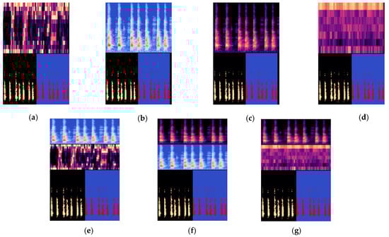
Figure 4.
The image illustration of seven aggregated auditory features, (a) CS-NC, (b) LM-NC, (c) M-NC, (d) SC-NC, (e) LM-CS-NC, (f) M-LM-NC, (g) M-SC-NC.
3.4.1. Double Aggregated Features
- (1)
- M-NC: The vertical combination of Mel spectrogram and NC, represented as:FtM-NC = FtM ⊕ FtNC.
- (2)
- LM-NC: The vertical combination of LM and NC, expressed as:FtLM-NC = FtLM ⊕ FtNC.
- (3)
- SC-NC: The vertical combination of S-C and NC, represented as:FtSC-NC = FtSC ⊕ FtNC.
- (4)
- CS-NC: The vertical aggregation of C-S and NC, expressed as:FtCS-NC = FtCS ⊕ FtNC.
3.4.2. Triple Aggregated Features
- (1)
- M-SC-NC: The vertical combination of Mel, S-C, and NC expressed as:FtM-SC-NC = FtM ⊕ FtSC ⊕ FtNC.
- (2)
- LM-CS-NC: The vertical combination of the LM, C-S, and NC expressed as:FtLM-CS-NC = FtLM ⊕ FtCS ⊕ FtNC.
- (3)
- M-LM-NC: The vertical combination of Mel, LM, and NC expressed asFtM-LM-NC = FtM ⊕ FtLM ⊕ FtNC.
3.5. Transfer Learning Model (DenseNet-161) with Fine-tuning (Strategy-2) and without Fine-Tuning (Strategy-1)
The term transfer learning is nowadays very common in solving various deep learning-related problems. This terminology means using the knowledge of other pre-trained models trained on a large number of images dataset for your custom requirement or purpose. This technique is usually used by researchers to avoid training their models from scratch. Many also preferred this approach because they do not need to define the architecture of their used CNN model. The use of transfer learning models becomes very helpful when the targeted data is small. Transfer learning is a procedure of overcoming the detached learning paradigm and employing the information and expertise obtained for some particular task to solve other associated problems. For example, the knowledge of transfer learning has been used for the classification of medical images and acoustic sound events recognition from a real-life scene in [67,68].
3.5.1. ImageNet
In this experimental study, a concept of using a pre-trained model with fine-tuning and without fine-tuning. This transfer learning-based model trained on the very bulky data set of images, known as ImageNet. It is a collection of a large number of photographs randomly collected by a human. These images are used by different researchers and academics experts to develop state-of-the-art computer vision algorithms. It includes more than 14 million images with 21,841 categories. The number of images with scale-invariant feature transform (SIFT) features are 1.2 million images used for the training and about 0.1 million for the testing and 0.05 million for the validation purpose. This SIFT feature-based dataset consists of 1000 distinct categories or classes in [69].
3.5.2. DenseNet-161
This transfer learning model consists of the convolutional networks which are more accurate, deeper, and effective for training. It contains more concise connections between the input and output layers. Each layer is connected in a feed-forward fashion to all the other layers. We don’t need to train this model from scratch. This model is very strong in feature propagation and manipulation. It also extensively reduces the total number of parameters. In this research, we implemented DenseNet-161 [70] model on our aggregated and augmented spectrogram images.
The architecture of DenseNet-161 includes the input layer, dense layers, transition layers, and fully connected layer concatenated by a global average pooling layer. The convolutional and max-pooling function used in the model involves the various number of filters to pursue the process of feature extraction from the images. These filters are in the form of a symmetrical window with various kernel sizes. These symmetric windows-based filters play a crucial role in convolution and max-pooling followed by the input layer, dense, and transition layers. The transfer learning-based structural model used in this study contains a different number of kernels. The division of these symmetric filters for each layer of the model is as follows: Input layer (convolutional; total 96 filters/7 × 7 sizes), (max-pooling; total 96 filters/2 × 2 sizes). Each transition layer is comprised of a single filter with 1 × 1 and 2 × 2 conv sized. The dense layers are distributed into 4 blocks. The first block contains 6, the second block includes 12, the third block holds 36, and the fourth block comprehends 24 filters with a 1 × 1 conv and 3 × 3 conv sized. The fully connected layers of the model remained the same but the output layer has been modified to the total number of categories used in the experimental data.
3.5.3. Explanation of Proposed Methodologies
The division of the pre-trained transfer learning models normally exists in two parts. The first one is the convolutional base section, which includes the set of convolutional and pooling layers. The basic goal of this partition of the model is to determine the features of the images. The second part is comprised of the fully interrelated layers, popularly known as the classifier. The main task of this part is to categorize the images by using the detected features, identified by the convolutional base. As described in [71], the first portion of the convolutional base is further split into two domains of layers. The early or initial layers of the convolutional base are set to find out the general features in the form of straight lines, curves, edges, etc. The last or final layers aim to capture the specific and important features like shape, etc. The model must train well, especially at the point of the transition from the general to the special distinctive features part in the network.
While using the transfer learning models for the custom-based datasets, a few approaches are very useful. As the classifier part with the fully connected layers is focused to predict the actual classes of the images used in the datasets. Therefore, the removal of the fully connected layers from the models and add up a classifier with a new set of fully associated layers to meet the requirement of new classes in the custom datasets. In this experimental study, we want to implement the transfer learning model DenseNet-161 with ImageNet weights on our spectrogram images datasets for the classification of environmental sounds. Our accustomed datasets were very small and also different from the original ImageNet dataset on which these transfer learning networks were trained. Hence, the chances of overfitting were extremely high, and it was also very difficult to find the exact balance between the layers. Consequently, it is very hard to achieve state-of-the-art performance on the environmental sounds distinct spectrogram images dataset by using ImageNet weights. Thus, this exploratory research implemented the combination of different methodologies to get up to the mark results. The applied approach consists of the concept of fine-tuning the transfer learning model. The earlier layers part from the convolutional base, which is independent of the targeted problem, is frozen so its weight should not change during the training and train the remaining layers (final layers of the convolutional base and fully connected layers) to find the optimal learning rate for each used dataset. In the next step, unfreeze all the frozen layers and re-train the network by using a discriminative/cyclic learning technique that follows the range of optimal learning rates. This methodology achieves remarkable performance in just seven epochs. Figure 5a shows the ordinary method of transfer learning strategy-1, and Figure 5b, strategy-2, discussed the details of the implemented approach in terms of block diagram (fine-tuned).
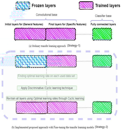
Figure 5.
Block diagram of fine-tuned pre-trained weights through Cyclic learning by using optimal learning rates. (a) Strategy-1, (b) Strategy-2.
3.5.4. Discriminative/Cyclic Learning
The concept of using cyclic or discriminative learning is very important for the better performance of the model. It is very complex and quite tricky to train a model on a single learning rate. If the learning rate became very small, then it would take a very long-time span to reach the global minima point. On the contrary, the larger the learning rate, the higher the risk of getting the maximum loss function value. Therefore, the idea of discriminative learning proposed the distribution of the layers of the model into three batches. The first batch includes the initial convolutional learning layers with a lower learning rate, so the model would be able to learn the small details, for example, straight line and edges, etc. in depth. The second batch involves the remaining convolutional layers with a slightly larger learning rate. The function of these layers is to determine the crafty and complex structures or patterns, for instance, squares, circles, etc. The final and last batch of dense layers is trained on the maximum optimal learning rate. Although there were numerous methods related to the learning rate, the most popular methods are adaptive learning [72,73], and cyclic learning [74]. Figure 6. indicates the cyclic learning rate in the block diagram.
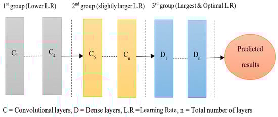
Figure 6.
Block diagram of the cyclic/discriminative learning rate.
3.5.5. Determination of Optimal Learning Rates for Used Datasets
The determination of the superlative learning rate for our model on each dataset individually involves the phenomena of freezing and unfreezing layers. It is very convenient to find the optimal learning rates with the help of the Fast.ai [65] package. The procedure includes the training of the model while freezing the initial convolutional layers. Repeat this process, but this time, unfreeze all layers. Figure 7. illustrates the optimal cyclic learning rate for ESC-10, ESC-50, and Us8k datasets.
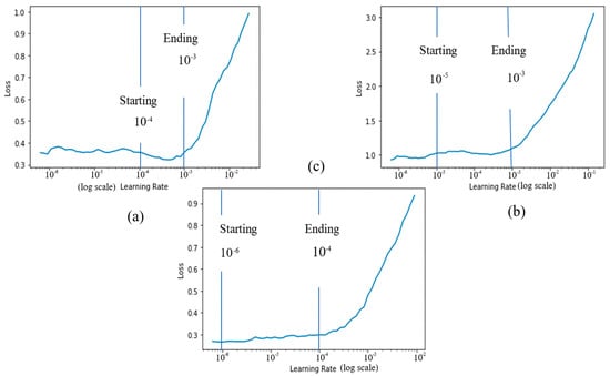
Figure 7.
The optimal and discriminative learning rates of each used dataset. (a) ESC-10 (10−4, 10−3), (b) ESC-50 (10−5, 10−3), (c) Us8k (10−6, 10−4).
3.6. Data Enhancement Approaches
The convolutional neural network can classify various classes of images. It also illustrates extraordinary performance on the classification of different sounds based on their spectral images. It can distinguish the noise with original sounds that are masked in time or frequency. The major drawback of CNN is the extensive amount of data to train and huge computational power required. The deficiency of a large amount of data for training purposes can be solved by using appropriate data augmentation techniques. In this process, the synthetic data has been assembled with original data introduced to overwhelm the risk of overfitting. This technique is known as data transformation/augmentation [75]. The augmentation for audio data has become very popular these days to increase the certainty of the model. There are numerous ways to perform this work i.e., [76], but there is no published appropriate study that can enhance audio data available in the form of spectral images. The normal image augmentation approaches used for the classification of images [77,78] are not well suitable for this assignment. The astonishing change in the angle, height, brightness, width, etc. of spectrogram images dramatically decreases the accuracy of the model, although it can increase the number of data. Therefore, there is a dire need to determine a method to dilate spectral images data, which should have the ability to resolve overfitting issues and improve the accuracy of the model. This study proposed two new data augmentation schemes for the spectrogram images named NA-1 and NA-2, which have been demonstrated below. The proposed augmentation schemes are implemented only on the best-used new acoustic features and Mel filter-based features.
3.6.1. The First New Augmentation Technique for SIF (NA-1)
In this augmentation approach, the SIF data has been boosted in a unique way to reduce the risk of overfitting, as shown in Figure 8. After using trim silence as a pre-processing, the audio augmentation has been done twice on the whole trimmed data. Firstly, audio augmentation with white noise by a coefficient of 0.005 and later, the time-delay has been included by a factor of 0.80 in the audio sound data. This audio transformation has been done on the Librosa package [64].
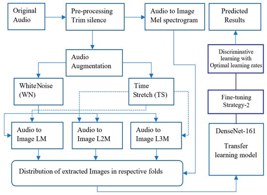
Figure 8.
The framework of the 1st New augmentation approach for spectrogram images (NA-1).
3.6.2. The Second New Transformation Approach for SIF (NA-2)
This second spectral image data enhancement approach, NA-2, is the exaggerated state of the NA-1. The only difference is that NA-2 used the aggregation of various audio features to enlarge the datasets despite utilizing a single feature image at a time. The advancement in the data has been done based on the combination of two features at once.
The accumulation scheme of various audio features has been categorized based on priority. The augmented data from New Augmentation-2 (NA-2) has been generated by the aggregation of one feature with other features in a linear way while using two features at a time. All the aggregated eigenvectors belong to two-dimensional feature vectors. The highest precedence has been granted to the original audio-based images of the Mel spectrogram. The second and third priority has been given to each time stretch log-Mel (TSLM) and white noise log-Mel (WNLM). Similarly, the preference has been provided to augmented features associated with L2M, and, in the end, it came to the features affiliated with L3M. Figure 9 exhibits the total features of aggregation possibilities without considering any repetition. The terms Fu and Fnu represent the feature used and feature not used. The linear superposition operation has been indicated ⊕. Table 2 shows the combinational schemes of the features used and not used in our experimental work. Figure 10 shows the proposed framework for the NA-2 augmentation approach for spectrogram images.
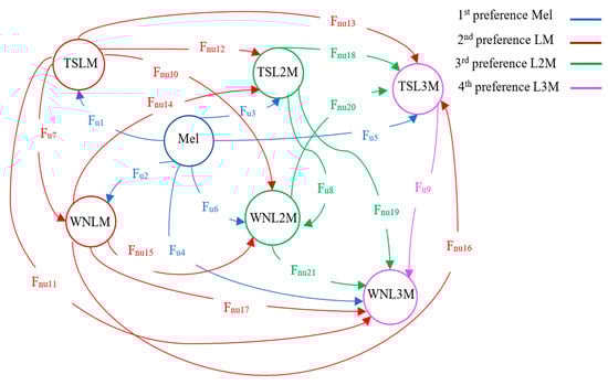
Figure 9.
The priorities and possibilities of various features accumulation schemes for the NA-2 augmentation.
Table 2.
The combinational strategies of consolidated features, utilized in the (NA-2) approach.
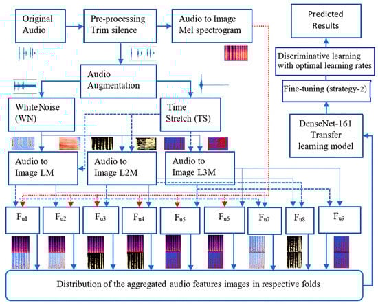
Figure 10.
The framework of the 2nd New augmentation approach for spectrogram images (NA-2).
3.7. Performance Evaluation Metrics
The execution of the transfer learning model on distinct acoustics features with aggregation and augmentation techniques have been tested by using confusion matrix-based performance assessment metrics. Such type of metrics has been widely used in various sound classification tasks like in [46]. Most of the studies evaluate the performance based on accuracy, error rate, precision, recall, and F1-score. This study used 10 important parameters to assess the execution of the model on different augmentation and features aggregation approaches involving distinct acoustic features. These metrics involve few crucial terminologies used in the confusion matrix. These are known as true positive (TP), false positive (FP), true negative (TN), and false negative (FN). Some other terms used for the evaluation of results in this study are true positive rate (TPR), false negative rate (FNR), and positive predictive value (PPV). In Equation (25), Y is the number of codes, and mij, xij, wij are the elements in expected, observed, and weight matrices. Based on these factors, the implemented evaluation metrics discussed in [79,80] are described as follows:
4. Experimental Results and Analysis
The state-of-the-art results have been reported in this manuscript on the ESC standard and baseline datasets, i.e., ESC-10, ESC-50, and Us8k by using suggested methodologies and models. The testing and training part on these datasets has been done according to the K-fold cross-validation [41,44]. The recommended K-fold setting by the baseline model papers is as follows. For the Us8k dataset, k = 10 and for ESC-10/ESC-50, k = 5. The DenseNet-161 model has been trained for 7 epochs. The acoustic features used in this experimental study have been categorized into two groups with four features in each group. One group of features includes general audio features like S-C, Z-C, C-S, and Tonnetz. The other group includes attributes based on the Mel filter bank, which also involves four acoustic features Mel, LM, and two new novel features, L2M and L3M. The experimental results in this study comprise seven sub-sections. The first part consists of the results with simple transfer learning (Strategy-1). The second portion includes the transfer learning with freezing/unfreezing layers (Strategy-2) with optimal learning rates based on discriminative learning. The third section comprehends the results with various features aggregation schemes with (Strategy-2). The fourth portion involves the performance evaluation of new augmentation approaches on all used data sets. The second-last part contains the comparison of features aggregation and new data enhancement techniques on real-time audio data. The final part comprises the comparison of proposed methodologies with previously published studies and baseline models.
4.1. Evaluation of the Results of all Features Extraction Techniques Through (Strategy-1)
The assessment of the DenseNet-161 transfer learning model has been carried out on various feature extraction techniques like Mel, LM, L2M, L3M, S-C, C-S, Z-C, and Tonnetz. The genuine and prescribed method of K-fold cross-validation has been conducted on all used datasets. In the next step of the experiment, these spectral images have been used to train the weights of DenseNet-161. Initially, the randomly selected learning rate of 10-4 has been used on all datasets. The performance of the model has been tested on a single fold at a time while the remaining folds are used for training purposes. Figure 11a elaborates on the performance of pre-trained weights for different acoustic features on the ESC-10 dataset. As shown in the figure, the new L3M audio feature attains the best accuracy in fold1 and fold4, and L2M achieved the highest results in fold5. The least accuracy was obtained by the Z-C feature in all folds. The overall highest average accuracy was 82.50% gained by the L3M feature. Figure 11b,c illustrate the accuracy comparison of all used audio features on the ESC-50 and Us8k datasets. The Mel feature obtained the best result on each dataset. Although the two new features, L2M, L3M, show less accuracy in Mel filter-based features, the group attained a huge margin in terms of accuracy compared with group-2 general audio features. The remaining efficiency parameters with average training time have been presented in Table 3.
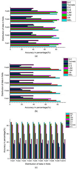
Figure 11.
(a) Fold wise classification accuracies of (Strategy-1) implemented on various audio features on the ESC-10 dataset. (b) Fold wise classification accuracies of (Strategy-1) implemented on various audio features on the ESC-50 dataset. (c) Fold wise classification accuracies of (Strategy-1) implemented on various audio features on the Us8k dataset.
Table 3.
The performance evaluation metrics of all extracted sound features with (Strategy-1).
4.2. Evaluation of the Results of all Features Extraction Techniques Through (Strategy-2)
In this section, the results of the exclusive proposed method of freezing/unfreezing the layers and re-trained the model with optimal learning rates with a concept of discriminative learning were used. All the ESC datasets undergo this approach with a perception of cyclic learning procedure through perfect learning rates for each dataset. The results shown in Table 4 reveal a major improvement in the accuracy and all other performance evaluation metrics. Only the training time increases due to the training with freezing layers to find the optimal learning rate and then again, re-training after unfreezing the layers. In cyclic learning, the initial suggested learning rate is lower and gradually increases to assist the model in getting closer to minima. Figure 12a–c illustrate the accuracy of the model with implied auditory features along respective folds. Table 4 elaborates that this approach efficiently increases the accuracy of the model on each auditory feature. The highest and the lowest gain in the accuracy of used acoustic features between this approach (Strategy-2) and previously discussed in Table 3 simple transfer learning methodology by using Strategy-1 has been discussed as follows: For the Us8k dataset, the feature S-C achieved the top accuracy gain of 28.93% and lowest accuracy gain attained by Mel, which was 7.77%. While considering the ESC-50 dataset, again, the maximal gain of 7.10% in the accuracy obtained by S-C and the least gain of 2.45% was achieved by Z-C. For the ESC-10 dataset, once again, the largest improvement in the accuracy was in the comparison of Table 4 with Table 3, earned by the S-C feature, which was 29.25% and undermost progress of 8.5% increase was attained by Mel. The results show marvelous improvement in the accuracy of all auditory features, but this methodology leads to one drawback related to the training time constraints, which also increased up to three times, related to the original training time of the model. Table 4 presented the detailed evaluation metrics for this approach.
Table 4.
The performance evaluation metrics for all used auditory features on the DenseNet-161 model (Strategy-2).
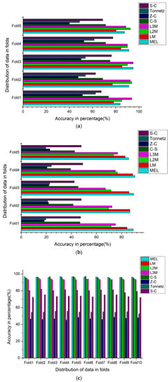
Figure 12.
(a) Fold wise classification accuracies of the DenseNet-161 model implemented on various acoustic features by using (Strategy-2) on the ESC-10 dataset. (b) Fold wise classification accuracies of the DenseNet-161 model implemented on various acoustic features by using (Strategy-2) on the ESC-50 dataset. (c) Fold wise classification accuracies of the DenseNet-161 model by using (Strategy-2) on the Us8k dataset.
4.3. Performance Evaluation of All Features Aggregation Techniques by Using (Strategy-2)
In this part of the manuscript, the top-performing auditory features from previous results were selected and further accumulated with each other in various settings. The horizontal combination of two new acoustic features L2M, L3M, were aggregated and named this featured pair as NC. In double features accumulation, this NC feature set combined vertically with another feature in such a way that the dimension of the overall feature set would be equal to 105 × 218. Similarly, for the triple aggregated features, the dimensions of the accumulated features would be identical. The only difference was that this agglomeration consists of the vertical combination of two different audio features with NC. This study investigates all the features aggregation techniques with identical dimensions.
The fivefold cross-validation for the ESC-10 and ESC-50 and tenfold cross-validation for the Us8k datasets have been performed on these aggregated features datasets. The total seven accumulated features are categorized, and among them, four are double and the remaining three are triple aggregated features. Table 5 displays a few important performance evaluation metrics, including the training time in (minutes: seconds). As is shown from the results, the best features agglomeration technique outcome has been achieved by the M-LM-NC, 94.50% for the ESC-10, and the ESC-50 and the Us8k datasets, M-NC attained the highest accuracy of 82.90% and 95.78%, respectively. Another important detail that we realized from Table 5 is that the best accuracy achieved by those features’ aggregation techniques were obtained from the Mel filter bank approach. The training time of the triple accumulated features is also less than the double conglomerated features. Figure 13a–c demonstrate the fold perspective-based accuracy comparison of each implemented auditory features aggregation technique. Although the implemented acoustic features assemblage produces satisfactory results, they were not able to achieve the revolutionary cutting-edge precipitates for all the used datasets simultaneously. Therefore, there is a strong need to advent a methodology that would acquire astonishing results. For this purpose, the next Section 4.4 will illustrate the results of new data augmentation techniques.
Table 5.
Performance evaluation for all used double and triple features aggregation techniques (Strategy-2).
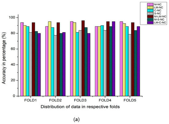
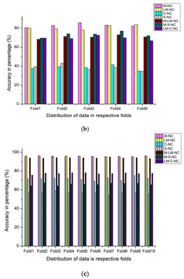
Figure 13.
(a) Fold wise classification accuracies of the DenseNet-161 model implemented on various acoustic features aggregation techniques by using (Strategy-2) on the ESC-10 dataset. (b) Fold wise classification accuracies of the DenseNet-161 model implemented on various acoustic features aggregation techniques by using (Strategy-2) on the ESC-50 dataset. (c) Fold wise classification accuracies of the DenseNet-161 model implemented on various acoustic features aggregation techniques by using (Strategy-2) on the Us8k dataset.
4.4. Performance Evaluation of Proposed New Augmentation Approaches NA-1 and NA-2
After the uncertain and inadequate performance of feature aggregation on the ESC-50 and Us8k datasets, there was a great need to develop a methodology that could produce a state-of-the-art result collectively on all three used Environmental sound datasets. There are very few studies like [81,82], etc., which addressed the ESC-10, ESC-50, and Us8k datasets simultaneously. But these studies were not able to produce up to the mark results. Therefore, there was a strong demand to propose a methodology that could achieve the cutting-edge results concurrently on used environmental sound datasets. This study proposed this approach in which the spectrogram images have been enhanced by consolidating different concepts of audio augmentation, audio to images and then the aggregation of audio extended images with new and Mel filter based original auditory features. The other general group features have not been included for this approach, as their performance for the environmental sound classification task was not satisfactory enough.
The results shown in Table 6 are very promising, as a large amount of data has been regenerated to avoid the risk of overfitting, one of the major causes of lower accuracy in these datasets. The NA-1 attained the best accuracy of 97.98% on Us8k, and NA-2 obtained the highest ever achieved accuracy on ESC datasets with 98.52% on ESC-50 and 99.22% on the ESC-10 datasets. Table 6 exhibits the performance estimation criterion for NA-1 and NA-2 data augmentation approaches. Figure 14a–c display the fold wise accuracy of NA-1 and NA-2 on the executed ESC-10, ESC-50, and Us8k datasets.
Table 6.
The performance evaluation metrics of new data augmentation techniques, NA-1, and NA-2 on used datasets.
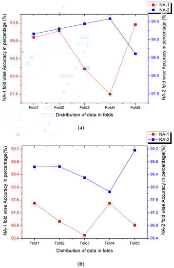
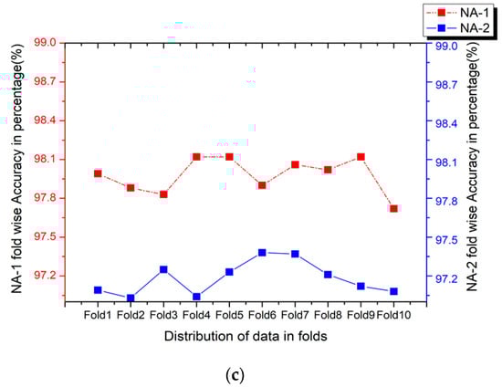
Figure 14.
(a) Fold wise classification accuracies of the DenseNet-161 model implemented on the ESC-10 dataset by implementing NA-1 and NA-2 methodologies. (b) Fold wise classification accuracies of the DenseNet-161 model implemented on the ESC-50 dataset by implementing NA-1 and NA-2 methodologies. (c) Fold wise classification accuracies of the DenseNet-161 model implemented on the Us8k dataset by implementing NA-1 and NA-2 methodologies.
4.5. Performance Assessment of Proposed New Augmentation Approaches NA-1 and NA-2 on Real-Time Audio Data
The real-time audio data has been generated to evaluate the performance of proposed approaches, NA-1 and NA-2. Table 1. briefly explained the details of the real-time data, which has been generated from distinct audio clips from YouTube, considered for validation. The total range of real-time audio clips for ESC-10, ESC-50, and Us8k are 80, 400, and 500, respectively. The distribution of classes in real-time audio data creates one extra fold for the original, ESC-10, ESC-50, and the Us8k datasets. This extra fold was replaced by one-fold from each benchmark dataset, i.e., fold number 5 from ESC-10/ESC-50 was replaced by these real-time dataset folds, and fold number 10 has been substituted with this real-time audio data from the Us8k dataset. The testing method involves the training of all the remaining folds while considering the last fold with real-time audio data as a testing fold. Each time, this testing fold converted into spectrogram images developed by a specific audio feature extraction technique like (Mel, LM, L2M, L3M) and has been tested by a DenseNet-161 on proposed NA-1 and NA-2 approaches. Figure 15 illustrates the accuracy obtained by our considered methods on the real-time environmental sound data. The detailed analysis with the evaluation criterion has been discussed in Table 7. The results demonstrate the brilliant achievement of our recommended NA-1 and NA-2 approaches, even on real-time audio clips taken from YouTube.
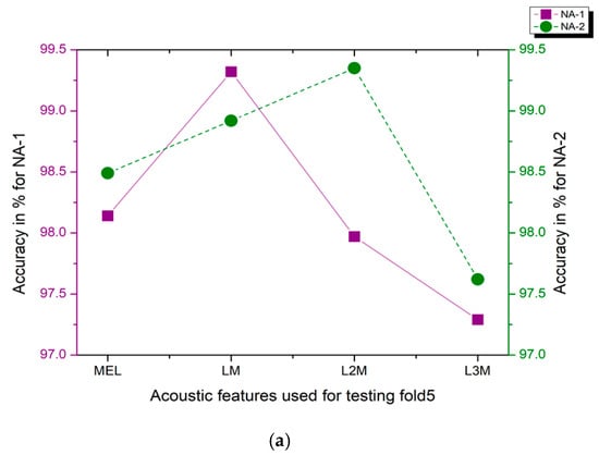
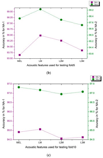
Figure 15.
(a) Evaluation of NA-1 and NA-2 methodologies by replacing testing fold5 with (MEL, LM, L2M, L3M) acoustic features by using (Strategy-2) on the ESC-10 dataset. (b) Evaluation of NA-1 and NA-2 methodologies by replacing testing fold5 with (MEL, LM, L2M, L3M) acoustic features by using (Strategy-2) on the ESC-50 dataset. (c) Evaluation of NA-1 and NA-2 methodologies by replacing testing fold5 with (MEL, LM, L2M, L3M) acoustic features by using (Strategy-2) on the Us8k dataset.
Table 7.
The performance evaluation metrics of real-time audio data for acoustic features (MEL, LM, L2M, L3M) by using new data augmentation approach NA-1 and NA-2 on tested folds of used datasets.
4.6. Comparison and Analysis of Results with Previous and Baseline Methods
In this subsection, a brief comparison between our proposed approach and recent various deep learning models and other related methodologies on the same ESC-10, ESC-50, and Us8k environmental sound classification datasets have been discussed. The comparison has been generated based on two important points. First is the K-fold cross-validation, which is a standard suggested approach from the baseline article. The second point is the direct use of spectrogram images instead of audio clips. The comparative study presented in Table 8 is divided into three subgroups. The first and second group articles originated from the same author that discussed the human and few machine learning algorithms’ accuracies on the ESC-10 and ESC-50 datasets in [38]. The outcomes involve the perception of human beings with the assistance of a crowdsourcing platform called Crowd Flower, some basic machine learning (KNN, SVM), and ensemble models (RF) predictions on the used environmental sound classification datasets. The classification accuracy of the humans has been tested on a total of 4000 judgments for each ESC dataset and achieved an accuracy of 95.7% for the ten category ESC-10 and 81.3% accuracy on 50 category ESC-50 datasets. The sudden decrease in the accuracy was due to the involvement of audio with background noises and some natural soundscapes voices. The same experiment had been evaluated on a few machine learning algorithms, in which the Ensemble model Random Forest obtained 72.7% and 44.3% accuracy on the ESC-10 and ESC-50 datasets, respectively. In [41], the LM that scaled the Mel spectrogram feature was trained on 300 and 150 number of epochs on two layers CNN, which attained an accuracy of 80.5%, 64.9%, and 73.7% on the ESC-10, ESC-50, and Us8k datasets, respectively. When compared with our results, these studies led to a huge marginal difference of 18% in accuracy for each used audio dataset. The third subgroup includes the conversion of audio into spectrogram images and related methodologies. In [83], the spectral images were generated from the audio clips, and these images were in the form of various auditory features (MFCC, CRP, Spectrogram). These images were taken into account for a few famous pre-trained weights AlexNet and GoogleNet. These features were combined in such a way that RGB channels were originated separately from each used acoustic feature. These independent channel images were combined to give a single resultant image. The best-obtained accuracies were 91%, 73%, and 93% for the ESC-10, ESC-50, and Us8k datasets. These accuracies were still 8.22%, 25.52%, and 4.98% less than our best performing proposed method. In [84], the proposed simple CNN architecture and tensor deep stack network, based on the Mel spectrogram images, claimed very low accuracy and was implemented on distinct features accumulation and data enhancement techniques. images, data augmentation techniques by using strategy-2.
Table 8.
Comparison of proposed methodologies (single feature, aggregated features, and augmentation techniques) with other’s published results.
References [31,85] were based upon auditory features aggregation by using deep neural networks. These methodologies show higher results as compared to other executed studies discussed above. Our experimental studies’ results are divided into three parts. First, the best-proposed strategy with a single acoustic feature. Second, the best feature aggregation approach by using the proposed methodology. The final part considers the results by implementing proposed spectrogram.
Table 9 includes those articles that applied different augmentation techniques on audio datasets despite using spectrogram images. Those different strategies comprised pitch shift, adding white noise, and time stretching in [82]; mixing up training samples with each other as a data expansion [26]; time stretching by using slow down and speed up by four factors, negative and positive shift of the pitch, comparison of the dynamic range, mixing up of the recording samples with other background noises sounds clips [86]; the various multiple frequency and time masking on the input spectral images to generate more spectrograms for training [87]. It is evident from the results elaborated in Table 8 and Table 9 that the use of spectrogram images as a feature shows better results compared with the original and augmented audio signals. Our proposed NA-1 and NA-2 new data enhancement techniques, implemented on spectrogram images, attained the highest taxonomic accuracy of 99.22% (NA-2), 98.52% (NA-2), and 97.98% (NA-1) on the ESC-10, ESC-50, and Us8k datasets, respectively. These results are the best-observed outcomes by any rendered study on these datasets.
Table 9.
Other’s audio data augmentation techniques, implemented on the ESC datasets.
5. Conclusions
The major contributions of this manuscript include the introduction of two unprecedented auditory features named L2M and L3M and the involvement of these SIF with Mel and LM to implement two new methodologies named NA-1 and NA-2. The first technique, NA-1, involves the enhancement of SIF data by combining various spectrogram-based audio features. The second approach, NA-2, consists of the vertical aggregation of these images in pairs. The transfer learning-based DenseNet-161 with cyclic learning rate has been implemented on each extended data, individually in the form of SIF. The baseline datasets used in the experiment were ESC-10, ESC-50, and Us8k. The best accuracy for ESC-10 and ESC-50 datasets has been reported by NA-2 methodology, which is 99.22% for ESC-10 and 98.52% for ESC-50. For the Us8k dataset, the NA-1 approach achieved the highest accuracy of 97.98%. These two approaches (NA-1 and NA-2) have also been tested on real-time audio data, generated from YouTube. Their performances on real audio data are also up to the mark. The results produced by the proposed methodology on NA-1 and NA-2 augmented datasets were outstanding on the ESC and Us8k datasets.
The data collection or management is one of the crucial aspects of good performance for any Artificial Intelligence (AI) based system. The less amount of data not only affect the performance of the system but also lead to the problem of overfitting [82]. There are some real-life scenarios in which getting a large number of data in a short interval of time is not practically possible [6,12]. Therefore, such a situation will severely influence the efficiency of the model. Our approach is the combination of two methodologies transfer learning with fine-tuning and features aggregation-based data enhancement techniques. This procedure not only fulfills the requirement of a large amount of data but also prevents the model to train from the scratch. The suggested approach achieves state-of-the-art results with a fewer number of training epochs and less amount of original data. Our proposed methodology attains the highest accuracy rate on used ESC datasets. In the future, we will concentrate on the involvement of other pre-trained weights on features aggregation based on diverse augmentation schemes on ESC datasets.
Author Contributions
Conceptualization, Z.M. and S.-F.S.; Data collection, Z.M.; Formal analysis.; S.-F.S.; Methodology, Z.M.; Project administration, S.-F.S.; Software, Z.M.; Supervision, S.-F.S.; Training, Z.M.; Validation, Z.M.; Visualization, Z.M.; Original draft writing, Z.M.; Review and Editing, Z.M and S.-F.S. All authors have read and agreed to the published version of the manuscript.
Funding
This research received no external funding.
Acknowledgments
The authors would like to praise and thank the respected Editor and Reviewers for their valuable comments and suggestions that enhanced the quality of this manuscript.
Conflicts of Interest
The authors declare no conflict of interest.
References
- Lv, T.; Zhang, H.Y.; Yan, C.H. Double mode surveillance system based on remote audio/video signals acquisition. Appl. Acoust. 2018, 129, 316–321. [Google Scholar] [CrossRef]
- Rabaoui, A.; Davy, M.; Rossignol, S.; Ellouze, N. Using one-class SVMs and wavelets for audio surveillance. IEEE Trans. Inf. Forensics Secur. 2008, 3, 763–775. [Google Scholar] [CrossRef]
- Intani, P.; Orachon, T. Crime warning system using image and sound processing. In Proceedings of the International Conference on Control, Automation and Systems (ICCAS 2013), Gwangju, Korea, 20–23 October 2013; pp. 1751–1753. [Google Scholar]
- Alsouda, Y.; Pllana, S.; Kurti, A. A Machine Learning Driven IoT Solution for Noise Classification in Smart Cities. In Proceedings of the 21st Euromicro Conference on Digital System Design (DSD 2018), Workshop on Machine Learning Driven Technologies and Architectures for Intelligent Internet of Things (ML-IoT), Prague, Czech Republic, 29–31 August 2018; pp. 1–6. [Google Scholar]
- Steinle, S.; Reis, S.; Sabel, C.E. Quantifying human exposure to air pollution-Moving from static monitoring to spatio-temporally resolved personal exposure assessment. Sci. Total Environ. 2013, 443, 184–193. [Google Scholar] [CrossRef] [PubMed]
- Chacón-Rodríguez, A.; Julián, P.; Castro, L.; Alvarado, P.; Hernández, N. Evaluation of gunshot detection algorithms. IEEE Trans. Circuits Syst. I Regul. Pap. 2011, 58, 363–373. [Google Scholar] [CrossRef]
- Vacher, M.; Istrate, D.; Besacier, L.; Serignat, J.; Castelli, E. Sound Detection and Classification for Medical Telesurvey. In Proceedings of the 2014 36th Annual International Conference of the IEEE Engineering in Medicine and Biology Society, Chicago, IL, USA, 26–30 August 2014. [Google Scholar]
- Bhuiyan, M.Y.; Bao, J.; Poddar, B.; Giurgiutiu, V. Toward identifying crack-length-related resonances in acoustic emission waveforms for structural health monitoring applications. Struct. Health Monit. 2018, 17, 577–585. [Google Scholar] [CrossRef]
- Lee, C.H.; Chou, C.H.; Han, C.C.; Huang, R.Z. Automatic recognition of animal vocalizations using averaged MFCC and linear discriminant analysis. Pattern Recognit. Lett. 2006, 27, 93–101. [Google Scholar] [CrossRef]
- Weninger, F.; Schuller, B. Audio recognition in the wild: Static and dynamic classification on a real-world database of animal vocalizations. In Proceedings of the 2011 IEEE International Conference on Acoustics, Speech and Signal Processing (ICASSP), Prague, Czech Republic, 22–27 May 2011; pp. 337–340. [Google Scholar]
- Lee, C.H.; Han, C.C.; Chuang, C.C. Automatic classification of bird species from their sounds using two-dimensional cepstral coefficients. IEEE Trans. Audio Speech Lang. Process. 2008, 16, 1541–1550. [Google Scholar] [CrossRef]
- Baum, E.; Harper, M.; Alicea, R.; Ordonez, C. Sound identification for fire-fighting mobile robots. In Proceedings of the 2018 Second IEEE International Conference on Robotic Computing (IRC), Laguna Hills, CA, USA, 31 January–2 February 2018; Volume 2018, pp. 79–86. [Google Scholar]
- Ciaburro, G. Sound event detection in underground parking garage using convolutional neural network. Big Data Cogn. Comput. 2020, 4, 20. [Google Scholar] [CrossRef]
- Ciaburro, G.; Iannace, G. Improving Smart Cities Safety Using Sound Events Detection Based on Deep Neural Network Algorithms. Informatics 2020, 7, 23. [Google Scholar] [CrossRef]
- Sigtia, S.; Stark, A.M.; Krstulović, S.; Plumbley, M.D. Automatic Environmental Sound Recognition: Performance Versus Computational Cost. IEEE/ACM Trans. Audio Speech Lang. Process. 2016, 24, 2096–2107. [Google Scholar] [CrossRef]
- Sun, L.; Gu, T.; Xie, K.; Chen, J. Text-independent speaker identification based on deep Gaussian correlation supervector. Int. J. Speech Technol. 2019, 22, 449–457. [Google Scholar] [CrossRef]
- Costa, Y.M.G.; Oliveira, L.S.; Silla, C.N. An evaluation of Convolutional Neural Networks for music classification using spectrograms. Appl. Soft Comput. J. 2017, 52, 28–38. [Google Scholar] [CrossRef]
- Phan, H.; Hertel, L.; Maass, M.; Mazur, R.; Mertins, A. Learning representations for nonspeech audio events through their similarities to speech patterns. IEEE/ACM Trans. Audio Speech Lang. Process. 2016, 24, 807–822. [Google Scholar] [CrossRef]
- Crocco, M.; Cristani, M.; Trucco, A.; Murino, V. Audio surveillance: A systematic review. ACM Comput. Surv. 2016, 48. [Google Scholar] [CrossRef]
- Ntalampiras, S.; Potamitis, I.; Fakotakis, N. Probabilistic novelty detection for acoustic surveillance under real-world conditions. IEEE Trans. Multimed. 2011, 13, 713–719. [Google Scholar] [CrossRef]
- Gemmeke, J.F.; Vuegen, L.; Karsmakers, P.; Vanrumste, B.; Van Hamme, H. An exemplar-based NMF approach to audio event detection. In Proceedings of the IEEE Workshop on Applications of Signal Processing to Audio and Acoustics, New Paltz, NY, USA, 20–23 October 2013; pp. 1–4. [Google Scholar]
- Chachada, S.; Kuo, C.C.J. Environmental sound recognition: A survey. APSIPA Trans. Signal Inf. Process. 2014, 3, 1–15. [Google Scholar] [CrossRef]
- Muller, M.; Kurth, F.; Clausen, M. Chroma based statistical audio features for audio matching. In Proceedings of the IEEE Workshop on Applications of Signal Processing to Audio and Acoustics, Bonn, Germany, 16–19 October 2005; pp. 275–278. [Google Scholar]
- Harte, C.; Sandler, M.; Gasser, M. Detecting Harmonic Change in Musical Audio. In Proceedings of the AMCMM’06: The 14th ACM International Conference on Multimedia 2006, Santa Barbara, CA, USA, 23–27 October 2006; pp. 21–25. [Google Scholar]
- Lu, L.; Zhang, H.; Tao, J.; Cui, L.; Jiang, D. Music type classification by spectral contrast feature’. In Proceedings of the IEEE International Conference on Multimedia and Expo, Lausanne, Switzerland, 26–29 August 2002; pp. 113–116. [Google Scholar]
- Zhang, Z.; Xu, S.; Cao, S.; Zhang, S. Deep Convolutional Neural Network with mixup for Environmental Sound Classification. In Chinese Conference on Pattern Recognition and Computer Vision (PRCV); Springer: Cham, Switzerland, 2018; Volume 2, pp. 356–367. [Google Scholar]
- Qu, L.; Weber, C.; Wermter, S. LipSound: Neural mel-spectrogram reconstruction for lip reading. In Proceedings of the Annual Conference of the International Speech Communication Association, INTERSPEECH, Graz, Austria, 15–19 September 2019; Volume 2019, pp. 2768–2772. [Google Scholar]
- Li, J.; Dai, W.; Metze, F.; Qu, S.; Das, S. A Comparison of Deep Learning methods for Environmental Sound Detection. In Proceedings of the IEEE International Conference on Acoustics, Speech, and Signal Processing (ICASSP), New Orleans, LA, USA, 5–9 March 2017; pp. 126–130. [Google Scholar]
- Holdsworth, J.; Nimmo-Smith, I. Implementing a gammatone filter bank. SVOS Final Rep. Part A Audit. Filter Bank 1988, 1, 1–5. [Google Scholar]
- Geiger, J.T.; Helwani, K. Improving event detection for audio surveillance using Gabor filterbank features. In Proceedings of the 2015 23rd European Signal Processing Conference (EUSIPCO), Nice, France, 31 August–4 September 2015; pp. 714–718. [Google Scholar]
- Su, Y.; Zhang, K.; Wang, J.; Zhou, D.; Madani, K. Performance analysis of multiple aggregated acoustic features for environment sound classification. Appl. Acoust. 2020, 158, 107050. [Google Scholar] [CrossRef]
- Yu, C.-Y.; Liu, H.; Qi, Z.-M. Sound Event Detection Using Deep Random Forest. In Proceedings of the Detection and Classification of Acoustic Scenes and Events 2017, Munich, Germany, 16–17 November 2017; pp. 1–3. [Google Scholar]
- Lavner, Y.; Ruinskiy, D. A decision-tree-based algorithm for speech/music classification and segmentation. Eurasip J. Audio Speech Music Process. 2009, 2009, 1–14. [Google Scholar] [CrossRef]
- Karbasi, M.; Ahadi, S.M.; Bahmanian, M. Environmental sound classification using spectral dynamic features. In Proceedings of the ICICS 2011–8th International Conference on Information, Communications and Signal Processing, Singapore, 13–16 December 2011; pp. 1–5. [Google Scholar]
- Aggarwal, S.; Aggarwal, N. Classification of Audio Data using Support Vector Machine. IJCST 2011, 2, 398–405. [Google Scholar]
- Wang, S.; Tang, Z.; Li, S. Design and implementation of an audio classification system based on SVM. Procedia Eng. 2011, 15, 4031–4035. [Google Scholar]
- Tokozume, Y.; Harada, T. Learning Environmental Sounds With End-to-End Convolutional Neural Network. In Proceedings of the 2017 IEEE International Conference on Acoustics, Speech, and Signal Processing (ICASSP), New Orleans, LA, USA, 5–9 March 2017; pp. 2721–2725. [Google Scholar]
- Pons, J.; Serra, X. Randomly Weighted CNNs for (music) audio classification. In Proceedings of the 44th IEEE International Conference on Acoustics, Speech and Signal Processing (ICASSP 2019), Brighton, UK, 12–17 May 2019; pp. 336–340. [Google Scholar]
- Zhao, H.; Huang, X.; Liu, W.; Yang, L. Environmental sound classification based on feature fusion. In MATEC Web of Conferences; EDP Sciences: Ullis, France, 2018; Volume 173, pp. 1–5. [Google Scholar]
- Iannace, G.; Ciaburro, G.; Trematerra, A. Fault diagnosis for UAV blades using artificial neural network. Robotics 2019, 8, 59. [Google Scholar] [CrossRef]
- Piczak, K.J. ESC: Dataset for environmental sound classification. In Proceedings of the MM 2015—Proceedings of the 2015 ACM Multimedia Conference, Brisbane, Australia, 26–30 October 2015; pp. 1015–1018. [Google Scholar]
- Salamon, J.; Jacoby, C.; Bello, J.P. A Dataset and Taxonomy for Urban Sound Research. In Proceedings of the MM ’14 Proceedings of the 22nd ACM International Conference on Multimedia, Orlando, FL, USA, 3–7 November 2014; pp. 1041–1044. [Google Scholar]
- da Silva, B.; Happi, A.W.; Braeken, A.; Touhafi, A. Evaluation of classical Machine Learning techniques towards urban sound recognition on embedded systems. Appl. Sci. 2019, 9, 3885. [Google Scholar] [CrossRef]
- Piczak, K.J. Environmental Sound Classification With Convolutional Neural Networks. In Proceedings of the IEEE International Workshop on Machine Learning for Signal Processing (MLSP), Boston, MA, USA, 17–20 September 2015. [Google Scholar]
- Zhou, H.; Song, Y.; Shu, H. Using deep convolutional neural network to classify urban sounds. In Proceedings of the IEEE Region 10 Annual International Conference, Proceedings/TENCON, Penang, Malaysia, 5–8 November 2017; Volume 2017, pp. 3089–3092. [Google Scholar]
- Demir, F.; Abdullah, D.A.; Sengur, A. A New Deep CNN model for Environmental Sound Classification. IEEE Access 2020, 8, 66529–66537. [Google Scholar] [CrossRef]
- Chen, Y.; Guo, Q.; Liang, X.; Wang, J.; Qian, Y. Environmental sound classification with dilated convolutions. Appl. Acoust. 2019, 148, 123–132. [Google Scholar] [CrossRef]
- Hertel, L.; Phan, H.; Mertins, A. Comparing time and frequency domain for audio event recognition using deep learning. In Proceedings of the 2016 International Joint Conference on Neural Networks (IJCNN), Vancouver, BC, Canada, 24–29 July 2016; pp. 3407–3411. [Google Scholar]
- Pillos, A.; Alghamidi, K.; Alzamel, N.; Pavlov, V.; Machanavajhala, S. A Real-Time Environmental Sound Recognition System for the Android Os. In Proceedings of the Detection and Classification of Acoustic Scenes and Events 2016, Budapest, Hungary, 8 February–7 September 2016. [Google Scholar]
- Ahmad, S.; Agrawal, S.; Joshi, S.; Taran, S.; Bajaj, V.; Demir, F.; Sengur, A. Environmental sound classification using optimum allocation sampling based empirical mode decomposition. Phys. A Stat. Mech. Appl. 2020, 537, 122613. [Google Scholar] [CrossRef]
- Medhat, F.; Chesmore, D.; Robinson, J. Masked Conditional Neural Networks for sound classification. Appl. Soft Comput. J. 2020, 90, 106073. [Google Scholar] [CrossRef]
- Singh, A.; Rajan, P.; Bhavsar, A. SVD-based redundancy removal in 1-D CNNs for acoustic scene classification. Pattern Recognit. Lett. 2020, 131, 383–389. [Google Scholar] [CrossRef]
- Abdoli, S.; Cardinal, P.; Lameiras Koerich, A. End-to-end environmental sound classification using a 1D convolutional neural network. Expert Syst. Appl. 2019, 136, 252–263. [Google Scholar] [CrossRef]
- Li, X.; Chebiyyam, V.; Kirchhoff, K. Multi-stream network with temporal attention for environmental sound classification. In Proceedings of the Annual Conference of the International Speech Communication Association (INTERSPEECH), Graz, Austria, 15–19 September 2019; Volume 2019, pp. 3604–3608. [Google Scholar]
- Ye, J.; Kobayashi, T.; Murakawa, M. Urban sound event classification based on local and global features aggregation. Appl. Acoust. 2017, 117, 246–256. [Google Scholar] [CrossRef]
- Chong, D.; Zou, Y.; Wang, W. Multi-channel Convolutional Neural Networks with Multi-level Feature Fusion for Environmental Sound Classification. In International Conference on Multimedia Modeling; Springer: Cham, Switzerland, 2019; Volume 2, pp. 157–168. [Google Scholar]
- Yang, M.; Yu, L.; Herweg, A. Automated environmental sound recognition for soundscape measurement and assessment. In Proceedings of the INTER-NOISE 2019 MADRID—48th International Congress and Exhibition on Noise Control Engineering, Madrid, Spain, 16–19 June 2019. [Google Scholar]
- Sharma, J.; Granmo, O.-C.; Goodwin, M. Environment Sound Classification using Multiple Feature Channels and Deep Convolutional Neural Networks. J. Latex CL Files 2015, 14, 1–11. [Google Scholar]
- Mushtaq, Z.; Su, S.-F.; Tran, Q.-V. Spectral images based environmental sound classification using CNN with meaningful data augmentation. Appl. Acoust. 2020, 172, 107581. [Google Scholar] [CrossRef]
- Deng, J.D.; Simmermacher, C.; Cranefield, S. A Study on Feature Analysis for Musical Instrument Classification. IEEE Trans. Syst. Man Cybern. Part B Cybern. 2008, 38, 269–274. [Google Scholar] [CrossRef]
- Bachu, R.G.; Kopparthi, S.; Adapa, B.; Barkana, B.D. Separation of Voiced and Unvoiced using Zero crossing rate and Energy of the Speech Signal. In Proceedings of the American Society for Engineering Education, Tulsa, OK, USA, 17–19 September 2008; pp. 279–282. [Google Scholar]
- Bartsch, M.A.; Wakefield, G.H. Audio Thumbnailing of Popular Music Using Chroma-Based Representations. IEEE Trans. Multimed. 2005, 7, 96–104. [Google Scholar] [CrossRef]
- Nepal, A.; Shah, A.K.; Shrestha, D.C. Chroma Feature Extraction. In Encyclopedia of GIS; Springer: Berlin, Germany, 2019; pp. 1–9. [Google Scholar]
- McFee, B.; Raffel, C.; Liang, D.; Ellis, D.; McVicar, M.; Battenberg, E.; Nieto, O. librosa: Audio and Music Signal Analysis in Python. In Proceedings of the 14th Python in Science Conference, Austin, TX, USA, 6–12 July 2015; pp. 18–24. [Google Scholar]
- J. and Others Howard, “vision.learner|fastai,” GitHub. 2018. Available online: https://docs.fast.ai/vision.learner.html (accessed on 26 February 2020).
- Audacity Team, “Audacity,” Audacity Version 2.3.3. 2008. Available online: https://www.audacityteam.org/ (accessed on 20 February 2020).
- Raghu, M.; Zhang, C.; Kleinberg, J.; Bengio, S. Transfusion: Understanding Transfer Learning for Medical Imaging. In Proceedings of the 33rd Conference on Neural Information Processing Systems (NeurlPS 2019), Vancouver, BC, Canada, 8–14 December 2019; pp. 1–11. [Google Scholar]
- Arora, P.; Haeb-Umbach, R. A study on transfer learning for acoustic event detection in a real life scenario. In Proceedings of the 2017 IEEE 19th International Workshop on Multimedia Signal Processing (MMSP), Luton, UK, 16–18 October 2017; pp. 1–6. [Google Scholar]
- Deng, J.; Dong, W.; Socher, R.; Li, L.-J.; Li, K.; Fei-Fei, L. ImageNet: A large-scale hierarchical image database. In Proceedings of the 2019 IEEE Conference on Computer Vision and Pattern Recognition (CVPR), Miami, FL, USA, 20–25 June 2009; pp. 248–255. [Google Scholar]
- Huang, G.; Liu, Z.; van der Maaten, L.; Weinberger, K.Q. Densely Connected Convolutional Networks. In Proceedings of the IEEE Conference on Computer Vision and Pattern Recognition, Honolulu, HI, USA, 21–26 July 2017; Volume 2017, pp. 2261–2269. [Google Scholar]
- Yosinski, J.; Clune, J.; Bengio, Y.; Lipson, H. How transferable are features in deep neural networks? Adv. Neural Inf. Process. Syst. 2014, 4, 3320–3328. [Google Scholar]
- George, A.P.; Powell, W.B. Adaptive stepsizes for recursive estimation with applications in approximate dynamic programming. Mach. Learn. 2006, 65, 167–198. [Google Scholar] [CrossRef]
- Duchi, J.; Hazan, E.; Singer, Y. Adaptive subgradient methods for online learning and stochastic optimization. J. Mach. Learn. Res. 2011, 12, 2121–2159. [Google Scholar]
- Smith, L.N. Cyclical learning rates for training neural networks. In Proceedings of the 2017 IEEE Winter Conference on Applications of Computer Vision, WACV 2017, Santa Rosa, CA, USA, 24–31 March 2017; pp. 464–472. [Google Scholar]
- Wong, S.C.; Gatt, A.; Stamatescu, V.; McDonnell, M.D. Understanding Data Augmentation for Classification: When to Warp? In Proceedings of the International Conference on Digital Image Computing: Techniques and Applications (DICTA), Gold Coast, Australia, 30 November–2 December 2016. [Google Scholar]
- Mikołajczyk, A.; Grochowski, M. Data augmentation for improving deep learning in image classification problem. In Proceedings of the 2018 International Interdisciplinary PhD Workshop (IIPhDW), Swinoujście, Poland, 9–12 May 2018; pp. 117–122. [Google Scholar]
- Wang, S.; Pan, B.; Chen, H.; Ji, Q. Thermal augmented expression recognition. IEEE Trans. Cybern. 2018, 48, 2203–2214. [Google Scholar] [CrossRef]
- Luo, J.; Boutell, M.; Gray, R.T.; Brown, C. Image Transform Bootstrapping and Its Applications to Semantic Scene Classification. IEEE Trans. Syst. Man Cybern. B Cybern. 2005, 35, 563–570. [Google Scholar] [CrossRef]
- Tharwat, A. Classification assessment methods. Appl. Comput. Inform. 2018. [Google Scholar] [CrossRef]
- Chicco, D.; Jurman, G. The advantages of the Matthews correlation coefficient (MCC) over F1 score and accuracy in binary classification evaluation. BMC Genom. 2020, 21, 1–13. [Google Scholar] [CrossRef]
- Demir, F.; Turkoglu, M.; Aslan, M.; Sengur, A. A new pyramidal concatenated CNN approach for environmental sound classification. Appl. Acoust. 2020, 170, 107520. [Google Scholar] [CrossRef]
- Mushtaq, Z.; Su, S.F. Environmental sound classification using a regularized deep convolutional neural network with data augmentation. Appl. Acoust. 2020, 167, 107389. [Google Scholar] [CrossRef]
- Boddapati, V.; Petef, A.; Rasmusson, J.; Lundberg, L. Classifying environmental sounds using image recognition networks. Procedia Comput. Sci. 2017, 112, 2048–2056. [Google Scholar] [CrossRef]
- Khamparia, A.; Gupta, D.; Nguyen, N.G.; Khanna, A.; Pandey, B.; Tiwari, P. Sound classification using convolutional neural network and tensor deep stacking network. IEEE Access 2019, 7, 7717–7727. [Google Scholar] [CrossRef]
- Su, Y.; Zhang, K.; Wang, J.; Madani, K. Environment sound classification using a two-stream CNN based on decision-level fusion. Sensors 2019, 19, 1733. [Google Scholar] [CrossRef]
- Salamon, J.; Bello, J.P. Deep Convolutional Neural Networks and Data Augmentation for Environmental Sound Classification. IEEE Signal Process. Lett. 2017, 24, 279–283. [Google Scholar] [CrossRef]
- Zhang, Z.; Xu, S.; Zhang, S.; Qiao, T.; Cao, S. Learning Attentive Representations for Environmental Sound Classification. IEEE Access 2019, 7, 130327–130339. [Google Scholar] [CrossRef]
- Tokozume, Y.; Ushiku, Y.; Harada, T. Learning from Between-class Examples for Deep Sound Recognition. In Proceedings of the 6th International Conference on Learning Representations (ICLR), Vancouver, BC, Canada, 30 April–3 May 2018; pp. 1–13. [Google Scholar]


Publisher’s Note: MDPI stays neutral with regard to jurisdictional claims in published maps and institutional affiliations. |
© 2020 by the authors. Licensee MDPI, Basel, Switzerland. This article is an open access article distributed under the terms and conditions of the Creative Commons Attribution (CC BY) license (http://creativecommons.org/licenses/by/4.0/).