A Novel MCDM Method Based on Plithogenic Hypersoft Sets under Fuzzy Neutrosophic Environment

Abstract

In this paper, we advance the study of plithogenic hypersoft set (PHSS). We present four classifications of PHSS that are based on the number of attributes chosen for application and the nature of alternatives or that of attribute value degree of appurtenance. These four PHSS classifications cover most of the fuzzy and neutrosophic cases that can have neutrosophic applications in symmetry. We also make explanations with an illustrative example for demonstrating these four classifications. We then propose a novel multi-criteria decision making (MCDM) method that is based on PHSS, as an extension of the technique for order preference by similarity to an ideal solution (TOPSIS). A number of real MCDM problems are complicated with uncertainty that require each selection criteria or attribute to be further subdivided into attribute values and all alternatives to be evaluated separately against each attribute value. The proposed PHSS-based TOPSIS can be used in order to solve these real MCDM problems that are precisely modeled by the concept of PHSS, in which each attribute value has a neutrosophic degree of appurtenance corresponding to each alternative under consideration, in the light of some given criteria. For a real application, a parking spot choice problem is solved by the proposed PHSS-based TOPSIS under fuzzy neutrosophic environment and it is validated by considering two different sets of alternatives along with a comparison with fuzzy TOPSIS in each case. The results are highly encouraging and a MATLAB code of the algorithm of PHSS-based TOPSIS is also complied in order to extend the scope of the work to analyze time series and in developing algorithms for graph theory, machine learning, pattern recognition, and artificial intelligence.

1. Introduction

A strong mathematical tool is always needed in order to combat real world problems involving uncertainty in the data. This necessity has urged scholars to introduce different mathematical tools to facilitate the world for solving such problems. In 1965, the concept of fuzzy set was introduced by Zadeh [1], in which each element is assigned a membership degree in the form of a single crisp value in the interval $[0,1]$. It has been studied extensively by the researchers and a number of real life problems have been solved by fuzzy sets [2,3,4,5]. However, in some practical situations, it is seen that this membership degree is hard to be defined by a single number. The uncertainty in the membership degree became the cause to introduce the concept of interval-valued fuzzy set in which the degree of membership is an interval value in $[0,1]$. Later on, the concept of intuitionistic fuzzy set (IFS) was proposed by Atanassov [6] in 1986, which incorporates the non-membership degree. IFS had many applications [7,8,9,10].

However, IFS is unable to deal with indeterminate information, which is very common in belief systems. This inadequacy was addressed by Smarandache [11] in 2000, who introduced the concept of neutrosophic set in which membership (T), indeterminacy (I) and non-membership (F) degrees were independently quantified i.e., $\mathrm{T},\mathrm{I},\mathrm{F}\in [0,1]$ and the sum $\mathrm{T}+\mathrm{I}+\mathrm{F}$ need not to be contained in $[0,1]$. All of these mathematical tools have been thoroughly explored and successfully applied to deal with uncertainties [12,13,14,15], yet these tools usually fail to handle uncertainty in a variety of practical situation, because these tools require all notions to be exact and do not possess a parametrization tool. Consequently, soft set was introduced by Molodstsov [16] in 1999, which can be regarded as a general mathematical tool to deal with uncertainty. Molodstsov [16] defined soft set as a parameterized family of subsets of a universe of discourse. In 2003, Maji et al. [17] introduced aggregation operations on soft sets. Soft sets and their hybrids have been successfully applied in various areas [18,19,20,21].

In a variety of real life MCDM problems, the attributes need to be further sub-divided into attribute values for a better decision. This need was fulfilled by Smarandache [22], who introduced the concept of hypersoft set as a generalization of the concept of soft set in 2018. Besides, Smarandache [22] introduced the concept of plithogenic hypersoft set with crisp, fuzzy, intuitionistic fuzzy, neutrosophic, and plithogenic sets. In 2020, Saeed et al. [23] presented a study on the fundamentals of hypersoft set theory. Smarandache [24,25] developed the aggregation operations on plithogenic set and proved that the plithogenic set is the most generalized structure that can be efficiently applied to a variety of real life problems [26,27,28,29].

A PHSS-based TOPSIS is proposed in the article to deal with MCDM problem, in which attribute may have attribute values and each attribute value has a neutrosophic degree of appurtenance of each alternative. The proposed method is authenticated by taking two different sets of alternatives. A comparison with fuzzy TOPSIS is made in each case. It shows that the results are highly inspiring. A MATLAB code of the algorithm of PHSS-based TOPSIS is also complied in order to encompass the scope of the work to analyze time series and in developing algorithms for graph theory, artificial intelligence, machine learning, pattern recognition, and neutrosophic applications in symmetry. It appears quite pertinent to point out that the article gives detailed insight on PHSS with related definitions and its implementation in MCDM process. The scope of the work can be extended in other mathematics directions as well by introducing important theorems and propositions [24].

The remainder of this article is organized, as follows. In Section 2, we briefly review some basic notions, leading to the definitions of soft sets, hypersoft sets, plithogenic sets, and plithogenic hypersoft sets (PHSSs), along with an illustrative example. Section 3 consists of the four proposed classifications of PHSSs based on different criteria. More explanations with an illustrative example for the four classifications are also made. In Section 4, the algorithm of the proposed PHSS-based TOPSIS is given, along with its application to a real life parking spot choice problem under fuzzy neutrosophic environment and its comparison with fuzzy TOPSIS. Section 5 provides the conclusion and future directions.

2. Preliminaries

This section comprises of some necessary basic concepts that are related to plithogenic hypersoft set (PHSS), which is also defined in this section along with an illustrative example for a clear understanding. Throughout the study, let $\mathcal{U}$ be a non-empty universal set, $P\left(\mathcal{U}\right)$ be the power set of $\mathcal{U}$, $X\subseteq \mathcal{U}$ be a finite set of alternatives, and $\mathcal{A}$ be a finite set of n distinct parameters or attributes, as given by

$$\begin{array}{c}\hfill \mathcal{A}=\{a_1,a_2,\cdots ,a_n\},n\ge 1.\end{array}$$

The attribute values of $a_1,a_2,\cdots ,a_n$ belong to the sets $A_1,A_2,\dots ,A_n$, respectively, where $A_i\cap A_j=\varphi$, for $i\ne j$, and $i,j\in \{1,2,\dots ,n\}$. Moreover, we consider a finite number of uni-dimensional attributes and each attribute has a finite discrete set of attribute values. However, it is worth mentioning that the attributes may have an infinite number of attribute values. In such a case, every structure with non-Archimedean metrics can be dealt in depth [30,31].

2.1. Soft Sets

A soft set over $\mathcal{U}$ is a mapping $\mathcal{F}:\mathcal{B}\to P\left(\mathcal{U}\right)$, $\mathcal{B}\subseteq \mathcal{A}$ with the value ${\mathcal{F}}_{\mathcal{B}}\left(\alpha \right)\in P\left(\mathcal{U}\right)$ at $\alpha \in \mathcal{B}$ and ${\mathcal{F}}_{\mathcal{B}}\left(\alpha \right)=\varphi$ if $\alpha \notin \mathcal{B}$. It is denoted by $(\mathcal{F},\mathcal{B})$ and written as follows [16]:

$$\begin{array}{c}\hfill (\mathcal{F},\mathcal{B})=\{(\alpha ,{\mathcal{F}}_{\mathcal{B}}\left(\alpha \right)):\alpha \in \mathcal{B},{\mathcal{F}}_{\mathcal{B}}\left(\alpha \right)\in P\left(\mathcal{U}\right)\}.\end{array}$$

Moreover, a soft set over $\mathcal{U}$ can be regarded as a parameterized family of the subsets of $\mathcal{U}$. For an attribute $\alpha \in \mathcal{B}$, ${\mathcal{F}}_{\mathcal{B}}\left(\alpha \right)$ is considered as the set of $\alpha$-approximate elements of the soft set $(\mathcal{F},\mathcal{B})$.

2.2. Hypersoft Sets

Let C denote the cartesian product of the sets $A_1,A_2,\dots ,A_n$, i.e., $C=A_1\times A_2\times \dots \times A_n,n\ge$ 1. Subsequently, a hypersoft set $(\mathcal{H},\mathcal{C})$ over $\mathcal{U}$ is a mapping defined by $\mathcal{H}:C\to P\left(\mathcal{U}\right)$ [22]. For an n-tuple $({\gamma }_1,{\gamma }_2,\dots ,{\gamma }_n)\in C,$, where ${\gamma }_i\in A_i,i=1,2,3,\dots ,n$, a hypersoft set is written as

$$\begin{array}{c}\hfill (\mathcal{H},\mathcal{C})=\{(\gamma ,\mathcal{H}\left(\gamma \right)):\gamma =({\gamma }_1,{\gamma }_2,\dots ,{\gamma }_n)\in \mathcal{C},\mathcal{H}\left(\gamma \right)\in P\left(\mathcal{U}\right)\}.\end{array}$$

It may be noted that hypersoft set is a generalization of soft set.

2.3. Plithogenic Sets

A set X is called a plithogenic set if all of its members are characterized by the attributes under consideration and each attribute may have any number of attribute values [24]. Each attribute value possesses a corresponding appurtenance degree of the element x, to the set X, with respect to some given criteria. Moreover, a contradiction degree function is defined between each attribute value and the dominant attribute value of an attribute in order to obtain accuracy for aggregation operations on plithogenic sets. These degrees of appurtenance and contradiction may be fuzzy, intuitionistic fuzzy or neutrosophic degrees.

Remark 1.

Plithogenic set is regarded as a generalization of crisp, fuzzy, intuitionistic fuzzy. and neutrosophic sets, since the elements of later sets are characterized by a combined single attribute value (degree of appurtenance), which has only one value for crisp and fuzzy sets i.e., membership, two values in case of intuitionistic fuzzy set i.e., membership and non-membership, and three values for neutrosophic set i.e., membership, indeterminacy, and non-membership. In the case of plithogenic set, each element is separately characterized by all attribute values under consideration in terms of degree of appurtenance.

2.4. Plithogenic Hypersoft Set (PHSS)

Let $X\subseteq \mathcal{U}$ and $C=A_1\times A_2\times \dots \times A_n$, where $n\ge 1$ and $A_i$ is the set of all attribute values of the attribute $a_i$, $i=1,2,3,\dots ,n$. Each attribute value $\gamma$ possesses a corresponding appurtenance degree $d(x,\gamma )$ of the member $x\in X$, in accordance with some given condition or criteria. The attribute value degree of appurtenance is a function that is defined by

$$\begin{array}{c}\hfill d:X\times C\to P({[0,1]}^j),\forall x\in X,\end{array}$$

such that $d(x,\gamma )\in {[0,1]}^j$, and $P\left({[0,1]}^j\right)$ is the power set of ${[0,1]}^j$, where $j=1,2,3$ are for fuzzy, intuitionistic fuzzy, and neutrosophic degree of appurtenance, respectively.

Furthermore, the degree of contradiction (dissimilarity) between any two attribute values of the same attribute is a function given by

$$c:A_i\times A_i\to P\left({[0,1]}^j\right),1\le i\le n,j=1,2,3.$$

For any two attribute values ${\gamma }_1$ and ${\gamma }_2$ of the same attribute, it is denoted by $c({\gamma }_1,{\gamma }_2)$ and satisfies the following axioms:

$$\begin{array}{c}\hfill c({\gamma }_1,{\gamma }_1)=0,\\ \hfill c({\gamma }_1,{\gamma }_2)=c({\gamma }_2,{\gamma }_1).\end{array}$$

Subsequently, $(X,\mathcal{A},C,d,c)$ is called a plithogenic hypersoft set (PHSS) [22]. For an n-tuple $({\gamma }_1,{\gamma }_2,\dots ,{\gamma }_n)\in C,$${\gamma }_i\in A_i,1\le i\le n$, a plithogenic hypersoft set $F:C\to P\left(\mathcal{U}\right)$ is mathematically written as

$$\begin{array}{c}\hfill \begin{array}{c}\hfill F\left(\{{\gamma }_1,{\gamma }_2,\dots ,{\gamma }_n\}\right)=\{x(d_x\left({\gamma }_1\right),d_x\left({\gamma }_2\right),\dots ,d_x\left({\gamma }_n\right)),x\in X\}.\end{array}\end{array}$$

Remark 2.

Plithogenic hypersoft set is a generalization of crisp hypersoft set, fuzzy hypersoft set, intuitionistic fuzzy hypersoft set, and neutrosophic hypersoft set.

2.5. Illustrative Example

Let $\mathcal{U}=\{m_1,m_2,m_3,\dots ,m_{10}\}$ be a universe containing mobile phones. A person wants to buy a mobile phone for which the mobile phones under consideration (alternatives) are contained in $X\subseteq \mathcal{U}$, given by

$$\begin{array}{c}\hfill X=\{m_2,m_3,m_5,m_8\}.\end{array}$$

The characteristics or attributes of the mobile phones belong to the set $\mathcal{A}=\{a_1,a_2,a_3,a_4\}$, such that

• $a_1$ = Processor power,
• $a_2$ = RAM,
• $a_3$ = Front camera resolution,
• $a_4$ = Screen size in inches.

The attribute values of $a_1,a_2,a_3,a_4$ are contained in the sets $A_1,A_2,A_3,A_4$ given below.

• $A_1=\{$ dual-core, quad-core, octa-core},
• $A_2=\{$2GB, 4GB, 8GB, 16GB},
• $A_3=\{$2MP, 5MP, 8MP, 16MP},
• $A_4=\{$4, 4.5, 5, 5.5, 6}.

1. 

Soft set

Consider $\mathcal{B}=\{a_2,a_3\}\subseteq \mathcal{A}$. Afterwards, a soft set $(\mathcal{F},\mathcal{B})$, defined by the mapping $\mathcal{F}:\mathcal{B}\to P\left(\mathcal{U}\right)$, is given by

$$(\mathcal{F},\mathcal{B})=\{(a_2,\{m_2,m_5\}),(a_3,\{m_2,m_3,m_8\})\}$$

Element-wise, it may be written as

$$\begin{array}{c}\hfill {\mathcal{F}}_{\mathcal{B}}\left(a_2\right)=\{m_2,m_5\},{\mathcal{F}}_{\mathcal{B}}\left(a_3\right)=\{m_2,m_3,m_8\}.\end{array}$$

2. 

Hypersoft set

Let $C=A_1\times A_2\times A_3\times A_4$. Then, a hypersoft set over $\mathcal{U}$ is a function $f:C\to P\left(\mathcal{U}\right)$. For an element $\left(\mathrm{octa}\text{-}\mathrm{core},8\mathrm{GB},16\mathrm{MP},5.5\right)\in C$, it is given by

$$\begin{array}{c}\hfill f\left(\left\{\mathrm{octa}\text{-}\mathrm{core},8\mathrm{GB},16\mathrm{MP},5.5\right\}\right)=\{m_5,m_8\}\end{array}$$

3. 

Plithogenic hypersoft set

For the same tuple $\left(\mathrm{octa}\text{-}\mathrm{core},8\mathrm{GB},16\mathrm{MP},5.5\right)\in C$, a plithogenic hypersoft set $F:C\to P\left(\mathcal{U}\right)$ is given by

$$\begin{array}{c}\hfill \begin{array}{cc}\hfill F\left(\right\{\mathrm{octa}\text{-}\mathrm{core},8\mathrm{GB},16\mathrm{MP},5.5\left\}\right)=& \{m_5\left(d_{m_5}\left(\mathrm{octa}\text{-}\mathrm{core}\right),d_{m_5}\left(8\mathrm{GB}\right),d_{m_5}\left(16\mathrm{MP}\right),d_{m_5}\left(5.5\right)\right),\hfill \\ & m_8\left(d_{m_8}\left(\mathrm{octa}\text{-}\mathrm{core}\right),d_{m_8}\left(8\mathrm{GB}\right),d_{m_8}\left(16\mathrm{MP}\right),d_{m_8}\left(5.5\right)\right)\},\hfill \end{array}\end{array}$$

where $d_{m_5}\left(\gamma \right)$ stands for the degree of appurtenance of the attribute value $\gamma \in \left(\mathrm{octa}\text{-}\mathrm{core},8\mathrm{GB},16\mathrm{MP},5.5\right)$ to the element $m_5\in X$. A similar meaning applies to $d_{m_8}\left(\gamma \right)$.

3. The Four Classifications of PHSS

In this section, we propose the four different classifications of PHSS that are based on the number of attributes chosen for application and the characteristics of alternatives under consideration or that of the attribute value degree of appurtenance function. The same example from Section 2 is considered to each classification for a practical understanding. Figure 1 shows a diagram for these classifications.

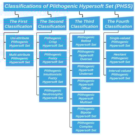
Figure 1. Flowchart of four classifications of plithogenic hypersoft sets (PHSS).

3.1. The First Classification

This classification is based on the number of attributes that are chosen by the decision makers for application.

3.1.1. Uni-Attribute Plithogenic Hypersoft Set

Let $\alpha \in \mathcal{A}$ be an attribute required by the experts for application purpose and the attribute values of $\alpha$ belong to the finite discrete set $Y=\{y_1,y_2,\dots ,y_m\}$, $m\ge 1$. Hence, the degree of appurtenance function is given by

$$\begin{array}{c}\hfill d:X\times Y\to P\left({[0,1]}^j\right),\forall x\in X,\end{array}$$

such that $d(x,y)\subseteq {[0,1]}^j$, where $P\left({[0,1]}^j\right)$ denotes the power set of ${[0,1]}^j$ and $j=1,2,3$ stands for fuzzy, intuitionistic fuzzy, or neutrosophic degree of appurtenance, respectively.

The contradiction degree function between any two attribute values of $\alpha$, is given by

$$c:Y\times Y\to P\left({[0,1]}^j\right),\forall y\in Y,j=1,2,3.$$

For any two attribute values $y_1,y_2\in Y$, it is denoted by $c(y_1,y_2)$ and the following properties hold:

$$\begin{array}{c}\hfill c(y_1,y_1)=0,\\ \hfill c(y_1,y_2)=c(y_2,y_1).\end{array}$$

Subsequently, $(X,\alpha ,Y,d,c)$ is termed as a uni-attribute plithogenic hypersoft set. For an attribute value $y\in Y$, a uni-attribute plithogenic hypersoft set $F:Y\to P\left(\mathcal{U}\right)$ is mathematically written as

$$\begin{array}{c}\hfill F\left(y\right)=\{x\left(d_x\left(y\right)\right):x\in X\}.\end{array}$$

3.1.2. Multi-Attribute Plithogenic Hypersoft Set

Consider a subset $\mathcal{B}$ of $\mathcal{A}$, consisting of all attributes that were chosen by the experts, given by

$$\mathcal{B}=\{b_1,b_2,\dots ,b_m\},m>1.$$

Let the attribute values of $b_1,b_2,\dots ,b_m$ belong to the sets $B_1,B_2,\dots ,B_m$, respectively, and

$$\begin{array}{c}\hfill Y_m=B_1\times B_2\times \dots \times B_m.\end{array}$$

Afterwards, the appurtenance degree function is

$$\begin{array}{c}\hfill d:X\times Y_m\to P\left({[0,1]}^j\right),\forall x\in X,\end{array}$$

such that $d(x,y)\subseteq {[0,1]}^j$, $j=1,2,3$. In this case, the contradiction degree function is given by

$$c:B_i\times B_i\to P\left({[0,1]}^j\right),1\le i\le m,j=1,2,3.$$

The degree of contradiction between any two attribute values $y_1$ and $y_2$, is denoted by $c(y_1,y_2)$ and it satisfies the following axioms:

$$\begin{array}{c}\hfill c(y_1,y_1)=0,\\ \hfill c(y_1,y_2)=c(y_2,y_1).\end{array}$$

Subsequently, $(X,\mathcal{B},Y_m,d,c)$ is called a multi-attribute plithogenic hypersoft set. For an m-tuple $(y_1,y_2,\dots ,y_m)\in Y_m,$$y_i\in B_i,1\le i\le m$, a multi-attribute plithogenic hypersoft set $F:Y_m\to P\left(\mathcal{U}\right)$ is mathematically written as

$$\begin{array}{c}\hfill \begin{array}{c}\hfill F\left(\{y_1,y_2,\dots ,y_m\}\right)=\{x(d_x\left(y_1\right),d_x\left(y_2\right),\dots ,d_x\left(y_m\right)),x\in X\}.\end{array}\end{array}$$

Example 1.

Consider the previous example in which $\mathcal{U}=\{m_1,m_2,m_3,\dots ,m_{10}\}$ and $X\subseteq \mathcal{U}$ is given by $X=\{m_2,m_3,m_5,m_8\}$. The attributes belong to the set $\mathcal{A}=\{a_1,a_2,a_3,a_4\}$, such that

$a_1$ = Processor power,

$a_2$ = RAM,

$a_3$ = Front camera resolution,

$a_4$ = Screen size in inches.

The attribute values of $a_1,a_2,a_3,a_4$ are contained in the sets $A_1,A_2,A_3,A_4$ given below:

$A_1=\{$ dual-core, quad-core, octa-core},

$A_2=\{$2GB, 4GB, 8GB, 16GB},

$A_3=\{$2MP, 5MP, 8MP, 16MP},

$A_4=\{$4, 4.5, 5, 5.5, 6}.

1. 

Uni-attribute plithogenic hypersoft set

Consider the most demanding feature of a mobile phone given by the attribute $a_3$ that stands for front camera resolution. The set of attribute values of $a_3$ is $A_3=\left\{2\mathrm{MP},5\mathrm{MP},8\mathrm{MP},16\mathrm{MP}\right\}$. Then, the uni-attribute plithogenic hypersoft set $F:A_3\to P\left(\mathcal{U}\right)$ is given by

$$\begin{array}{c}\hfill F\left(\gamma \right)=\{x\left(d_x\left(\gamma \right)\right),\forall \gamma \in A_3,x\in X\},\end{array}$$

where $d_x\left(\gamma \right)$ denotes the degree of appurtenance of $x\in X$, to the set X, w.r.t. the attribute value $\gamma \in A_3$. For an attribute value 16MP $\in A_3$, we have

$$\begin{array}{c}\hfill F\left(16\mathrm{MP}\right)=\{m_5\left(d_{m_5}\left(16\mathrm{MP}\right)\right),m_8\left(d_{m_8}\left(16\mathrm{MP}\right)\right)\},\end{array}$$

2. 

Multi-attribute plithogenic hypersoft set

Let $\mathcal{B}=\{a_3,a_4\}$ be the set of attributes required by the customer. Therefore, we need $A_3$ and $A_4$ given by

$$\begin{array}{cc}\hfill & A_3=\left\{2\mathrm{MP},5\mathrm{MP},8\mathrm{MP},16\mathrm{MP}\right\},\\ \hfill & A_4=\{4,4.5,5,5.5,6\}.\end{array}$$

Suppose that the customer is interested to buy a mobile phone with specific requirements of 16MP front camera with 5.5 inch screen size. In this case, we take $(16\mathrm{MP},5.5)\in A_3\times A_4$ and a multi-attribute plithogenic hypersoft set $F:A_3\times A_4\to P\left(\mathcal{U}\right)$ is given by

$$\begin{array}{c}\hfill \begin{array}{c}\hfill F\left(\{16\mathrm{MP},5.5\}\right)=\{m_5\left(d_{m_5}\left(16\mathrm{MP}\right),d_{m_5}\left(5.5\right)\right),m_8\left(d_{m_8}\left(16\mathrm{MP}\right),d_{m_8}\left(5.5\right)\right)\},\end{array}\end{array}$$

where $d_{m_5}\left(\gamma \right)$ stands for the degree of appurtenance of $m_5$ to the set X w.r.t. the attribute value $\gamma \in (16\mathrm{MP},5.5)$.

3.2. The Second Classification

This classification is based on the nature of the attribute value degree of appurtenance that may be crisp, fuzzy, intuitionistic fuzzy, or neutrosophic degree of appurtenance.

3.2.1. Plithogenic Crisp Hypersoft Set

A plithogenic hypersoft set X is crisp if the appurtenance degree $d_x\left(\gamma \right)$ of each member $x\in X$, w.r.t. each attribute value $\gamma$, is crisp, i.e., $d_x\left(\gamma \right)$ is either 0 or 1.

3.2.2. Plithogenic Fuzzy Hypersoft Set

If the appurtenance degree $d_x\left(\gamma \right)$ of each member $x\in X$, w.r.t. each attribute value $\gamma$, is fuzzy, then it is called the plithogenic fuzzy hypersoft set. Mathematically, $d_x\left(\gamma \right)\in P\left([0,1]\right)$.

3.2.3. Plithogenic Intuitionistic Fuzzy Hypersoft Set

If the attribute value appurtenance degree $d_x\left(\gamma \right)$ of each $x\in X$, w.r.t. each attribute value, is intuitionistic fuzzy degree, then it is called the plithogenic intuitionistic fuzzy hypersoft set. Mathematically, it is written as $d_x\left(\gamma \right)\in P\left({[0,1]}^2\right)$.

3.2.4. Plithogenic Neutrosophic Hypersoft Set

A plithogenic hypersoft set X is called plithogenic neutrosophic hypersoft set if $d_x\left(\gamma \right)\in P\left({[0,1]}^3\right)$.

Example 2.

For$\left(\mathit{octa}\text{-}\mathit{core},\mathit{8}\mathit{GB},\mathit{16}\mathit{MP},\mathit{5.5}\right)\in C$, we have the following results:

1. 

Plithogenic crisp hypersoft set

$$\begin{array}{c}\hfill \begin{array}{c}\hfill F\left(\left\{\mathit{octa}\text{-}\mathit{core},\mathit{8}\mathit{GB},\mathit{16}\mathit{MP},\mathit{5.5}\right\}\right)=\{m_5(1,1,1,1),m_8(1,1,1,1)\}.\end{array}\end{array}$$

2. 

Plithogenic fuzzy hypersoft set

$$\begin{array}{c}\hfill \begin{array}{c}\hfill F\left(\left\{\mathit{octa}\text{-}\mathit{core},\mathit{8}\mathit{GB},\mathit{16}\mathit{MP},\mathit{5.5}\right\}\right)=\{m_5(0.9,0.2,1,0.75),m_8(0.5,0.5,0.25,0.9)\}.\end{array}\end{array}$$

3. 

Plithogenic intuitionistic fuzzy hypersoft set

$$\begin{array}{c}\hfill \begin{array}{cc}\hfill F\left(\right\{\mathit{octa}\text{-}\mathit{core},\mathit{8}\mathit{GB},\mathit{16}\mathit{MP},\mathit{5.5}\left\}\right)=& \{m_5\left((0.9,0.1),(0.2,0.6),(1,0),(0.75,0.1)\right),\hfill \\ & m_8((0.5,0.25),(0.5,0.5),(0.25,0.1),(0.9,0))\}.\hfill \end{array}\end{array}$$

4. 

Plithogenic neutrosophic hypersoft set

$$\begin{array}{c}\hfill \begin{array}{cc}\hfill F\left(\right\{\mathit{octa}\text{-}\mathit{core},\mathit{8}\mathit{GB},\mathit{16}\mathit{MP},\mathit{5.5}\left\}\right)=& \{m_5((0.9,0.7,0.1),(0.2,0.3,0.6),(1,0.25,0),(0.75,0.3,0.1)),\hfill \\ & m_8((0.5,1,0.25),(0.5,0.9,0.5),(0.25,0.7,0.1),(0.9,0.8,0))\}.\hfill \end{array}\end{array}$$

3.3. The Third Classification

This classification is based on the properties of attribute values and degree of appurtenance function.

3.3.1. Plithogenic Refined Hypersoft Set

Let $(X,\mathcal{A},C,d,c)$ be a plithogenic hypersoft set and A denote the set of attribute values of an attribute a. If an attribute value $\gamma \in A$ of the attribute a is subdivided or split into at least two or more attribute sub-values ${\gamma }_1,{\gamma }_2,{\gamma }_3,\dots \in A$, such that the attribute sub-value degree of appurtenance function $d(x,{\gamma }_i)\in P\left({[0,1]}^j\right)$, for $i=1,2,3,\cdots$ and $j=1,2,3$ for fuzzy, intuitionistic fuzzy, neutrosophic degree of appurtenance, respectively, then X is called a refined plithogenic hypersoft set. It is represented as $(X_r,\mathcal{A},C,d,c)$.

3.3.2. Plithogenic Hypersoft Overset

If the degree of appurtenance of any element $x\in X$ w.r.t. any attribute value $\gamma \in A$ of an attribute a is greater than 1, i.e., $d(x,\gamma )>1$, then X is called a plithogenic hypersoft overset. It is represented as $(X_o,\mathcal{A},C,d,c)$.

3.3.3. Plithogenic Hypersoft Underset

If the degree of appurtenance of any element $x\in X$ w.r.t. any attribute value $\gamma \in A$ of an attribute a less than 0, i.e., $d(x,\gamma )<0$, then X is called a plithogenic hypersoft underset. It is represented as $(X_u,\mathcal{A},C,d,c)$.

3.3.4. Plithogenic Hypersoft Offset

A plithogenic hypersoft set $(X,\mathcal{A},C,d,c)$ is called a plithogenic hypersoft offset if it is both an overset and an underset. Mathematically, if $d(x_1,{\gamma }_1)>1$ and $d(x_2,{\gamma }_2)<0$ for the same or different attribute values ${\gamma }_1,{\gamma }_2\in A$ that correspond to the same or different members $x_1,x_2\in X$, then $(X_{\mathrm{off}},\mathcal{A},C,d,c)$ is a plithogenic hypersoft offset.

3.3.5. Plithogenic Hypersoft Multiset

If an element $x\in X$ repeats itself into the set X with same plithogenic components given by

$$x(c_1,c_2,\dots ,c_n),x(c_1,c_2,\dots ,c_n),$$

or with different plithogenic components given by

$$x(c_1,c_2,\dots ,c_n),x(d_1,d_2,\dots ,d_n),$$

then $(X_n,\mathcal{A},C,d,c)$ is called a plithogenic hypersoft multiset.

3.3.6. Plithogenic Bipolar Hypersoft Set

If the attribute value appurtenance degree function is given by

$$\begin{array}{c}\hfill d:X\times C\to P\left({[-1,0]}^j\right)\times P\left({[0,1]}^j\right),\forall x\in X,\end{array}$$

where $j=1,2,3,$ then, $(X_b,\mathcal{A},C,d,c)$ is called plithogenic bipolar hypersoft set. It may be noted that, for an attribute value $\gamma$, $d(x,\gamma )$ allots a negative degree of appurtenance in $[-1,0]$ and a positive degree of appurtenance in $[0,1]$ to each element $x\in X$ with respect to each attribute value $\gamma$.

Remark 3.

The concept of plithogenic bipolar hypersoft set can be extended to plithogenic tripolar hypersoft set and so on up to plithogenic multipolar hypersoft set.

3.3.7. Plithogenic Complex Hypersoft Set

If for any $x\in X$, the attribute value appurtenance degree function, with respect to any attribute value $\gamma$, is given by

$$\begin{array}{c}\hfill d:X\times C\to P\left({[0,1]}^j\right)\times P\left({[0,1]}^j\right),j=1,2,3,\end{array}$$

such that $d(x,\gamma )$ is a complex number of the form $c_1.e^{i{c}_2}$, where $c_1$ (amplitude) and $c_2$ (phase) are subsets of $[0,1]$, then $(X_{\mathrm{com}},\mathcal{A},C,d,c)$ is called a plithogenic complex hypersoft set.

Example 3.

Consider the same example of choosing a suitable mobile phone from the set $X=\{m_2,m_3,m_5,m_8\}$. The attributes are $a_1,a_2,a_3,a_4$, whose attribute values are contained in the sets $A_1,A_2,A_3,A_4$.

1. 

Plithogenic refined hypersoft set

Consider an attribute $a_4$ = $\mathrm{screen}\mathrm{size}\mathrm{in}\mathrm{inches}$ whose attribute values belong to the set $A_4=$ $\{4,4.5,5,5.5,6\}$. A refinement of $A_4$ is given by

$$A_4=\{4,4.5,4.7,5,5.5,5.8,6\},$$

such that for all $x\in X$,

$$d(x,\gamma )\in P\left({[0,1]}^j\right),\forall \gamma \in A_4.$$

Therefore, a plithogenic refined hypersoft set $F_r:A_4\to P\left(\mathcal{U}\right)$ is given by

$$\begin{array}{c}\hfill \begin{array}{cc}\hfill F_r\left(\{4,4.5,4.7,5,5.5,5.8,6\}\right)=& \{m_5\left(d_{m_5}\left(4\right),d_{m_5}\left(4.5\right),d_{m_5}\left(4.7\right),d_{m_5}\left(5\right),d_{m_5}\left(5.5\right),d_{m_5}\left(5.8\right),d_{m_5}\left(6\right)\right),\hfill \\ & m_8\left(d_{m_8}\left(4\right),d_{m_8}\left(4.5\right),d_{m_8}\left(4.7\right),d_{m_8}\left(5\right),d_{m_8}\left(5.5\right),d_{m_8}\left(5.8\right),d_{m_8}\left(6\right)\right)\}.\hfill \end{array}\end{array}$$

2. 

Plithogenic hypersoft overset

Let each attribute value has a single-valued fuzzy degree of appurtenance to all the elements of X. Subsequently, for $\left(\mathrm{octa}\text{-}\mathrm{core},8\mathrm{GB},16\mathrm{MP},5.5\right)\in C$, a plithogenic hypersoft overset $F_o:C\to P\left(\mathcal{U}\right)$ is given by

$$\begin{array}{c}\hfill \begin{array}{c}\hfill F_o\left(\left\{\mathrm{octa}\text{-}\mathrm{core},8\mathrm{GB},16\mathrm{MP},5.5\right\}\right)=\{m_5(0.9,0.2,1.3,0.75),m_8(0.5,0.5,0.25,0.9)\}.\end{array}\end{array}$$

It may be noted that $d_{m_5}\left(16\mathrm{MP}\right)>1$.

3. 

Plithogenic hypersoft underset

A plithogenic hypersoft underset defined by the function $F_u:C\to P\left(\mathcal{U}\right)$ is given by

$$\begin{array}{c}\hfill \begin{array}{c}\hfill F_u\left(\left\{\mathrm{octa}\text{-}\mathrm{core},8\mathrm{GB},16\mathrm{MP},5.5\right\}\right)=\{m_5(0.9,0.2,-0.3,0.75),m_8(0.5,0.5,0.25,0.9)\}.\end{array}\end{array}$$

It may be noted that $d_{m_5}\left(16\mathrm{MP}\right)<0$.

4. 

Plithogenic hypersoft offset

A plithogenic hypersoft offset is a function $F_{\mathrm{off}}:C\to P\left(\mathcal{U}\right)$, as given by

$$\begin{array}{c}\hfill \begin{array}{c}\hfill F_{\mathrm{off}}\left(\left\{\mathrm{octa}\text{-}\mathrm{core},8\mathrm{GB},16\mathrm{MP},5.5\right\}\right)=\{m_5(0.9,0.2,-0.3,0.75),m_8(0.5,1.5,0.25,0.9)\}.\end{array}\end{array}$$

Note that $d_{m_5}\left(16\mathrm{MP}\right)<0$ and $d_{m_8}\left(8\mathrm{GB}\right)>1$.

5. 

Plithogenic hypersoft multiset

A plithogenic hypersoft multiset $F_m:C\to P\left(\mathcal{U}\right)$ is given by

$$\begin{array}{c}\hfill \begin{array}{c}\hfill F_m\left(\left\{\mathrm{octa}\text{-}\mathrm{core},8\mathrm{GB},16\mathrm{MP},5.5\right\}\right)=\{m_5(0.9,0.2,0.3,0.75),m_5(0.7,0.1,0.9,1),m_8(0.5,0.5,0.25,0.9)\}.\end{array}\end{array}$$

It should be noted that the element $m_5$ repeats itself with different plithogenic components.

6. 

Plithogenic bipolar hypersoft set

A plithogenic bipolar hypersoft set $F_2:C\to P\left(\mathcal{U}\right)$ is given by

$$\begin{array}{c}\hfill \begin{array}{cc}\hfill F_2\left(\left\{\mathrm{octa}\text{-}\mathrm{core},8\mathrm{GB},16\mathrm{MP},5.5\right\}\right)=& \{m_5(\{-0.1,0.9\},\{-1,0.2\},\{-0.9,0.3\},\{-0.5,1\}),\hfill \\ & m_8(\{-0.5,0\},\{-0.9,1\},\{-0.2,0.2\},\{-1,0.8\})\}.\hfill \end{array}\end{array}$$

7. 

Plithogenic complex hypersoft set

A plithogenic complex hypersoft set $F_{\mathrm{com}}:C\to P\left(\mathcal{U}\right)$ is given by

$$\begin{array}{c}\hfill \begin{array}{cc}\hfill F_{\mathrm{com}}\left(\left\{\mathrm{octa}\text{-}\mathrm{core},8\mathrm{GB},16\mathrm{MP},5.5\right\}\right)=& \{m_5(0.9e^{0.5i},0.2e^{0.9i},0.3e^{0.25i},0.75e^i),\hfill \\ & m_8(0.5e^{0.5i},e^{0.3i},0.25e^{0.75i},0.9e^{0.1i})\}.\hfill \end{array}\end{array}$$

3.4. The Fourth Classification

The attribute value degree of appurtenance may be a single crisp value in $[0,1]$, a finite discrete set or an interval value in $[0,1]$. Therefore, we have the following classification of PHSS.

3.4.1. Single-Valued Plithogenic Hypersoft Set

A plithogenic hypersoft set is called a single-valued plithogenic hypersoft set if the attribute value appurtenance degree is a single number in $[0,1]$.

3.4.2. Hesitant Plithogenic Hypersoft Set

If the attribute value degree of appurtenance is a finite discrete set of the form $\{m_1,m_2,\dots ,m_i\}$, $1\le i<\infty$, included in $[0,1]$, then such a plithogenic hypersoft set is called a hesitant plithogenic hypersoft set.

3.4.3. Interval-Valued Plithogenic Hypersoft Set

A plithogenic hypersoft set is known as an interval-valued plithogenic hypersoft set if the attribute value appurtenance degree function is an interval value in $[0,1]$. The interval value may be an open, closed, or semi open interval.

Example 4.

For $\left(\mathit{octa}\text{-}\mathit{core},\mathit{8}\mathit{GB},\mathit{16}\mathit{MP},\mathit{5.5}\right)\in C$, with each attribute value having fuzzy degree of appurtenance, we have the following results:

1. 

Single-valued plithogenic hypersoft set

$$\begin{array}{c}\hfill \begin{array}{c}\hfill F\left(\left\{\mathrm{octa}\text{-}\mathrm{core},8\mathrm{GB},16\mathrm{MP},5.5\right\}\right)=\{m_5(0.9,0.2,1,0.75),m_8(0.5,0.5,0.25,0.9)\}.\end{array}\end{array}$$

Each attribute value is assigned a single value in $[0,1]$ as a degree of appurtenance to $m_5$ and $m_8$.

2. 

Hesitant plithogenic hypersoft set

$$\begin{array}{c}\hfill \begin{array}{cc}\hfill F\left(\right\{\mathrm{octa}\text{-}\mathrm{core},8\mathrm{GB},16\mathrm{MP},5.5\left\}\right)=& \{m_5(\{0.9,0.75\},\{0.2,0.7\},\{1,0.9\},\{0.75,0.5\}),\hfill \\ & m_8(\{0.5,0.1\},\{0.5,0.9\},\{0.25,0\},\{0.9,1\})\}.\hfill \end{array}\end{array}$$

3. 

Interval-valued plithogenic hypersoft set

$$\begin{array}{c}\hfill \begin{array}{cc}\hfill F\left(\right\{\mathrm{octa}\text{-}\mathrm{core},8\mathrm{GB},16\mathrm{MP},5.5\left\}\right)=& \{m_5([0.25,0.75],[0.2,0.6],[0.1,0.9],[0.75,1]),\hfill \\ & m_8([0.5,0.6],[0.3,0.9],[0.25,0.8],[0.9,1])\}.\hfill \end{array}\end{array}$$

Each attribute value has an interval value degree of appurtenance in $[0,1]$ to each element $m_5$ and $m_8$.

4. The Proposed PHSS-Based TOPSIS with Application to a Parking Problem

In this section, we use the concept of PHSS in order to construct a novel MCDM method, called PHSS-based TOPSIS, in which we extend TOPSIS based on PHSS under fuzzy neutrosophic environment. Moreover, a parking spot choice problem is constructed in order to employ the newly developed PHSS-based TOPSIS to prove its validity and efficiency. Two different sets of alternatives are considered for the application and a comparison is performed with fuzzy TOPSIS in both cases.

4.1. Proposed PHSS-Based TOPSIS Algorithm

Let $\mathcal{U}$ be a non-empty universal set, and let $X\subseteq \mathcal{U}$ be the set of alternatives under consideration, given by $X=\{x_1,x_2,\dots ,x_m\}$. Let $C=A_1\times A_2\times \dots \times A_n$, where $n\ge 1$ and $A_i$ is the set of all attribute values of the attribute $a_i$, $i=1,2,3,\dots ,n$. Each attribute value $\gamma$ has a corresponding appurtenance degree $d(x,\gamma )$ of the member $x\in X$, in accordance with some given condition or criteria. Our aim is to choose the best alternative out of the alternative set X. The construction steps for the proposed PHSS-based TOPSIS are as follows:

• S1: Choose an ordered tuple $({\gamma }_1,{\gamma }_2,\dots ,{\gamma }_n)\in C$ and construct a matrix of order $n\times m$, whose entries are the neutrosophic degree of appurtenance of each attribute value $\gamma$, with respect to each alternative $x\in X$ under consideration.
• S2: Employ the newly developed plithogenic accuracy function $A_p$, to each element of the matrix obtained in S1, in order to convert each element into a single crisp value, as follows:

  $$\begin{array}{c}\hfill A_p(T_{\gamma },I_{\gamma },F_{\gamma })=\frac{T_{\gamma }+I_{\gamma }+F_{\gamma }}{3}+\frac{T_{{\gamma }_d}+I_{{\gamma }_d}+F_{{\gamma }_d}}{3}\times c_F(\gamma ,{\gamma }_d),\end{array}$$

  (1)

  where $T_{\gamma },I_{\gamma },F_{\gamma }$ represent the membership, indeterminacy, and non-membership degrees of appurtenance of the attribute value $\gamma$ to the set X, and $T_{{\gamma }_d},I_{{\gamma }_d},F_{{\gamma }_d}$ stand for the membership, indeterminacy, and non-membership degrees of corresponding dominant attribute value, whereas $c_F(\gamma ,{\gamma }_d)$ denotes the fuzzy degree of contradiction between an attribute value $\gamma$ and its corresponding dominant attribute value ${\gamma }_d$. This gives us the plithogenic accuracy matrix.
• S3: Apply the transpose on the plithogenic accuracy matrix to obtain the plithogenic decision matrix $M_p={\left[m_{ij}\right]}_{m\times n}$ of alternatives versus criteria.
• S4: A plithogenic normalized decision matrix $N_p={\left[y_{ij}\right]}_{m\times n}$ is constructed, which represents the relative performance of alternatives and whose elements are calculated as follows:

  $$\begin{array}{c}\hfill y_{ij}=\frac{m_{ij}}{\sqrt{{\displaystyle \sum _{i=1}^m}{m}_{ij}^2}},j=1,2,3,\dots ,n.\end{array}$$
• S5: Construct a plithogenic weighted normalized decision matrix $V_p={\left[v_{ij}\right]}_{m\times n}=N_p{W}_n$, where $W_n=[w_1{w}_2\dots w_n]$ is a row matrix of allocated weights $w_k$ assigned to the criteria $a_k,k=1,2,3,\dots ,n$ and $\sum w_k=1,k=1,2,\dots ,n$. Moreover, all of the selection criteria are assigned different weights by the decision maker, depending on their importance in the decision making process.
• S6: Determine the plithogenic positive ideal solution $V_p^{+}$ and plithogenic negative ideal solution $V_p^{-}$ by the following formula:

  $$\begin{array}{c}\hfill V_p^{+}=\left\{\underset{i=1}{\overset{m}{max}}\left(v_{ij}\right)\mathrm{if}{a}_j\in \mathrm{benefit}\mathrm{criteria},\underset{i=1}{\overset{m}{min}}\left(v_{ij}\right)\mathrm{if}{a}_j\in \cos \mathrm{t}\mathrm{criteria},j=1,2,3,\dots ,n\right\},\\ \hfill V_p^{-}=\left\{\underset{i=1}{\overset{m}{min}}\left(v_{ij}\right)\mathrm{if}{a}_j\in \mathrm{benefit}\mathrm{criteria},\underset{i=1}{\overset{m}{max}}\left(v_{ij}\right)\mathrm{if}{a}_j\in \cos \mathrm{t}\mathrm{criteria},j=1,2,3,\dots ,n\right\}.\end{array}$$
• S7: Calculate plithogenic positive distance $S_i^{+}$ and plithogenic negative distance $S_i^{-}$ of each alternative from $V_p^{+}$ and $V_p^{-}$, respectively, while using the following formulas:

  $$\begin{array}{c}\hfill \begin{array}{cc}& S_i^{+}=\sqrt{\sum _{j=1}^n{(v_{ij}-v_i^{+})}^2},i=1,2,3,\dots ,m,\hfill \\ & S_i^{-}=\sqrt{\sum _{j=1}^n{(v_{ij}-v_i^{-})}^2},i=1,2,3,\dots ,m.\hfill \end{array}\end{array}$$
• S8: Calculate the relative closeness coefficient $C_i$ of each alternative by the following expression:

  $$\begin{array}{c}\hfill \begin{array}{c}\hfill C_i=\frac{S_i^{-}}{S_i^{+}+S_i^{-}},i=1,2,3,\dots ,m.\end{array}\end{array}$$
• S9: The highest value from $\{C_1,C_2,\dots ,C_m\}$ belongs to the most suitable alternative. Similarly, the lowest value gives us the worst alternative.

4.2. Parking Spot Choice Problem

Based on the proposed method, a parking spot choice problem is constructed. Parking a vehicle at some suitable parking spot is an interesting real life MCDM problem. A number of questions arises in mind, for instance, how much will the parking fee be, how far is it, will it be an open or covered area, how many traffic signals will be on the way, etc. Thus, it becomes a challenging task in the presence of so many considerable criteria. This task is formulated in the form of a mathematical model in order to apply the proposed technique to choose the most suitable parking spot. Consider a person at a particular location on the road, who wants to park his car at a suitable parking place. Keeping in mind the person’s various preferences, a few nearby available parking spots are considered, having different specifications in terms of parking fee, distance between the person’s location and each parking spot, the number of signals between the car and the parking spot, and traffic density on the way between the car and the parking spot. Figure 2 shows the location of car to be parked at a suitable parking spot.

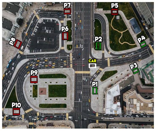
Figure 2. A real life parking spot choice problem.

Let $\mathcal{U}$ be a plithogenic universe of discourse consisting of all parking spots in the surrounding area, where

$$\mathcal{U}=\{P_1,P_2,P_3,\dots ,P_{10}\}.$$

The attributes of the parking spots, chosen for the decision, are $a_1,a_2,a_3,a_4$ given below:

$a_1$ = Parking fee,

$a_2$ = Distance between car and parking spot,

$a_3$ = Number of traffic signals between car and parking spot,

$a_4$ = Traffic density on the way between car and parking spot.

The attribute values of $a_1,a_2,a_3,a_4$ belong to the sets $A_1,A_2,A_3,A_4$, respectively.

$A_1=\{$ low fee ($f_1$), medium fee ($f_2$), high fee ($f_3$)},

$A_2=\{$ very near ($r_1$), almost near ($r_2$), near ($r_3$), almost far ($r_4$), far ($r_5$), very far ($r_6\left)\right\}$,

$A_3=\{$ one signal ($s_1$), two signals ($s_2\left)\right\}$,

$A_4=\{$ low ($d_1$), high ($d_2$), very high ($d_3\left)\right\}$.

The dominant attribute values of $a_1,a_2,a_3,a_4$ are chosen to be $f_1,r_1,s_1$ and $d_1$, respectively, and the single-valued fuzzy degree of contradiction between the dominant attribute value and all other attribute values is given below.

$$\begin{array}{c}\hfill \begin{array}{cc}& c_F(f_1,f_2)=\frac{1}{3},c_F(f_1,f_3)=\frac{2}{3},\hfill \\ & c_F(r_1,r_2)=\frac{1}{6},c_F(r_1,r_3)=\frac{2}{6},c_F(r_1,r_4)=\frac{3}{6},c_F(r_1,r_5)=\frac{4}{6},c_F(r_1,r_6)=\frac{5}{6},\hfill \\ & c_F(s_1,s_2)=\frac{1}{2},\hfill \\ & c_F(d_1,d_2)=\frac{1}{3},c_F(d_1,d_3)=\frac{2}{3}.\hfill \end{array}\end{array}$$

Two different sets of alternatives are considered for the application of PHSS-based TOPSIS, along with a comparison with fuzzy TOPSIS in each case.

4.2.1. Case 1

In this case, the parking spots under consideration (alternatives) are contained in the set $X\subseteq \mathcal{U}$, given by

$$X=\{P_1,P_2,P_3,P_4\}.$$

The neutrosophic degree of appurtenance of each attribute value corresponding to each alternative $P_1,P_2,P_3,P_4$ is given in Table 1.

Table 1. Degree of appurtenance of each attribute value w.r.t. to each alternative.

Sr.	Variables	${\mathit{P}}_1$	${\mathit{P}}_2$	${\mathit{P}}_3$	${\mathit{P}}_4$
1	$f_1$	(0.5, 0.1, 0.3)	(0.5, 0.0, 0.7)	(0.1, 0.4, 0.5)	(0.2, 0.1, 0.6)
2	$f_2$	(0.7, 0.9, 0.1)	(0.6, 0.5, 0.2)	(0.2, 0.3, 0.6)	(0.7, 0.9, 0.3)
3	$f_3$	(0.5, 0.5, 0.1)	(0.0, 0.1, 0.5)	(0.1, 0.1, 0.9)	(0.5, 0.7, 0.2)
4	$r_1$	(0.8, 0.1, 0.7)	(0.9, 0.4, 0.5)	(0.9, 0.4, 0.0)	(0.8, 0.4, 0.2)
5	$r_2$	(0.9, 0.3, 0.2)	(0.6, 0.1, 0.0)	(0.5, 0.2, 0.4)	(0.9, 0.1, 0.4)
6	$r_3$	(0.9, 0.1, 0.3)	(0.8, 0.3, 0.1)	(0.6, 0.0, 0.6)	(0.2, 0.2, 0.5)
7	$r_4$	(0.8, 0.3, 0.2)	(1.0, 0.1, 0.5)	(0.8, 0.5, 0.1)	(0.7, 0.3, 0.6)
8	$r_5$	(1.0, 0.3, 0.2)	(1.0, 0.3, 0.2)	(0.8, 0.2, 0.8)	(0.6, 0.5, 0.6)
9	$r_6$	(0.8, 0.1, 0.0)	(0.6, 0.8, 0.5)	(0.9, 0.7, 0.1)	(0.4, 0.8, 0.7)
10	$s_1$	(0.0, 0.5, 0.5)	(0.4, 0.1, 0.6)	(0.2, 0.2, 0.7)	(0.8, 0.3, 0.4)
11	$s_2$	(1.0, 0.8, 0.6)	(0.7, 0.5, 0.5)	(0.4, 0.4, 0.7)	(0.6, 0.5, 0.7)
12	$d_1$	(0.1, 0.2, 1.0)	(0.3, 1.0, 0.6)	(0.7, 0.9, 0.2)	(0.9, 0.7, 0.5)
13	$d_2$	(0.1, 0.4, 0.8)	(0.2, 0.2, 0.8)	(0.2, 0.6, 0.3)	(0.2, 0.8, 0.5)
14	$d_3$	(0.5, 0.6, 0.9)	(0.9, 0.6, 0.3)	(0.9, 0.7, 0.5)	(0.6, 0.7, 0.6)

Let $C=A_1\times A_2\times A_3\times A_4$ and consider an element $(f_2,r_1,s_2,d_1)\in C$ for which the corresponding matrix that was obtained from Table 1 is given below:

$$\begin{array}{c}\hfill \left[\begin{array}{cccc}(0.7,0.9,0.1)& (0.6,0.5,0.2)& (0.2,0.3,0.6)& (0.7,0.9,0.3)\\ (0.8,0.1,0.7)& (0.9,0.4,0.5)& (0.9,0.4,0.0)& (0.8,0.4,0.2)\\ (1.0,0.8,0.6)& (0.7,0.5,0.5)& (0.4,0.4,0.7)& (0.6,0.5,0.7)\\ (0.1,0.2,1.0)& (0.3,1.0,0.6)& (0.7,0.9,0.2)& (0.9,0.7,0.5)\end{array}\right]\end{array}$$

(2)

This MCDM problem is solved by the proposed PHSS-based TOPSIS and fuzzy TOPSIS, as follows:

A. Application of PHSS-based TOPSIS for Case 1

Apply the plithogenic accuracy function (1) to the matrix (2) in order to obtain the plithogenic accuracy matrix given by:

$$\begin{array}{c}\hfill \left[\begin{array}{cccc}0.6667& 0.5667& 0.4778& 0.7333\\ 0.5333& 0.6000& 0.4333& 0.4667\\ 0.9667& 0.7500& 0.6833& 0.8500\\ 0.4333& 0.6333& 0.6000& 0.7000\end{array}\right].\end{array}$$

The plithogenic decision matrix $M_p$ is constructed by taking the transpose of the plithogenic accuracy matrix. It is a square matrix of order 4, given by

$$\begin{array}{c}\hfill M_p=\left[\begin{array}{cccc}0.6667& 0.5333& 0.9667& 0.4333\\ 0.5667& 0.6000& 0.7500& 0.6333\\ 0.4778& 0.4333& 0.6833& 0.6000\\ 0.7333& 0.4667& 0.8500& 0.7000\end{array}\right]\end{array}$$

A corresponding table, as shown in Table 2, of alternatives versus criteria may also be drawn to see the situation in a clear way.

Table 2. Alternatives versus criteria table.

$\mathit{Al}/\mathit{Cr}$	${\mathit{f}}_2$	${\mathit{r}}_1$	${\mathit{s}}_2$	${\mathit{d}}_1$
$P_1$	0.6667	0.5333	0.9667	0.4333
$P_2$	0.5667	0.6000	0.7500	0.6333
$P_3$	0.4778	0.4333	0.6833	0.6000
$P_4$	0.7333	0.4667	0.8500	0.7000

A plithogenic normalized decision matrix $N_p$ is obtained as:

$$\begin{array}{c}\hfill N_p=\left[\begin{array}{cccc}0.5387& 0.5205& 0.5898& 0.3612\\ 0.4579& 0.5855& 0.4576& 0.5280\\ 0.3861& 0.4229& 0.4169& 0.5002\\ 0.5925& 0.4555& 0.5186& 0.5836\end{array}\right]\end{array}$$

A weighted normalized matrix $W_4$ is constructed as:

$$W_4=[0.4,0.22,0.15,0.23],$$

(3)

whereas the plithogenic weighted normalized decision matrix $V_p={\left[v_{ij}\right]}_{4\times 4}$ is given, as follows:

$$\begin{array}{c}\hfill V_p=\left[\begin{array}{cccc}0.2155& 0.1145& 0.0885& 0.0831\\ 0.1832& 0.1288& 0.0686& 0.1214\\ 0.1544& 0.0930& 0.0625& 0.1150\\ 0.2370& 0.1002& 0.0778& 0.1342\end{array}\right]\end{array}$$

The plithogenic positive ideal solution $V_p^{+}$ and plithogenic negative ideal solution $V_p^{-}$ are determined, as follows:

$$\begin{array}{c}\hfill \begin{array}{cc}& V_p^{+}=\{0.1544,0.0930,0.0625,0.0831\},\hfill \\ & V_p^{-}=\{0.2370,0.1288,0.0885,0.1342\}.\hfill \end{array}\end{array}$$

The plithogenic distance of each alternative from the $V_p^{+}$ and $V_p^{-}$, respectively, is determined as:

$$\begin{array}{cc}\hfill & S^{+}=\left[\begin{array}{c}0.0697\\ 0.0601\\ 0.0320\\ 0.0986\end{array}\right],S^{-}=\left[\begin{array}{c}0.0573\\ 0.0588\\ 0.0956\\ 0.0305\end{array}\right].\hfill \end{array}$$

The relative closeness coefficient $C_i,i=1,2,3,4$, of each alternative is computed as:

$$\begin{array}{cc}\hfill & C_1=0.4511,\hfill \\ & C_2=0.4944,\hfill \\ & C_3=0.7494,\hfill \\ & C_4=0.2366.\hfill \end{array}$$

The highest value corresponds to the most suitable alternative. Since $C_3=0.7494$ is the maximum value and it corresponds to $P_3$, therefore, the most suitable parking spot is $P_3$. The Table 3 is constructed to rank all alternatives under consideration.

Table 3. PHSS-based TOPSIS ranking table.

	${\mathit{S}}_{\mathit{i}}^{+}$	${\mathit{S}}_{\mathit{i}}^{-}$	${\mathit{C}}_{\mathit{i}}$	Ranking
$P_1$	0.0697	0.0573	0.4511	3
$P_2$	0.0601	0.0588	0.4944	2
$P_3$	0.0320	0.0956	0.7494	1
$P_4$	0.0986	0.0305	0.2366	4

A bar graph presented in Figure 3 is given, in which all alternatives $P_1,P_2,P_3,P_4$ are ranked by PHSS-based TOPSIS.

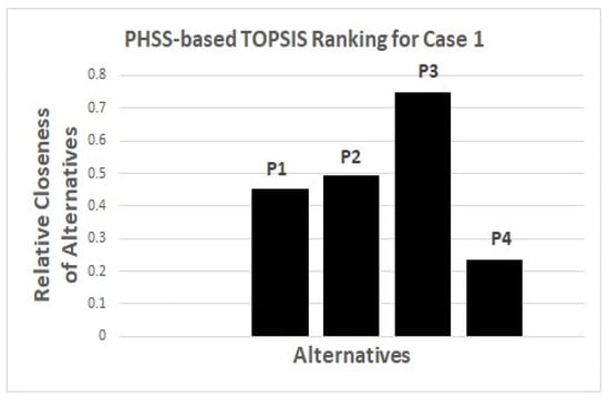
Figure 3. Ranking of Parking Spots by PHSS-based TOPSIS for Case 1.

It is evident that the parking spot $P_3$ is the most suitable place to park the car while $P_4$ is not a good choice for parking based on the selection criteria.

B. Application of Fuzzy TOPSIS for Case 1

In order to see the implementation of fuzzy TOPSIS [32,33,34] for the current scenario of the parking problem, we apply the average operator [27,35] to each element of the matrix 2 and take the transpose of the resulting matrix in order to obtain the decision matrix given by:

$$\begin{array}{c}\hfill M=\left[\begin{array}{cccc}0.5667& 0.5333& 0.8000& 0.4333\\ 0.4333& 0.6000& 0.5667& 0.6333\\ 0.3667& 0.4333& 0.5000& 0.6000\\ 0.6333& 0.4667& 0.6000& 0.7000\end{array}\right]\end{array}$$

Applying the fuzzy TOPSIS to the decision matrix M, along with the same weights given in matrix (3), we obtain the values of positive distance $S^{+}$, negative distance $S^{-}$, relative closeness $C_i$ and ranking of each alternative, as given in Table 4.

Table 4. Fuzzy TOPSIS ranking table.

	${\mathit{S}}_{\mathit{i}}^{+}$	${\mathit{S}}_{\mathit{i}}^{-}$	${\mathit{C}}_{\mathit{i}}$	Ranking
$P_1$	0.0888	0.0592	0.4000	3
$P_2$	0.0591	0.0841	0.5872	2
$P_3$	0.0320	0.1176	0.7863	1
$P_4$	0.1170	0.0373	0.2417	4

A bar graph in Figure 4 is given in which all alternatives $P_1,P_2,P_3,P_4$ are ranked by Fuzzy TOPSIS.

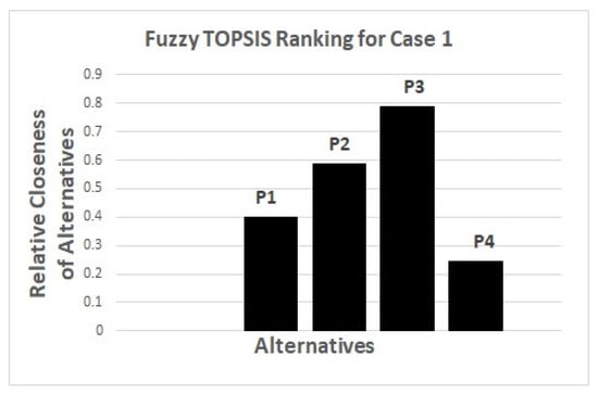
Figure 4. Ranking of Parking Spots by Fuzzy TOPSIS for Case 1.

A comparison is shown in Table 5, in which it can be seen that the result obtained by the proposed PHSS-based TOPSIS is aligned with that of fuzzy TOPSIS.

Table 5. Comparison analysis for case 1.

Sr.	Parkings	PHSS-Based TOPSIS Ranking	Fuzzy TOPSIS Ranking
1	$P_1$	3rd	3rd
2	$P_2$	2nd	2nd
3	$P_3$	1st	1st
4	$P_4$	4th	4th

It is observed in Table 5 that the results obtained by both methods coincide in terms of the ranking of each alternative, but differ in the values of the relative closeness of each alternative. It is due to the nature of the MCDM problem in hand in which each alternative needs to be evaluated against each attribute value possessing a neutrosophic degree of appurtenance w.r.t. each alternative and a contradiction degree is defined between each attribute value and its corresponding dominant attribute value to be taken into consideration in the decision process. In such a case, the proposed PHSS-based TOPSIS produces a more reliable relative closeness of each alternative, as it can been seen in the parking spot choice problem that was chosen for the study. Therefore, it is worth noting that the proposed PHSS-based TOPSIS can be regarded as a generalization of fuzzy TOPSIS [32], because the fuzzy TOPSIS cannot be directly applied to MCDM problems in which the attribute values have a neutrosophic degree of appurtenance with respect to each alternative. In the case of the parking problem, fuzzy TOPSIS is applied after applying simple average operator to the neutrosophic elements of the matrix (2). However, it does not takes into account the degree of contradiction between the attribute values, which is the limitation of fuzzy TOPSIS. This concern is precisely addressed by the proposed PHSS-based TOPSIS.

4.2.2. Case 2

In this case, the set of parking spots under consideration is given by

$$X=\{P_1,P_5,P_6,P_7\}.$$

The neutrosophic degree of appurtenance of each attribute value that corresponds to each alternative of $\{P_1,P_5,P_6,P_7\}$ is given in Table 6.

Table 6. Degree of appurtenance of each attribute value w.r.t each alternative.

Sr.	Variables	${\mathit{P}}_1$	${\mathit{P}}_5$	${\mathit{P}}_6$	${\mathit{P}}_7$
1	$f_1$	(0.5, 0.1, 0.3)	(0.6, 0.6, 0.8)	(0.7, 0.2, 0.4)	(0.9, 0.5, 0.2)
2	$f_2$	(0.7, 0.9, 0.1)	(0.8, 0.8, 0.5)	(0.4, 0.4, 0.7)	(0.7, 0.2, 0.1)
3	$f_3$	(0.5, 0.5, 0.1)	(0.4, 0.2, 0.5)	(1.0, 0.5, 0.9)	(1.0, 0.7, 0.6)
4	$r_1$	(0.8, 0.1, 0.7)	(0.9, 0.5, 0.2)	(0.5, 0, 0.9)	(0.8, 0.6, 0.1)
5	$r_2$	(0.9, 0.3, 0.2)	(0.5, 0.4, 0.2)	(0.7, 0.5, 0.4)	(0.9, 0.6, 0.8)
6	$r_3$	(0.9, 0.1, 0.3)	(0.5, 0.7, 0.3)	(0.9, 1.0, 0.6)	(0.2, 0, 1.0)
7	$r_4$	(0.8, 0.3, 0.2)	(1.0, 0.2, 1.0)	(1.0, 0.5, 0.7)	(0.8, 0.8, 0.9)
8	$r_5$	(0.2, 0.3, 0.9)	(1.0, 0.1, 0.8)	(0.4, 0.6, 0.8)	(0.8, 0.6, 0.6)
9	$r_6$	(0.5, 0.7, 0.5)	(0.8, 0.2, 0.0)	(0.6, 0.3, 0.7)	(0.0, 0.9, 0.9)
10	$s_1$	(0, 0.5, 0.5)	(0.8, 0.4, 0.6)	(0.9, 0.2, 0.2)	(0.8, 0.4, 0.7)
11	$s_2$	(1.0, 0.8, 0.6)	(0.7, 1.0, 0.2)	(0.2, 0.4, 0.7)	(0.9, 0, 1.0)
12	$d_1$	(0.1, 0.2, 1.0)	(1.0, 0.4, 0.3)	(0.7, 0.5, 0.6)	(0.8, 0.5, 0.7)
13	$d_2$	(0.1, 0.4, 0.8)	(0.7, 1.0, 0.8)	(0.6, 0.6, 1.0)	(1.0, 0.8, 0.8)
14	$d_3$	(0.5, 0.6, 0.9)	(1.0, 0.6, 0.5)	(1.0, 1.0, 0.5)	(1.0, 0.5, 0.8)

Let $C=A_1\times A_2\times A_3\times A_4$ and consider an element $(f_2,r_1,s_2,d_1)\in C$ for which the corresponding matrix obtained from Table 6, is given below:

$$\begin{array}{c}\hfill \left[\begin{array}{cccc}(0.7,0.9,0.1)& (0.8,0.8,0.5)& (0.4,0.4,0.7)& (0.7,0.2,0.1)\\ (0.8,0.1,0.7)& (0.9,0.5,0.2)& (0.5,0.0,0.9)& (0.8,0.6,0.1)\\ (1.0,0.8,0.6)& (0.7,1.0,0.2)& (0.2,1.0,0.7)& (0.9,0.0,1.0)\\ (0.1,0.2,1.0)& (1.0,0.4,0.3)& (0.7,0.5,0.6)& (0.8,0.5,0.7)\end{array}\right]\end{array}$$

(4)

The proposed PHSS-based TOPSIS and fuzzy TOPSIS are employed, as follows:

A. Application of PHSS-Based TOPSIS for Case 2

The plithogenic accuracy matrix in this case is given by

$$\begin{array}{c}\hfill \left[\begin{array}{cccc}0.6667& 0.9222& 0.6444& 0.5111\\ 0.5333& 0.6000& 0.4333& 0.4667\\ 0.9667& 0.9333& 0.6500& 0.9500\\ 0.4333& 0.6333& 0.6000& 0.7000\end{array}\right].\end{array}$$

Plithogenic decision matrix $M_p$ is given by

$$\begin{array}{c}\hfill M_p=\left[\begin{array}{cccc}0.6667& 0.5333& 0.9667& 0.4333\\ 0.9222& 0.6000& 0.9333& 0.6333\\ 0.6444& 0.4333& 0.6500& 0.6000\\ 0.5111& 0.4667& 0.9500& 0.7000\end{array}\right]\end{array}$$

A plithogenic normalized decision matrix $N_p$ is then constructed as:

$$\begin{array}{c}\hfill N_p=\left[\begin{array}{cccc}0.4748& 0.5205& 0.5464& 0.3612\\ 0.6568& 0.5855& 0.5275& 0.5280\\ 0.4590& 0.4229& 0.3674& 0.5002\\ 0.3640& 0.4555& 0.5369& 0.5836\end{array}\right]\end{array}$$

The plithogenic weighted normalized decision matrix $V_p$ is given, as follows:

$$\begin{array}{c}\hfill V_p=\left[\begin{array}{cccc}0.1899& 0.1145& 0.0820& 0.0831\\ 0.2627& 0.1288& 0.0791& 0.1214\\ 0.1836& 0.0930& 0.0551& 0.1150\\ 0.1456& 0.1002& 0.0805& 0.1342\end{array}\right]\end{array}$$

The plithogenic positive ideal solution $V_p^{+}$ and plithogenic negative ideal solution $V_p^{-}$ are determined, such that

$$\begin{array}{c}\hfill \begin{array}{cc}& V_p^{+}=\{0.1456,0.0930,0.0551,0.0831\},\hfill \\ & V_p^{-}=\{0.2627,0.1288,0.0820,0.1342\}.\hfill \end{array}\end{array}$$

The plithogenic positive distance $S^{+}$, plithogenic negative distance $S^{-}$, relative closeness $C_i$, and ranking of each alternative is shown in Table 7.

Table 7. PHSS-based TOPSIS ranking table.

	${\mathit{S}}_{\mathit{i}}^{+}$	${\mathit{S}}_{\mathit{i}}^{-}$	${\mathit{C}}_{\mathit{i}}$	Ranking
$P_1$	0.0561	0.0901	0.6163	3
$P_5$	0.1306	0.0131	0.0912	4
$P_6$	0.0496	0.0929	0.6518	2
$P_7$	0.0576	0.1206	0.6769	1

A graphical representation of the ranking of all alternatives obtained by PHSS-based TOPSIS, is shown in Figure 5.

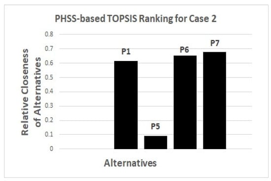
Figure 5. Ranking of Parking Spots by PHSS-based TOPSIS for Case 2.

It can be seen that the parking spot $P_7$ is the most suitable alternative in the light of chosen criteria.

B. Application of Fuzzy TOPSIS for Case 2

In this case, the decision matrix M for the implementation of fuzzy TOPSIS is given by

$$\begin{array}{c}\hfill M=\left[\begin{array}{cccc}0.5667& 0.5333& 0.8000& 0.4333\\ 0.7000& 0.6000& 0.6333& 0.6333\\ 0.5000& 0.4333& 0.6333& 0.6000\\ 0.3333& 0.4667& 0.6333& 0.7000\end{array}\right]\end{array}$$

By implementing the fuzzy TOPSIS to the matrix M, with the same weights given in (3), the values of positive distance $S^{+}$, negative distance $S^{-}$, relative closeness $C_i$, and ranking of each alternative are shown in Table 8.

Table 8. Fuzzy TOPSIS ranking table.

	${\mathit{S}}_{\mathit{i}}^{+}$	${\mathit{S}}_{\mathit{i}}^{-}$	${\mathit{C}}_{\mathit{i}}$	Ranking
$P_1$	0.0908	0.0724	0.4439	3
$P_5$	0.1453	0.0224	0.1337	4
$P_6$	0.0694	0.0863	0.5543	2
$P_7$	0.0516	0.1397	0.7301	1

The ranking of all alternatives can also been visualized as a bar graph in Figure 6, in which all alternatives $P_1,P_5,P_6,P_7$ are ranked by Fuzzy TOPSIS.

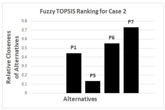
Figure 6. Ranking of Parking Spots by Fuzzy TOPSIS for Case 2.

The most suitable parking spot obtained by fuzzy TOPSIS is also $P_7$.

A comparison of rankings obtained by PHSS-based TOPSIS and fuzzy TOPSIS is shown in Table 9 for case 2.

Table 9. Comparison analysis for case 2.

Sr.	Parkings	PHSS-Based TOPSIS Ranking	Fuzzy TOPSIS Ranking
1	$P_1$	3rd	3rd
2	$P_5$	4th	4th
3	$P_6$	2nd	2nd
4	$P_7$	1st	1st

It may be noted that similar results are obtained in case 2, with the help of proposed PHSS-based TOPSIS and fuzzy TOPSIS with exactly same ranking of each alternative, but with a considerably different values of the relative closeness of each alternative as shown in Table 9. Therefore, it is accomplished that the results that were obtained by the PHSS-based TOPSIS are valid and more reliable and PHSS-based TOPSIS can be regarded as the generalization of fuzzy TOPSIS on the basis of the study conducted in the article.

5. Conclusions

It has always been a challenging task to deal with real life MCDM problems, due to the involvement of many complexities and uncertainties. In particular, some real life MCDM problems are designed in a way that the given attributes need to be further decomposed into two or more attribute values such that each alternative is then required to be evaluated against each attribute value in order to perform a detailed analysis to reach a fair conclusion. To deal with such situations, a novel PHSS-based TOPSIS is proposed in the present study, and it is applied to a MCDM parking problem with different choices of the set of alternatives and a comparison with fuzzy TOPSIS is done to prove the validity and efficiency of the proposed method. All of the results are quite promising and graphically depicted for a clear understanding. Moreover, the algorithm of the proposed method is produced in MATLAB in order to broaden the scope of the study to other research areas, including graph theory, machine learning, pattern recognition, etc.

References

- Zadeh, L.A. Fuzzy sets. Inform. Control 1965, 8, 338–353. [Google Scholar] [CrossRef]
- Yang, M.S.; Hung, W.L.; Chang-Chien, S.J. On a similarity measure between LR-type fuzzy numbers and its application to database acquisition. Int. J. Intell. Syst. 2005, 20, 1001–1016. [Google Scholar] [CrossRef]
- Meng, F.; Tang, J.; Fujita, H. Consistency-based algorithms for decision-making with interval fuzzy preference relations. IEEE Trans. Fuzzy Syst. 2019, 27, 2052–2066. [Google Scholar] [CrossRef]
- Ruiz-Garca, G.; Hagras, H.; Pomares, H.; Ruiz, I.R. Toward a fuzzy logic system based on general forms of interval type-2 fuzzy sets. IEEE Trans. Fuzzy Syst. 2019, 27, 2381–2395. [Google Scholar] [CrossRef]
- Ullah, K.; Hassan, N.; Mahmood, T.; Jan, N.; Hassan, M. Evaluation of investment policy based on multi-attribute decision-making using interval valued T-spherical fuzzy aggregation operators. Symmetry 2019, 11, 357. [Google Scholar] [CrossRef]
- Atanassov, K.T. Intuitionistic fuzzy sets. Fuzzy Sets Syst. 1986, 20, 87–96. [Google Scholar] [CrossRef]
- Hwang, C.M.; Yang, M.S.; Hung, W.L. New similarity measures of intuitionistic fuzzy sets based on the Jaccard index with its application to clustering. Int. J. Intell. Syst. 2018, 33, 1672–1688. [Google Scholar] [CrossRef]
- Garg, H.; Kumar, K. Linguistic interval-valued atanassov intuitionistic fuzzy sets and their applications to group decision making problems. IEEE Trans. Fuzzy Syst. 2019, 27, 2302–2311. [Google Scholar] [CrossRef]
- Roy, J.; Das, S.; Kar, S.; Pamucar, D. An extension of the CODAS approach using interval-valued intuitionistic fuzzy set for sustainable material selection in construction projects with incomplete weight information. Symmetry 2019, 11, 393. [Google Scholar] [CrossRef]
- Yang, M.S.; Hussian, Z.; Ali, M. Belief and plausibility measures on intuitionistic fuzzy sets with construction of belief-plausibility TOPSIS. Complexity 2020, 1–12. [Google Scholar] [CrossRef]
- Smarandache, F. A Unifying Field in Logics: Neutrosophic Logic. Neutrosophy, Neutrosophic Set, Probability, and Statistics, 2nd ed.; American Research Press: Rehoboth, DE, USA, 2000. [Google Scholar]
- Majumdar, P.; Samanta, S.K. On similarity and entropy of neutrosophic sets. J. Intell. Fuzzy Syst. 2014, 26, 1245–1252. [Google Scholar] [CrossRef]
- Li, X.; Zhang, X.; Park, C. Generalized interval neutrosophic Choquet aggregation operators and their applications. Symmetry 2018, 10, 85. [Google Scholar] [CrossRef]
- Abdel-Basset, M.; Mohamed, M. A novel and powerful framework based on neutrosophic sets to aid patients with cancer. Future Gener. Comput. Syst. 2019, 98, 144–153. [Google Scholar] [CrossRef]
- Vasantha, W.B.; Kandasamy, I.; Smarandache, F. Neutrosophic components semigroups and multiset neutrosophic components semigroups. Symmetry 2020, 12, 818. [Google Scholar]
- Molodtsov, D. Soft set theory-first results. Comput. Math. Appl. 1999, 37, 19–31. [Google Scholar] [CrossRef]
- Maji, P.K.; Biswas, R.; Roy, A.R. Soft set theory. Comput. Math. Appl. 2003, 45, 555–562. [Google Scholar] [CrossRef]
- Ali, M.I.; Feng, F.; Liu, X.; Min, W.K.; Shabir, M. On some new operations in soft set theory. Comput. Math. Appl. 2009, 57, 1547–1553. [Google Scholar] [CrossRef]
- Inthumathi, V.; Chitra, V.; Jayasree, S. The role of operators on soft sets in decision making problems. Int. J. Comput. Appl. Math. 2017, 12, 899–910. [Google Scholar]
- Feng, G.; Guo, X. A novel approach to fuzzy soft set-based group decision-making. Complexity 2018, 2018, 2501489. [Google Scholar] [CrossRef]
- Biswas, B.; Bhattacharyya, S.; Chakrabarti, A.; Dey, K.N.; Platos, J.; Snasel, V. Colonoscopy contrast-enhanced by intuitionistic fuzzy soft sets for polyp cancer localization. Appl. Soft Comput. 2020, 95, 106492. [Google Scholar] [CrossRef]
- Smarandache, F. Extension of soft set to hypersoft set, and then to plithogenic hypersoft set. Neutrosophic Sets Syst. 2018, 22, 168–170. [Google Scholar]
- Saeed, M.; Ahsan, M.; Siddique, M.K.; Ahmad, M.R. A study of the fundamentals of hypersoft set theory. Int. Sci. Eng. Res. 2020, 11, 320–329. [Google Scholar]
- Smarandache, F. Plithogeny, Plithogenic Set, Logic, Probobility, and Statistics; Pons: Brussels, Belgium, 2017. [Google Scholar]
- Smarandache, F. Plithogenic set, an extension of crisp, fuzzy, intuitionistic fuzzy, and neutrosophic sets-revisited. Neutrosophic Sets Syst. 2018, 21, 153–166. [Google Scholar]
- Collan, M.; Luukka, P. Evaluating R & D projects as investments by using an overall ranking from four new fuzzy similarity measure-based TOPSIS variants. IEEE Trans. Fuzzy Syst. 2014, 22, 505–515. [Google Scholar]
- Saqlain, M.; Saeed, M.; Ahmad, M.R.; Smarandache, F. Generalization of TOPSIS for neutrosophic hypersoft set using accuracy function and its application. Neutrosophic Sets Syst. 2019, 27, 131–137. [Google Scholar]
- Khalil, A.M.; Cao, D.; Azzam, A.; Smarandache, F.; Alharbi, W.R. Combination of the single-valued neutrosophic fuzzy set and the soft set with applications in decision-making. Symmetry 2020, 12, 1361. [Google Scholar] [CrossRef]
- Abdel-Basset, M.; Mohamed, R. A novel plithogenic TOPSIS-CRITIC model for sustainable supply chain risk management. J. Clean. Prod. 2020, 247, 119586. [Google Scholar] [CrossRef]
- Schumann, A. p-Adic valued logical calculi in simulation of the slime mould behaviour. J. Appl. Non-Class. Logics 2015, 25, 125–139. [Google Scholar] [CrossRef]
- Schumann, A. p-Adic multiple-validity and p-adic valued logical calculi. J. Mult.-Valued Log. Soft Comput. 2007, 13, 29–60. [Google Scholar]
- Yang, T.; Hung, C.C. Multiple-attribute decision making methods for plant layout design problem. Robot. Comput.-Integr. 2007, 23, 126–137. [Google Scholar] [CrossRef]
- Kabir, G.; Hasin, M. Comparative analysis of topsis and fuzzy topsis for the evaluation of travel website service quality. Int. Qual. Res. 2012, 6, 169–185. [Google Scholar]
- Zhang, L.; Zhan, J.; Yao, Y. Intuitionistic fuzzy TOPSIS method based on CVPIFRS models: An application to biomedical problems. Inf. Sci. 2020, 517, 315–339. [Google Scholar] [CrossRef]
- Yager, R.R. The power average operator. IEEE Trans. Syst. Man Cybern. Syst. Hum. 2001, 31, 724–731. [Google Scholar] [CrossRef]
Publisher’s Note: MDPI stays neutral with regard to jurisdictional claims in published maps and institutional affiliations. |
© 2020 by the authors. Licensee MDPI, Basel, Switzerland. This article is an open access article distributed under the terms and conditions of the Creative Commons Attribution (CC BY) license (http://creativecommons.org/licenses/by/4.0/).