Analogy between Thermodynamic Phase Transitions and Creeping Flows in Rectangular Cavities


Department of Physics, Cleveland State University, 2121 Euclid Avenue, Cleveland, OH 44115, USA
*
Author to whom correspondence should be addressed.
Symmetry 2020, 12(11), 1859; https://doi.org/10.3390/sym12111859
Submission received: 9 October 2020
/
Revised: 27 October 2020
/
Accepted: 7 November 2020
/
Published: 12 November 2020
(This article belongs to the Special Issue Symmetry and Symmetry Breaking: Phase Transitions and Critical Phenomena)
Abstract
:An analogy is found between the streamline function corresponding to Stokes flows in rectangular cavities and the thermodynamics of phase transitions and critical points. In a rectangular cavity flow, with no-slip boundary conditions at the walls, the corners are fixed points. The corners defined by a stationary and a moving wall, are found to be analogous to a thermodynamic first-order transition point. In contrast, the corners defined by two stationary walls correspond to thermodynamic critical points. Here, flow structures, also known as Moffatt eddies, form and act as stagnation regions where mixing is impeded. A third stationary point occurs in the middle region of the channel and it is analogous to a high temperature thermodynamic fixed point. The numerical results of the fluid flow modeling are correlated with analytical work in the proximity of the fixed points.
PACS Classification:
47.15.G-; 64.60.Ak; 64.60.ae1. Introduction
The characterization of fluid flows in rectangular domains is a fundamental problem in fluid dynamics with applications to: cavity flow [1], polymer melt flow in extruders [2], and microfluidics [3,4]. Those physical systems are characterized by small Reynolds numbers. This is why we focus our attention on creeping flows (zero Reynolds number). In this paper, we point to an analogy between the fluid mechanics problem and the thermodynamic critical phenomena and phase transitions problem. Close to the corners, the streamline function, the velocity field and the pressure exhibit power law behavior [5,6,7] as a function of the distance to the corner, not unlike the power law dependence of various thermodynamic quantities (free energy, energy, heat capacity) as a function of the reduced temperature (distance to the critical point). Analogies between fluid mechanics problems and critical thermodynamic phenomena, under the common roof of complex phenomena, were presented by Goldenfeld and Kadanoff [8]. At the corner where the adjacent walls are stationary, we find self-similar structures, also known as Moffatt [5,6] eddies. These structures are important in the design of polymer extruders and microchannels systems, as their presence negatively impacts the ability to achieve uniform mixing [9]. This phenomenon is analogous to the log-periodicity [10] of the critical amplitude of the free energy close to critical points on hierarchical lattices [11,12,13]. The corner of the rectangular cavity, with one adjacent moving wall and the other adjacent wall stationary, is analogous to a first-order thermodynamic transition [14]. The velocity varies between the moving wall velocity and zero, at the stationary wall. The thermodynamic analog is as follows: for Ising-like ferromagnetic transitions at low temperatures, the magnetization changes from +1 to −1 as the magnetic field changes sign. To complete the list of analogies, the stationary point in the central region of the cavity resembles a high temperature paramagnetic point in the Ising model.
The remainder of this paper contains: a qualitative description of the renormalization group solution of critical thermodynamic phenomena and phase transitions in Section 2, a description of the numerical techniques used to solve the Navier–Stokes equations in Section 3, the power law solutions to the Navier–Stokes equations in Section 4, the critical point analog in Section 5, the discontinuity point analog in Section 6, and the high temperature point analog in Section 7.
A summary of our findings is contained in Section 8.
2. Renormalization Group Theory of Critical Phenomena and Phase Transitions
The fundamental quantity of statistical mechanics [15] is the partition function. Its logarithm provides the free energy f. In the renormalization method, one sums a fraction of the variables thus obtaining a restricted partition function depending on the un-summed variables.
This process is repeated until all degrees of freedom are summed up. A sequence of effective Hamiltonians is generated. The Hamiltonians flow to a fixed-point Hamiltonian. The stability of the renormalization group flow at the fixed point determines the critical exponents. In simple Ising-like problems, one gets three types of fixed points. At T = 0, there is the discontinuity fixed point [14] that governs the coexisting phases. It describes the first order transition of the symmetry-breaking type between ferromagnetic phases. At T = TC, one gets a critical fixed point. Close to the critical point [16], one gets a power law dependence of the free energy: f~|t|2−α, where t measures the distance to the critical temperature. Finally, at T = ∞, there is a stable fixed point governing the paramagnetic phase. From this type of analysis, the power laws for the thermodynamic quantities are derived. Criticality is universal [8] as the exponents are found to depend only on a few characteristics of the system such as symmetry, range of interactions and spatial dimension.
3. Numerical Modeling
The fluid flow in this work has been modeled using the software package COMSOL Multiphysics and its Computational Fluid Dynamics/Chemical Engineering Module, under steady state flow conditions. The accuracy of the numerical work has been previously validated against well described cavity flows [1]. The solutions to the Navier–Stokes equations presented here are for an incompressible Newtonian fluid with density and viscosity corresponding to glycerine at room temperature, i.e., 1.261 × 10³ kg/m3 and 1410 × 10−3 kg/(m s), respectively. The height of the cavity is set to 2.5 cm and the width is adjusted from 2.5 to 12.5 cm to obtain aspect ratios (= width/height) from 1 to 5. These geometrical parameters correspond to those typically employed in the experimental study of rectangular cavity flows [17]. The top wall of the cavity is moving with speeds set in the range of 0.005–0.1 m/s, as described in the discussion section. Across the entire range of velocities used, the Reynolds number is small, corresponding to the Stokes flow regime. Non-slip boundary conditions are set for all the walls. The Navier–Stokes equations are solved using an iterative solver based on the generalized minimal residual method (GMRES). The Vanka algorithm setting is used for both the pre- and post-smoothing. Figure 1 shows typical numerical results for the flow fields in this type of cavities. The resolution of the numerical simulations used allows the observation of a hierarchical structure of up to three Moffatt eddies in the corner regions defined by two stationary walls.
4. Cavity Fluid Mechanics
Berker’s discovery [11] that the Migdal–Kadanoff renormalization-group scheme provides exact solutions of thermodynamic models on hierarchical lattices is important in view of the fact that it preserves the free energy convexity [18]. In [1], we emulated this approach in fluid mechanics by changing the boundary conditions to make the problem amenable to develop an analytical solution. In this paper, we consider the flow problem with the correct (no-slip) boundary conditions by using valid analytical methods close to the corners and numerical solutions.
We start with the steady state Navier–Stokes and continuity equations for the 2D case in which the inertial terms are neglected (zero Reynolds number):
where p stands for pressure, vx and vy are the velocity components and η is the viscosity.
Following from Equation (2), there exists a streamline function Ψ(x,y), such that the fluid velocities will be given by:
Substituting Equation (3) into Equation (1) we get:
Equation (4) implies:
Hence, the velocity is obtained from first-order derivatives while stresses, including pressure, are second-order derivatives of the streamline function with respect to coordinates. We consider non-slip boundary conditions. The top wall moves with constant velocity dragging the fluid. The other three walls are at rest.
Moffatt and Barenblatt [5,6,7] have demonstrated the relevance of self-similar solutions and power laws close to the corners.
The thermodynamic analogs of the streamline function, the velocity and the stress are the free energy which, close to the critical point, is f~|t|2−α, the energy U~|t|1−α, and the heat capacity C~|t|−α, respectively.
5. Critical Point Analog
At the corner where both adjacent walls are stationary, the exponent λ is a complex number:
λ = 1 + p + iq
This is an asymptotic relation valid in the limit of small r, the distance from the corner. The exponent was determined by Moffatt [5] in the limit of zero Reynolds number (creeping flow),
p = 2.74, q = 1.13
The fact that the exponent has an imaginary part manifests in the occurrence of an infinite sequence of eddies. Due to the real part of the exponent, the extent of the eddy quickly gets exponentially smaller as it approaches the corner. At the center of such an eddy, the velocity is zero. At the borders between adjacent eddies, the velocity has a local maximum. We solved numerically the Navier–Stokes equation for a finite, though small Reynolds number. The size of the region occupied by the individual eddies decreases exponentially as a function of the proximity to the corner. The resolution of the numerical modeling used allowed for the visualization of three eddies in the sequence. To verify the power laws, Equations (6) and (7), we looked at the maximum velocity in each period as a function of the distance to the cavity corner, see Figure 2.
The best fit yielded and exponent of p = 2.76 in good agreement with Moffatt’s value of p = 2.74. The distances from the centers of the Moffatt vortexes (where the velocity is null) to the corner form a sequence Rminn that scales a with a different exponent: Rminn. ω is determined by q, the imaginary part of λ. Moffatt’s theoretical value is: ω = π/q = 2.79. Numerically, we estimate ω = 2.82. There is a similar sequence Rmaxn distance from the points of maximum speed (border between adjacent eddies) to the corner. The numerical estimate is Rmaxn with ω = 2.79. In Figure 3, we show the Rmax and Rmin dependence on n for the three eddies that we have analyzed. Both ω estimates are in good agreement with Moffatt’s theoretical value.
We further analyzed the whole range of data from corner to center of cavity using a power law dependence. Within the field of critical thermodynamic phenomena, this approach has been pioneered by Riedel and Wegner [19] who developed the concept of the effective critical exponent. The data follow a power law quite precisely for more than 10 decades in velocity and for more than 4 decades in distance to corner, see Figure 4. We estimate an effective exponent peffective = 2.50. The quality of the fit ln(v)~peffective ln(r) is measured by the R-squared = 0.98.
These data were collected along a straight line from corner at an angle of 45 degrees with the horizontal. We have also looked at data along lines at angles of 22.5 degrees and 67.5 degrees. We notice a phenomenon akin to universality where the effective exponent is practically independent of the angle. Independence of the power law is observed also with respect to the varying velocity of the top wall and the aspect ratio of the channel, see Figure 5. Universality, and power laws, are central features [8] of critical phenomena and are also exhibited by the cavity flows.
6. Discontinuity Point Analog
At the corner where one wall is moving while the adjacent wall is stationary, the streamline function scales as: in the limit of small r, the distance from the corner. This was shown by Moffatt [6] for zero Reynolds number (creeping flow). Hence the exponent λ, see Equation (6), is:
λ = 1
This is the analog to Fisher and Berker [14] thermodynamic discontinuity fixed point requirement that the magnetic exponent equals the spatial dimension (yH/D = 1). This value of λ ensures that the velocity (i.e., the first derivative of stream function) is constant, V~r0 = constant, as the corner is approached, see Figure 6. The value of the constant depends on the angle of approach. The angle is zero along the moving wall and it is 90° along the fixed wall. Hence at fixed small r, as the angle is changed from zero to ninety degrees, the velocity varies from the moving wall velocity value to zero. Interestingly enough, the dependence is not monotonic.
7. High Temperature Point Analog
The stagnation point at the center of the cavity is an elliptical fixed point. It is similar to a high temperature fixed point in critical phenomena, in view of the analytical variation of the velocity as the point is approached. Since V~r1, see Figure 7, the exponent λ = 2.
8. Summary
We have presented an analogy between flows in rectangular cavities and thermodynamic phase transitions. For no-slip boundary conditions, the corners of the rectangular cavity are fixed points. The renormalization group theory of critical phenomena and phase transitions is based on fixed points. This is the base for the analogy. The corner with two adjacent stationary walls is analogous to a critical point. The Moffatt eddies emerge as a result of the imaginary part of the critical exponent. Its analog is the fact that critical amplitude on hierarchical lattice models is a log-periodic function. The corner with one adjacent moving wall and one stationary wall is analogous to a discontinuity (first-order transition) fixed point.
Beside the intrinsic interest in connecting apparently disparate fields of physics, this observation may have practical applications. Cavity flows, polymer melt flowing in extruders and flows in microchannels are approximated by flows in rectangular cavities. Our finding that scaling with an effective exponent holds quite well far from the corners can be used to get fast numerical estimates. This approach was suggested by the critical phenomena methodology usage of the effective exponent. We plan to further study what happens to the Moffatt eddies and to the critical exponents as the Reynolds number is increased. Do they vary continuously with the Reynolds number? Or do they stay unchanged until some threshold?
A thermodynamic critical point, in the Ising universality class, has a co-dimension [20] equal to two, as there are two relevant scaling fields: reduced temperature along the coexistence line and the magnetic field that breaks the symmetry between the coexisting ferromagnetic phases. In our fluid mechanics problem, we have identified only one such relevant scaling field: the distance to the corner. Further work is required to determine whether there is a second relevant field for the creeping flow problem studied here.
Author Contributions
Data curation, P.S.F.; formal analysis, M.K.; finite-element analysis, P.S.F.; writing—original draft, M.K. All authors have read and agreed to the published version of the manuscript.
Funding
This research received no external funding.
Conflicts of Interest
The authors declare no conflict of interest.
References
- Kaufman, M.; Fodor, P.S. Fluid mechanics in rectangular cavities—Analytical model and numerics. Phys. A Stat. Mech. Appl. 2010, 389, 2951–2955. [Google Scholar] [CrossRef]
- Tadmor, Z.; Gogos, G. Principles of Polymer Processing, 2nd ed.; John Wiley & Sons: Hoboken, NJ, USA, 2006. [Google Scholar]
- Squires, T.M.; Quake, S.R. Microfluidics: Fluid physics at the nanoliter scale. Rev. Mod. Phys. 2005, 77, 977–1026. [Google Scholar] [CrossRef] [Green Version]
- Fodor, P.S.; Kaufman, M. The evolution of mixing in the staggered herringbone micromixer. Mod. Phys. Lett. B 2011, 25, 1111. [Google Scholar] [CrossRef]
- Moffatt, H.K. Viscous and resistive eddies near a sharp corner. J. Fluid Mech. 1964, 18, 1–18. [Google Scholar] [CrossRef] [Green Version]
- Moffatt, H.K. Singularities in Fluid Dynamics and their Resolution. In Lectures on Topological Fluid Mechanics; Ricca, R.L., Ed.; Springer: Berlin, Germany, 1973; pp. 157–166. [Google Scholar]
- Barenblatt, G.I. Scaling, Self-Similarity, and Intermediate Asymptotics; Cambridge University Press: Cambridge, UK, 1996. [Google Scholar]
- Goldenfeld, N.; Kadanoff, L.P. Simple Lessons from Complexity. Science 1999, 284, 87–89. [Google Scholar] [CrossRef] [PubMed] [Green Version]
- Fodor, P.S.; Kaufman, M. Moffatt eddies in the single screw extruder: Numerical and analytical study. AIP Conf. Proc. 2015, 1664, 50010. [Google Scholar]
- Derrida, B.; Giacomin, G. Log-periodic Critical Amplitudes: A Perturbative Approach. J. Stat. Phys. 2013, 154, 286–304. [Google Scholar] [CrossRef] [Green Version]
- Berker, A.N.; Ostlund, S. Renormalisation-group calculations of finite systems: Order parameter and specific heat for epitaxial ordering. J. Phys. C Solid State Phys. 1979, 12, 4961–4975. [Google Scholar] [CrossRef]
- Griffiths, R.B.; Kaufman, M. Spin systems on hierarchical lattices. Introduction and thermodynamic limit. Phys. Rev. B 1982, 26, 5022–5032. [Google Scholar] [CrossRef]
- Kaufman, M.; Griffiths, R.B. Spin systems on hierarchical lattices. II. Some examples of soluble models. Phys. Rev. B 1984, 30, 244–249. [Google Scholar] [CrossRef]
- Fisher, M.E.; Berker, A.N. Scaling for first-order phase transitions in thermodynamic and finite systems. Phys. Rev. B 1982, 26, 2507–2513. [Google Scholar] [CrossRef]
- Diep, H.T. Statistical Physics; World Scientific: Singapore, 2015. [Google Scholar]
- Fisher, M.E. The theory of equilibrium critical phenomena. Rep. Prog. Phys. 1967, 30, 615–730. [Google Scholar] [CrossRef]
- Ottino, J.M. The Kinematics of Mixing: Stretching, Chaos, and Transport; Cambridge University Press: New York, NY, USA, 1989. [Google Scholar]
- Kaufman, M.; Griffiths, R.B. Convexity of the free energy in some real-space renormalization-group approximations. Phys. Rev. B 1983, 28, 3864–3865. [Google Scholar] [CrossRef]
- Riedel, E.K.; Wegner, F.J. Effective critical and tricritical exponents. Phys. Rev. B 1974, 9, 294–315. [Google Scholar] [CrossRef]
- Goldenfeld, N. Lectures on Phase Transitions and the Renormalization Group; Informa UK Limited: Colchester, UK, 2018. [Google Scholar]
Figure 1.
(a) Flow fields for a cavity with aspect ratio 1; (b) corresponding streamline plot.

Figure 2.
Maximum velocity for each eddy as a function of the distance to the corner.

Figure 3.
Rmin and Rmax sequence for the three Moffatt eddies.
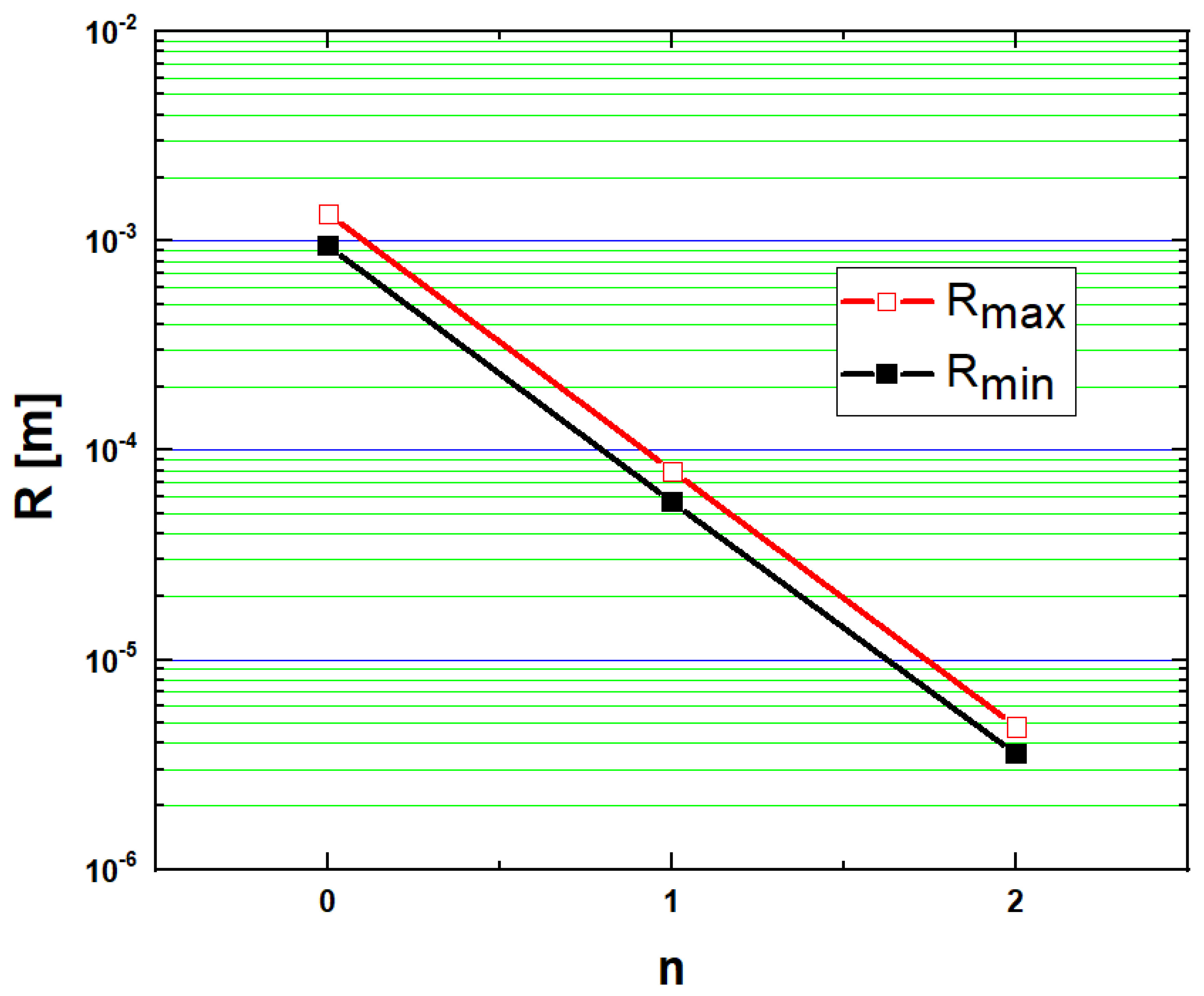
Figure 4.
Power law dependence of the velocity as a function of the distance to the corner.

Figure 5.
Red Vwall = 0.5 m/s and aspect ratio = 5; black Vwall = 0.005 m/s and aspect ratio = 1.

Figure 6.
Velocity magnitude close to the corner defined by a stationary and a moving wall; (red) Vwall = 0.5 m/s and aspect ratio = 5; (black) Vwall = 0.005 m/s and aspect ratio = 1.
Figure 6.
Velocity magnitude close to the corner defined by a stationary and a moving wall; (red) Vwall = 0.5 m/s and aspect ratio = 5; (black) Vwall = 0.005 m/s and aspect ratio = 1.
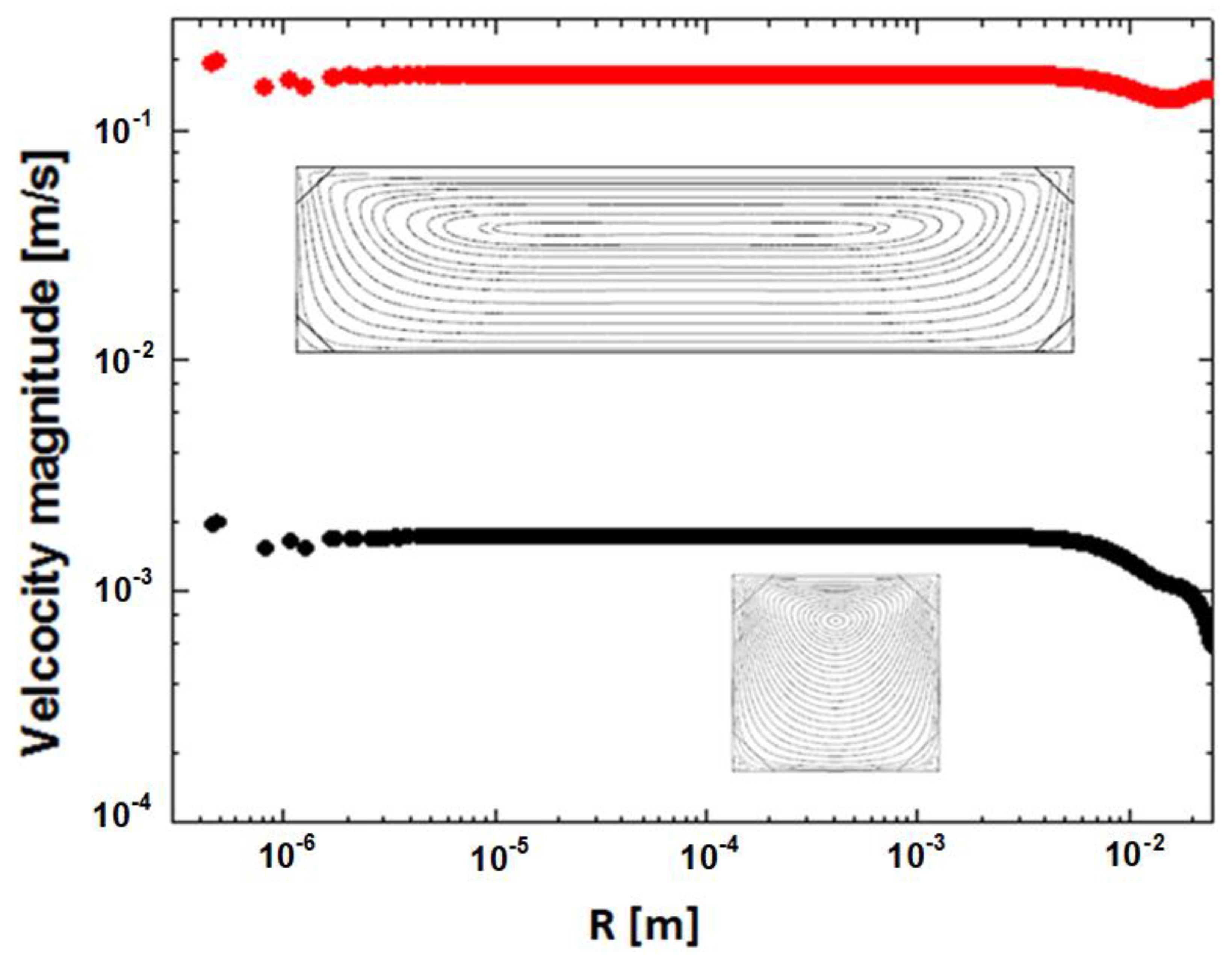
Figure 7.
Velocity cut across the central stagnation point (vwall = 0.005 m/s, aspect ratio = 1). The magnification close to the stagnation point shows the linear dependence of the velocity on the distance to the stagnation point.
Figure 7.
Velocity cut across the central stagnation point (vwall = 0.005 m/s, aspect ratio = 1). The magnification close to the stagnation point shows the linear dependence of the velocity on the distance to the stagnation point.

Publisher’s Note: MDPI stays neutral with regard to jurisdictional claims in published maps and institutional affiliations. |
© 2020 by the authors. Licensee MDPI, Basel, Switzerland. This article is an open access article distributed under the terms and conditions of the Creative Commons Attribution (CC BY) license (http://creativecommons.org/licenses/by/4.0/).
Share and Cite
MDPI and ACS Style
Kaufman, M.; Fodor, P.S. Analogy between Thermodynamic Phase Transitions and Creeping Flows in Rectangular Cavities. Symmetry 2020, 12, 1859. https://doi.org/10.3390/sym12111859
AMA Style
Kaufman M, Fodor PS. Analogy between Thermodynamic Phase Transitions and Creeping Flows in Rectangular Cavities. Symmetry. 2020; 12(11):1859. https://doi.org/10.3390/sym12111859
Chicago/Turabian StyleKaufman, Miron, and Petru S. Fodor. 2020. "Analogy between Thermodynamic Phase Transitions and Creeping Flows in Rectangular Cavities" Symmetry 12, no. 11: 1859. https://doi.org/10.3390/sym12111859
Note that from the first issue of 2016, this journal uses article numbers instead of page numbers. See further details here.