Abstract
Analog circuit fault diagnosis technology is widely used in the diagnosis of various electronic devices. The basic strategy is to extract circuit fault characteristics and then to use a clustering algorithm for diagnosis. The discrete Volterra series (DVS) is a common feature extraction method; however, it is difficult to calculate its parameters. To solve the problem of feature extraction in fault diagnosis, we propose an improved hierarchical Levenberg–Marquardt (LM)–DVS algorithm (IDVS). First, the DVS is simplified on the basis of the hierarchical symmetry of the memory parameters, the LM strategy is used to optimize the coefficients, and a Bayesian information criterion based on the symmetry of entropy is introduced for order selection. Finally, we propose a fault diagnosis method by combining the improved DVS algorithm and a condensed nearest neighbor algorithm (CNN) (i.e., the IDVS–CNN method). A simulation experiment was conducted to verify the feature extraction and fault diagnosis ability of the IDVS–CNN. The results show that the proposed method outperforms conventional methods in terms of the macro and micro F1 scores (0.903 and 0.894, respectively), which is conducive to the efficient application of fault diagnosis. In conclusion, the improved method in this study is helpful to simplify the calculation of the DVS parameters of circuit faults in analog electronic systems, and provides new insights for the prospective application of circuit fault diagnosis, system modeling, and pattern recognition.
1. Introduction
The diagnosis of circuit faults involves determining whether the circuit is working properly and identifying the location of fault components through the collected signals. It has been widely applied and studied in the fields of household appliances, medical electronic equipment, and automobile electronic equipment. An analog circuit is more difficult to diagnose than a digital circuit based on binary logic because of its continuous time signals, component tolerance, and nonlinearity. Therefore, it is necessary to develop an efficient diagnostic method to solve the production discontinuity due to machine circuit faults, in order to reduce the maintenance cost of electronic circuit systems [1,2,3,4].
In the process of analog circuit fault diagnosis, the collected circuit fault samples are typically processed in two steps: (1) Extracting the features, and (2) clustering the samples. The discrete Volterra series (DVS) model [4,5,6] is commonly used for feature extraction. However, with a linear increase in the order of the DVS, the number of parameters increases exponentially. Moreover, with the increase in the DVS order and cumulative layers, the structure complexity increases, making it even more difficult to calculate the DVS parameters. To date, scholars have proposed improved methods to simplify DVS parameter calculation, including the least-squares (LS) variant method, the frequency domain method, and the structure transformation method [7]. However, some problems remain. For example, the LS variant method is mainly aimed at improving the optimization strategy; it remains difficult to adjust the parameters in this common strategy, and this process is prone to local optimal problems [8,9,10]. Based on the frequency domain, the frequency domain method simplifies the parameter calculation, which is convenient for analysis and interpretation through charts. However, it has specific requirements for excitation and may lead to a dimensional disaster in the case of multidimensional properties [11,12,13,14]. In the structural transformation method, orthogonal basis functions are introduced to expand the DVS; although this method does not require specific input forms, it has strict constraints on poles, and the processing of these poles is complex [15,16,17]. Evidently, the improved parameter calculation methods for the DVS model have not been able to effectively solve the complexity problem in high-order parameter calculations.
Hierarchical design (HD) is an equivalent transformation scheme for DVS, based on the symmetric hierarchy of memory parameters. By merging items with the same memory parameters in each sub-item of the DVS, the DVS can be divided into items with the same number of memory lengths, all of which can be summed up to obtain the hierarchical DVS [18]. The advantage of the HD is that it transforms the complex DVS into multiple simple recursive terms. After the initial parameters of the recursive terms have been obtained, the recursion relationship can be used to obtain the recursion terms of the next layer, so as to avoid the separation of the parameter calculations of each order; this method has a higher data reuse rate than the conventional structure transformation method. In the parameter calculation of the hierarchical DVS, the optimization strategy also plays an important role in simplifying the parameter calculation. The Levenberg–Marquardt (LM) algorithm is an optimization strategy exhibiting fast convergence, less calculation, and adaptive parameter adjustment [19]. It combines the advantages of the gradient descent and Newton methods and is suitable for the parameter optimization of hierarchical DVS. After the optimal coefficient of the hierarchical DVS has been obtained through the LM strategy, the high-order DVS parameters can be calculated by substituting the coefficient into the parametric equation. However, the superiority of the model is not directly proportional to the order; for order selection, we should consider the balance between complexity and actual fitting precision. To this end, we introduced a Bayesian information criterion (BIC) [20] based on the symmetry of entropy to balance the model complexity and fitting effect. The BIC provides a basis for the order selection of hierarchical DVS.
This paper proposes an improved hierarchical DVS algorithm (IDVS). In our approach, the HD is used to simplify the DVS structure, the LM strategy is applied to efficiently search for the best coefficient, and the BIC is used to select the order, so as to solve the complex problem of DVS parameter calculation in the feature extraction step. Moreover, in step 2 (clustering) of circuit diagnosis, the most commonly used algorithms are support vector machines (SVMs), artificial neural networks (ANNs), decision trees (DTs), and condensed nearest neighbors algorithm (CNNs). Among them, the SVM model requires a difficult selection process for the appropriate kernel functions to solve nonlinear circuit problems [21] and does not directly support the classification of multi-class circuit faults. Neural networks take a long time to learn circuit fault samples, requiring many parameters [22]. When a DT is applied to time-ordered circuit fault response and highly correlated fault data, the effect of a decision depends on sample preprocessing [23]. Meanwhile, a CNN does not require estimating the parameters and has a short clustering time, making it more suitable for the clustering problem of multiple faults in nonlinear circuits [24].
To sum up, we propose an efficient analog circuit diagnosis method (IDVS–CNN) that combines the improved hierarchical DVS model with a CNN. The performance of the proposed method is tested by conducting a simulation experiment on uniform samples of a circuit. In the simulation experiment, three standard test circuits were taken as the object. The DVS and IDVS were used to extract the features of the circuit sample data, and the effects of the two methods were compared. The diagnostic effects of the CNN, DVS–CNN, and IDVS–CNN were also compared. The purpose of this study was to provide a new idea for the efficient diagnosis of circuit faults in analog electronic systems.
2. IDVS–CNN Algorithm Principle
2.1. IDVS Algorithm
2.1.1. Hierarchical DVS Model
The DVS is a functional series expansion of a nonlinear time-invariant system, which can be considered a generalization of 1D convolution in a multidimensional convolution space. The system output can be expressed as the sum of linear and nonlinear components:
where k is the time, m is the memory parameter, M + 1 is the memory length, hr is the kernel function of the r-order term, u is the input term, and the r-order term has r accumulation layers. Based on the hierarchical structure shown in Figure 1, the memory parameters are merged to realize the HD of the DVS. The IDVS model with only basic coefficients is obtained [18]:
where y0 = u(n).
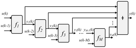
Figure 1.
Structure of the hierarchical design.
Equations (2) and (3) transform the double finite form (the memory parameter m and the order r are finite) of Equation (1) into a single finite form (the memory parameter M is finite), and the error due to the r-order truncation model is avoided.
The expressions of the IDVS first-order and r-order kernel parameters can be derived from the simultaneous Equations (1)–(3) [18]:
where:
β (0) and Λ (0) are equal to 1, and u(ρ-α) is a type of jump function:
2.1.2. Complexity of the Hierarchical DVS
In Equations (2) and (3), the hierarchical DVS consists of M stages, each having only three multiplication and three addition operations, amounting to only 6M operations, and the complexity of the model is O (M).
For the DVS model, if the calculation is mainly consumed by multiplication, its expansion requires TDVS multiplication [18]:
In other words, the complexity of the DVS model is O (2M).
From the viewpoint of parameter hr, the IDVS directly provides the parameter calculation, i.e., Equation (4), of each order and the relationship, i.e., Equation (5), between the parameters of each order. To calculate the parameters of each order, we only need to carry out the continuous multiplication and single-layer accumulation operation on the foundation coefficients [ai, bi, ci, di] of each layer. However, the DVS does not have an explicit parameter calculation equation, so the input matrix needs to be constructed during calculation. The matrix needs to be reconstructed every time an order is added, and the dimension of the matrix increases as the order of the model increases, which is not conducive to the implementation of the calculation program.
Therefore, from the aspects of model implementation and parameter calculation, the IDVS model requires fewer computation steps than the DVS.
2.1.3. LM Optimization of the Hierarchical DVS
From Equations (4)–(9), we find that the IDVS parameter equation is only related to the foundation coefficient. To estimate the parameter, we need to estimate the coefficients first: θ = [a b c d]T, where a = [a1 a2…aM]T, b = [b1 b2…bM]T, c = [c1 c2…cM]T, and d = [d1 d2…dM]T.
To obtain the optimal coefficient θopt, we introduced the LM optimization strategy. The LM algorithm searches for the best coefficient through the following iteration:
where λ is the adjustment factor, I is the unit matrix, R is the residual, and J is the Jacobian matrix.
To calculate the Jacobian matrix, we needed to calculate the partial derivative of the hierarchical DVS relative to θ, m = 1, 2, …, M. By induction, we derived the partial derivative equation of the hierarchical DVS as follows:
where si = ai+ciu(k-i), i ≥ 2, and μ1 = [u(k) y1(k) y2(k)…yM-1(k)].
Similarly:
where μ2 = [u(k-1) u(k-2)…u(k-M)], y (k) represents the total response of the IDVS, and yi (k) represents the response of the IDVS in the i-th stage.
The gradient of the IDVS is as follows:
where k = 1, 2, …, N.
Thus, the Jacobian matrix is:
The steps to search for the best coefficient are as follows:
- (i)
- Initialize the adjustment factor λ, coefficient θ1(0), input matrices μ1 and μ2, and Jacobian matrix J.
- (ii)
- Calculate the trial iteration step size step_try using Equation (19).
- (iii)
- Calculate the trial coefficient θ_try = θ-step_try.
- (iv)
- Put θ_try substituting Equations (2) and (3) to obtain y_hat, and calculate the chi-square error χ2_try.
- (v)
- Calculate the judgment factor ρ using Equation (21).
- (vi)
- If ρ is greater than 0.01, update the adjustment factor using Equation (22) and accept θ_try, χ2_try and update the iteration matrix J; otherwise, update the adjustment factor using Equation (23).
- (vii)
- Repeat steps ii–vi until the mean squared error (MSE) meets the set value or the iteration number reaches the upper limit; finally, the optimal parameters θopt are obtained.
2.1.4. Feature Extraction
The principle of DVS as a feature extraction method involves applying an excitation signal u (n) to the circuit, obtaining a response signal Y (n) in its output, making Y (n) equal to the output y (n) of the DVS, and substituting the excitation u (n) and response y (n) into the parameter equation of the DVS. Thus, the approximate transfer function of the circuit is obtained. The transfer function depends on the circuit structure. This is the basis of the hierarchical DVS as a feature extraction method.
The optimal foundation coefficient θopt was obtained using the method described in Section 2.1.3. We then substituted this into Equations (4) and (5) to obtain the first-order kernel h1 and the rest kernel hi (i = 2, …, r). [h1, h2, …, hr] was considered the eigenvector of the circuit.
When the order of the hierarchical DVS algorithm is 4, M = 20, the number of kernel parameters is 7545. Evidently, only a few of these parameters have a significant contribution to the system output. Therefore, principal component analysis (PCA) was applied to ignore items that have less contribution to the system output, so as to obtain the principal components of the eigenvector.
2.1.5. Order Selection of the Hierarchical DVS
As the order of the model increases, its fitting ability becomes stronger; however, it also becomes more complex. Therefore, it is necessary to appropriately choose the order of the IDVS to balance the fitting ability and complexity. Thus, the BIC criterion was introduced for order selection:
where k is number of model parameters, N is the number of samples, and σ2_hat is the likelihood function, k = (M+1)!/((r-1)!(M+1-r)!). The lower the BIC value, the better the model of the corresponding order. When the order r increases, k increases, and the likelihood function increases. There is a range of r values to minimize the BIC.
2.2. CNN Algorithm
Compression: The training set was divided into set A and set B, and the initial set A was empty.
We randomly took a sample from training set and placed it in A. If it could correctly classify the j-th sample in B (as follows), the j-th sample was kept in B; otherwise, it was placed in A. The above steps were repeated until all of the samples that could be correctly classified were retained in B.
Classification: The sampling data were divided into training and test sets. Let x be an n-dimensional vector sample of the test set, and y be an n-dimensional vector of the training set. We calculated the distance from x to all of the samples of the training set and sorted these distances from small to large. The samples of the first k distances are called k neighbors of x. The category frequency of k neighbors are calculated, and the category with the highest frequency is considered the category of x.
3. IDVS–CNN Diagnostic Procedures
The steps involved in analog circuit fault diagnosis based on the IDVS–CNN are as follows, and the block diagram of the proposed method is shown in Figure 2:
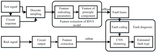
Figure 2.
Fault diagnosis implementation: Block diagram of the improved discrete Volterra series (IDVS)–condensed nearest neighbor algorithm (CNN).
- (i)
- Excitation u (n) is applied to the circuit and u (n) is saved, and the sample set of the circuit response in the normal state and the fault state [normal, fault_1, … fault_N] are collected.
- (ii)
- The IDVS algorithm is used to calculate the characteristic parameter set [h(NF), h(F1), …, h(Fi), …, h(FN)] of the circuit in each state; h (Fi) is the eigenvector of the circuit state I. r and M are set appropriately and the dimension of the parameters through PCA is reduced.
- (iii)
- The feature parameter set is used as the input to the CNN to build a diagnosis model, where the fault code is set as [normal, fault_1, …, fault_N] = [0, 1, 2 …, N], and k is set to the appropriate value.
- (iv)
- After calculating the IDVS characteristic parameter h(Fx) of the circuit response data under test, PCA is applied to reduce the dimension.
- (v)
- The characteristic parameters are input to the CNN model established in step (iii), and the corresponding fault mode code of the circuit under test is obtained.
4. Simulation Verification of the Improved Algorithm
4.1. Simulated Hardware Equipment
- CPU: Core i5-2450m 2.5 GHz.
- RAM memory: 4 G DDR3 1600.
- Hard disk: 1 TB.
- Software platform: MATLAB 2014B, PSpice 16.6.
4.2. Fault Mode
To test the performance of the IDVS–CNN circuit fault diagnosis algorithm, the biquad low-pass filter (BLPF) circuit, shown in Figure 3, was also taken as the object of the diagnosis experiment. For BLPF, 2 * 12 + 1 = 25 faults (including no fault states) can be defined for a single fault (the value of a single component increases or decreases). When the excitation is a unit amplitude alternate current (AC) signal, the output voltage (effective value) without a fault is 0.5405 V, and the output voltage of other faults is in the range of 0.4129–0.6469 V. According to the definition of a fuzzy group by Hochward et al. [25] (when the absolute value of the voltage difference between two faults is less than 0.7 V, the two faults belong to the same fuzzy group and cannot be distinguished), we can establish that all fault states belong to a fuzzy group. At this time, we can increase the measuring point or make full use of the information of a measuring point and process it; thus, fault diagnosis can be carried out. The method in this study considers the latter technique, which uses IDVS and CNN to process the fault information of a test point (output port). Through sensitivity analysis, the components with the lowest sensitivity were selected for the fault diagnosis test, and the others were tested in a similar manner. The lowest sensitivity implies that it is the least separable from the fault free state. If our method is effective for faults of a low sensitivity element, then it is also effective for faults of a high sensitivity component [26]. Therefore, we selected the resistors R1 and R2 and capacitors C1 and C2, which have a significant impact on the circuit response, for the diagnostic experiment. The fault modes were NF (no fault), R1↑, R1↓, R2↑, R2↓, C1↑, C1↓, C2↑, and C2↓, and the fault codes were NF, F1, F2, F3, F4, F5, F6, F7, and F8. ↑ means that the component has a 20% higher numerical fault, ↓ means that the component has a 20% lower numerical fault. The component tolerance was 10%.
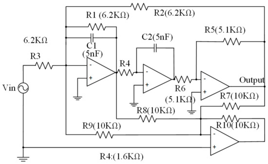
Figure 3.
Biquad low-pass filter (BLPF) circuit.
4.3. Diagnostic Test Process
The PSpice script was used to set the fault mode one element at a time, and the rest of the elements were nominal values with a tolerance of 10%. The Monte Carlo method was used to scan the BLPF in the above nine modes. An AC signal of the unit amplitude was set as the excitation. The scanning iteration was 50, the sampling time was 5 ms, the sampling step size was 25 µs, and the excitation signal was saved. Thus, a total of 450 data samples of nine modes were obtained (see Data S1 in Supplementary Materials), as shown in Figure 4a. Each sample had voltage response data of a length of 200.
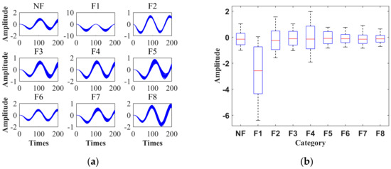
Figure 4.
BLPF sample data: (a) Original signal; (b) sample distribution.
The collected samples were input into MATLAB. The diagnostic procedure is shown in Section 3. First, the IDVS parameters were calculated. Second, dimensionality reduction was carried out using PCA. A three-fold test method was adopted to conduct diagnostic experiments. In other words, the feature samples of each mode were divided into three parts. We took two thirds of the samples as the training set (300 samples) and the remaining one third (150 samples) as the test diagnosis set. Figure 4b shows the sample distribution. The difference between the samples was the basis for identifying the fault category.
4.4. IDVS Order Selection
Taking the BLPF as the object, we used the IDVS of order 1 to calculate the parameters, and the response was reconstructed with the obtained parameters. Here, we took 1/MSE as the likelihood function and used Equation (24) to calculate the BIC. Figure 5 shows the statistical test results. As shown in Figure 5, the BIC gradually decreased as the order increased and tended to be stable when r = 4. This indicates that when the order of the IDVS model is set as 4, the complexity and BLPF fitting accuracy are balanced optimally.
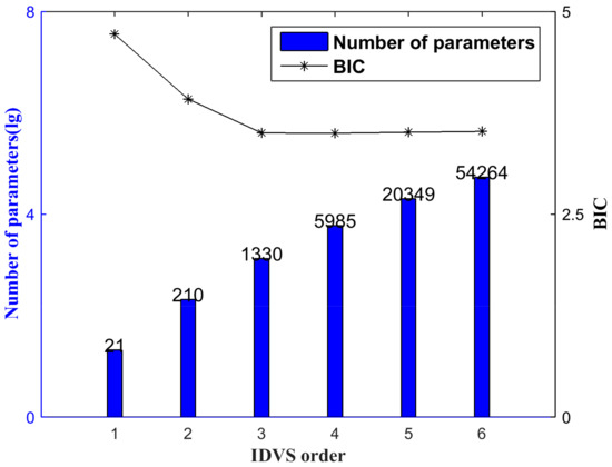
Figure 5.
IDVS order selection of BLPF. BIC, Bayesian information criterion.
4.5. LM Optimization of Coefficients
In the process of determining the optimal IDVS coefficient of each fault sample using the LM algorithm (see Code S1 in Supplementary Materials), the estimated signal corresponding to the optimal coefficient is shown in Figure 6b (Data S2). Figure 6a shows the estimated signal of the LS algorithm (Data S3). The MSE comparison in Figure 6c shows that the LM algorithm has high optimization accuracy (Data S4 and S5).
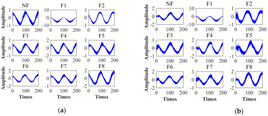
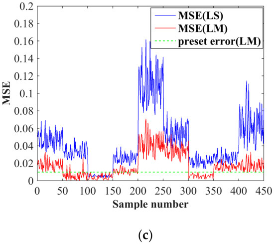
Figure 6.
Coefficient optimization comparison. (a) Output estimation of the least-squares (LS) algorithm; (b) output estimation of the Levenberg–Marquardt (LM) algorithm; (c) mean square error (MSE) comparison of the LS and LM algorithms.
4.6. Calculation of the Characteristic Parameters
After the optimal coefficient of the fault modes NF–F8 were obtained, the characteristic parameters h1–h4 (Data S6–S9) of orders 1–4 were obtained using the parameter calculations in Equations (4)–(9) of the IDVS (Codes S2–S5), as shown in Figure 7a–d. By expanding the parameters of each order into a vector and combining them into a vector, we obtained the eigenvector [h1 h2 h3 h4] (Data S10), as shown in Figure 8.
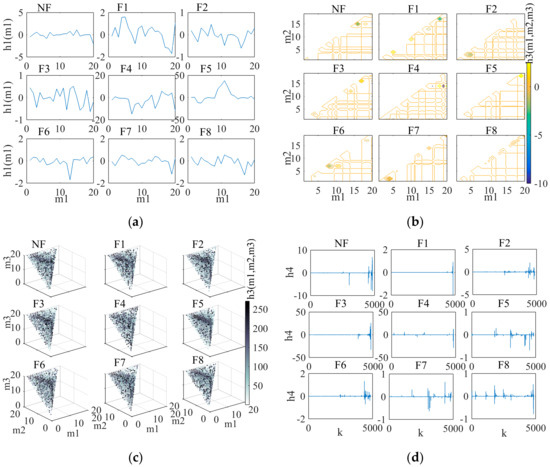
Figure 7.
Comparison of the characteristic parameters of each state. (a) h1; (b) h2; (c) h3; (d) h4. Note: h4 is the result of five-dimensional data h4 (m1, m2, m3, m4) expanded into a vector.
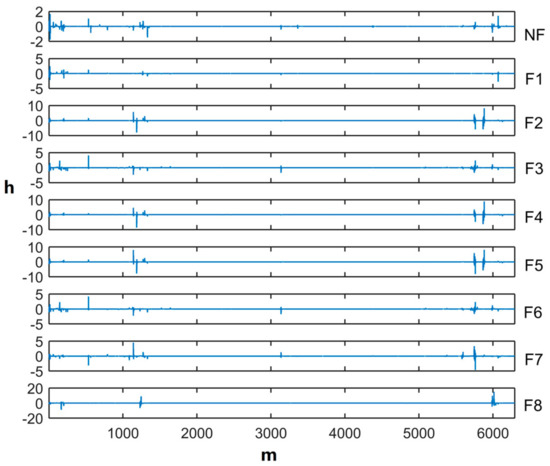
Figure 8.
Comparison of eigenvector h of each state.
After the IDVS was used to calculate the eigenvector of the sample, PCA was applied to analyze the eigenvector and to obtain 3D feature samples. The original data, eigenvector [h1 h2], and eigenvector [h1 h2 h3 h4] were compared (Data S11–S13), as shown in Figure 9a–c. In Figure 9a, the primary components of each fault mode overlap considerably. In Figure 9b, the fault modes R1↑, R2↑, R1↓, and R2↑ have distinct principal components, and the capacitive faults C1↑, C2↑, C1↓, and C2↓ still have a high overlap. In Figure 9c, the capacitive faults are further separated.
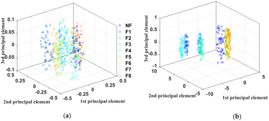
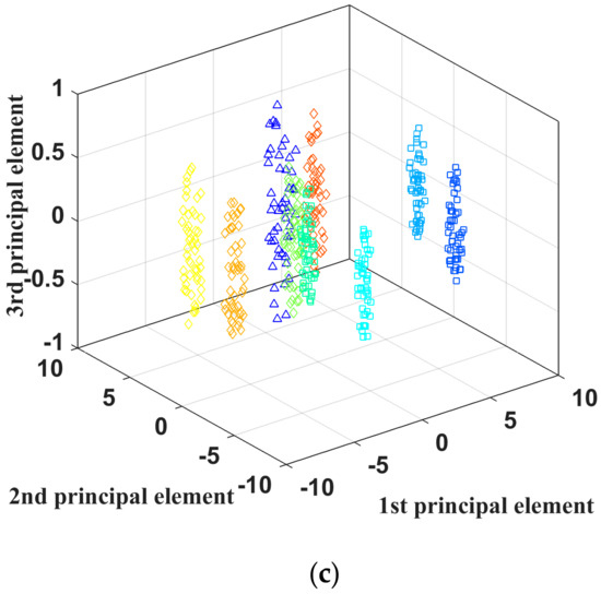
Figure 9.
Principal component comparison of the eigenvectors. (a) Principal component of the raw data; (b) principal components of the DVS eigenvectors (r = 2); (c) principal component of the IDVS eigenvectors (r = 4).
The main reason was the high similarity between the circuit responses in each fault mode (as shown in Figure 4). After extracting the features by DVS (r = 2), we obtained the approximate parameters reflecting the characteristics of the circuit. However, because of the computational complexity, the model usually only takes an order 2, thus limiting the fitting accuracy of the DVS. With the IDVS for feature extraction, we were able to set the model order as 4, thereby improving the model fitting accuracy and feature extraction effect.
4.7. Distance Calculation
After the eigenvector was obtained, the inter- and between-class distances corresponding to the eigenvector [h1 h2 h3 h4] were calculated using (22) of the CNN algorithm. Figure 10 shows a comparison of the eigenvector [h1 h2 h3 h4] with the original data y_dat and commonly used eigenvector [h1 h2].
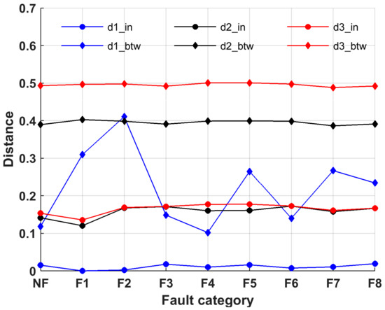
Figure 10.
Comparison of the inter- and between-class distances. Note: d1, d2, and d3 are the distances of the original signal, feature [h1 h2], and feature [h1 h2 h3 h4] of fault modes NF–F8, respectively.
Figure 10 shows that when [h1 h2 h3 h4] was used as the eigenvector, the average between-class distance _btw of the corresponding mode was 0.5, while the average inter-class distance _in was approximately 0.16, _btw > _btw(0.39) > _btw(0.22) (Data S14–S16), and _in ≈ _in > _in(0.01) (Data S17–S19). The difference Δ d between the between-class distance and the inter-class distance determines the classification performance of the eigenvector. Because Δ d (3) > Δ d (2) > Δ d (1), the eigenvector [h1 h2 h3 h4] has a better classification performance.
4.8. Comparison of the Diagnostic Effects
For the above circuits and their fault modes, the CNN, DVS–CNN, and IDVS–CNN were used for diagnosis comparison. Figure 11 shows the diagnostic results in the form of a confusion matrix (Data S20–S22).
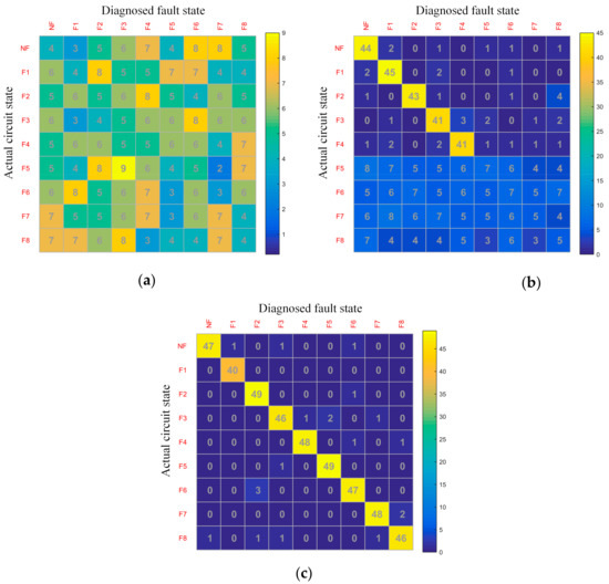
Figure 11.
Diagnosis results of the BLPF circuit: (a) CNN algorithm; (b) DVS–CNN algorithm; (c) IDVS–CNN algorithm.
Figure 11 shows that the confusion matrix corresponding to the CNN algorithm is diagonally fuzzy and that the fault mode misdiagnosis is considerable (Figure 11a). In the confusion matrix of the DVS–CNN algorithm, the diagnosis effect of F1–F4 modes is evident, whereas the misdiagnosis of the F5–F8 modes is still considerable (Figure 11b). The confusion matrix of the IDVS–CNN has clear diagonals, indicating that it has a low misdiagnosis rate and a good fault diagnosis effect (Figure 11c).
To evaluate the diagnosis effect of the various circuit diagnosis algorithms more objectively and reasonably, the indexes used to evaluate the diagnosis effect were calculated from the confusion matrix shown in Figure 11, including the prediction accuracy with fault (S1), prediction accuracy without fault (S2), error rate (S3), macro F1 score (macroF1), and micro F1 score (microF1) [27]. The single fault diagnosis time was counted.
Table 1 shows that the IDVS–CNN method outperforms the other methods in terms of the first five indicators. The main reason is that when the CNN deals with samples with evident aliasing features, the clustering effect is affected by the characteristic aliasing samples.

Table 1.
Diagnostic performance of IDVS compared to the other algorithms.
The DVS–CNN algorithm is limited by the high complexity of the DVS parameters and only uses the first two order parameters. The IDVS–CNN uses hierarchical DVS for parameter calculation, with a much lower complexity when calculating the order 4 model parameters. Moreover, it can effectively expand the feature differences between the fault modes and can strengthen the aggregation of the features of the same category (as shown in Figure 9c), thus improving the diagnostic capability of the CNN algorithm.
Furthermore, the average diagnosis time of the IDVS–CNN is lower than that of the DVS–CNN, while the diagnosis effect is better. The reason is that the IDVS uses high-order parameters, which have a low computational complexity.
In order to verify the effectiveness of this method, a more complex integrated operational amplifier circuit was used, as shown in the Figure 12. The circuit consisted of 20 transistors, 11 resistors, and a capacitor. Similar to the previous experiment, according to the fuzzy group and testability analysis, we divided all single fault states into the same fuzzy group when only the output end was selected as the measuring point. The components with the lowest sensitivity were selected as the key components for the fault diagnosis test experiment, and the rest of the components were tested in the same way. Thus, five components (i.e., Q1, Q9, Q11, Q18, and R1) were selected for the fault test, and there were 10 fault modes (the value of a single component increases or decreases). The analysis method for the other fault conditions was the same as that for these 10 types of faults. The transistor failure mode is defined by the percentage of change in the ideal maximum reverse beta β; this parameter is affected by the internal structure and temperature of the transistor. When β increases by 20% relative to the nominal value, it is recorded as Q¾↑, and as Q↓ when it decreases by 20%. The failure modes included Q1↑, Q1↓, Q9↑, Q9↓, Q11↑, Q11↓, Q18↑, Q18↓, R1↑, and R1↓ (Data S23). The excitation voltage was added to the non-inverting port, and the response voltage was collected at the output port; the diagnostic test was the same as that in the previous experiment. The statistical results of the diagnosis are shown in Table 2.
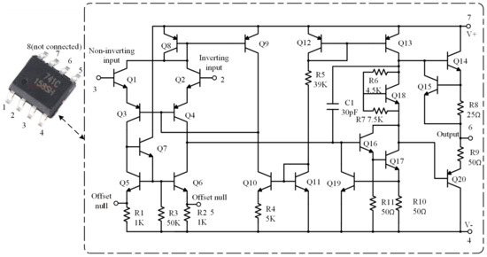
Figure 12.
Integrated operational amplifier (µA741). Note: The left is a physical picture of the circuit, and the right is an equivalent circuit diagram.
Table 2.
Diagnosis results of the different methods.
It can be seen from Table 2 that when the signal-to-noise ratio (SNR) decreases, that is, the proportion of noise in the collected signal increases, the diagnostic rate of the four methods clearly decreases. However, the diagnostic rate of the proposed method is better than that of the other three methods under three noise levels. When the SNR is as low as 10 dB, this method still has a 76% diagnosis rate. At the same time, the diagnosis time consumption of this method is comparable to that of the other methods. The reason behind this is that this method is based on the DVS model and uses the input and output signals to solve the circuit characteristics, which has stronger noise robustness. In addition, the hierarchical method combined with the LM strategy was used to simplify the calculation of DVS parameters, which reduced the calculation time of the high-order DVS parameters.
4.9. Real Circuits Experiment
The equipment shown in Figure 13 was used to test the benchmark circuit continuous-time state variable filter (CTSVF) (as shown in Figure 14), in which the CTSVF fault was set by jumping cap. Similar to the previous experiment, through sensitivity analysis combined with fuzzy group and testability, the components with the lowest sensitivity (R1, R3, and C2) were selected as the key components for the fault diagnosis test experiment, and the rest of the components were tested in the same way. The experimental results are shown in Table 3. The accuracy indexes of the CTSVF diagnosis results for S1, S2, macroF1, microF1, and time cost are 91%, 92%, 2.4%, 0.875, 0.891, and 11.2 s, respectively. The results show that the proposed method is useful for discriminating fault components and fault categories, regardless of their variations in tolerance in the analog circuit.
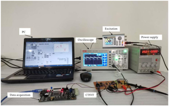
Figure 13.
Experimental equipment.
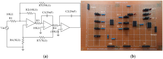
Figure 14.
Continuous-time state variable filter (CTSVF) circuit. (a) Schematic diagram; (b) test board.
Table 3.
Diagnosis results of CTSVF.
Analog filter circuits (i.e., CTSVF and BLPF shown in Figure 3 and Figure 14) are widely used in electronic devices as indispensable components in the signal preprocessing stage. Recently, there have been a lot of related literature works on analog circuit fault diagnosis based on these two circuits [22,26,28,29,30]. Our experimental results show that the proposed method is effective for the diagnosis of these two circuits and has the advantage of noise robustness compared to several mainstream methods. In addition, a multistage AC amplifier (Figure 15) used in various electronic devices was added and then a diagnostic statistical experiment was carried out on this circuit. The results show that the average diagnostic rates for randomly selected fault modes (i.e., RB1↑, RB1↓, RB21↑, RB21↓, RF↑, RF↓, RL↑, RL↓) are 87%, 85%, 82%, 88%, 89%, 88%, 89%, and 85%, respectively. This further demonstrates the effectiveness of our method in engineering applications.
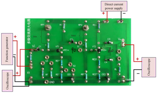
Figure 15.
Multistage alternate current (AC) amplifier.
5. Conclusions
To overcome the difficulty in calculating the DVS parameters for analog circuit fault diagnosis, we developed an efficient fault diagnosis algorithm based on the IDVS–CNN. Based on the hierarchical IDVS, the LM was used to find the optimal coefficient, and an IDVS parametric equation containing only the foundation coefficient was then used to extract the fault characteristics from the analog circuit data. The analog circuit fault diagnosis was realized by combining IDVS with the CNN algorithm. The experimental results show that the algorithm retains the excellent feature extraction ability of the DVS, reduces the steps required for calculating the DVS parameters, and shows better diagnostic performance. This study simplifies the calculation of the DVS parameters of circuit faults in analog electronic systems and provides new ideas for efficient circuit diagnosis.
It is worth mentioning that we derived the relative partial derivative equation of the hierarchical DVS model, which enabled us to use an optimization strategy (LM algorithm) to solve the parameters of the hierarchical DVS. The experiment proved that this strategy has a lower error in parameter solving than the traditional LS strategy. Furthermore, the BIC criterion was introduced to provide the basis for order selection of the DVS, and the experiments show that there is an order range to balance the complexity and accuracy of the model. Finally, by combining the LM strategy, hierarchical DVS, BIC criteria, and the CNN clustering algorithm, we proposed the IDVS–CNN analog circuit fault diagnosis method. The experiments showed that this method has a better diagnosis effect than the previous DVS–CNN method on small circuits and has an advantage over several mainstream methods in dealing with more complex integrated circuits and high noise interference. In the future, we intend to implement the algorithm on portable devices, so as to break away from PC dependence and enhance the applicability of this method.
Supplementary Materials
The following are available online at https://www.mdpi.com/2073-8994/12/11/1901/s1. The original data of Figure 4 is shown in Data S1, and the original data of Figure 6, Figure 7, Figure 8, Figure 9, Figure 10 and Figure 11 are shown in Data S2–S22. The source code of the IDVS parameter calculation part is shown in Codes S1–S5.
Author Contributions
Y.D. conceptualized the main idea of this project; Y.Z. proposed the method and designed the work, then conducted the experiments and analyzed the data; Y.Z. wrote the whole paper; Y.D. reviewed and edited the paper. All authors have read and agreed to the published version of the manuscript.
Funding
This work was supported by the Sichuan Science and Technology Support Program (2017FZ0033), Key Scientific Research Projects of Sichuan Education Department (13ZA0186).
Conflicts of Interest
The authors declare no conflict of interest.
References
- Bandler, J.; Salama, A. Fault diagnosis of analog circuits. Proc. IEEE 1985, 73, 1279–1325. [Google Scholar] [CrossRef]
- Li, F.; Woo, P. Fault detection for linear analog IC—The method of short-circuits admittance parameters. IEEE Trans. Circuits Syst. I Regul. Pap. 2002, 49, 105–108. [Google Scholar]
- Yang, S.; Hu, M.; Wang, H. Study on Soft Fault Diagnosis of Analog Circuits. Microelectron. Comput. 2008, 25, 1–8. [Google Scholar]
- Binu, D.; Kariyappa, B. A survey on fault diagnosis of analog circuits: Taxonomy and state of the art. Int. J. Electron. Commun. 2017, 73, 68–83. [Google Scholar] [CrossRef]
- Tang, H.; Liao, Y.; Cao, J.; Xie, H. Fault diagnosis approach based on Volterra models. Mech. Syst. Signal Process. 2010, 24, 1099–1113. [Google Scholar] [CrossRef]
- Cheng, C.; Peng, Z.; Zhang, W.; Meng, G. Volterra-series-based nonlinear system modeling and its engineering applications: A state-of-the-art review. Mech. Syst. Signal Process. 2017, 87, 340–364. [Google Scholar] [CrossRef]
- Peng, Z.; Cheng, C. Volterra series theory: A state-of-the-art review. Chin. Sci. Bull. 2015, 60, 1874–1888. [Google Scholar]
- Jiang, B.; Yang, J.; Zhang, E. QRD-RLS Algorithm for Sparse Adaptive Volterra filtering. Signal Process. 2008, 24, 595–599. [Google Scholar]
- Laura, D.; Jurair, D.; Luis, T. Efficient Volterra systems identification using hierarchical genetic algorithms. Appl. Soft. Comput. J. 2019, 85, 105745. [Google Scholar]
- Chang, W. Volterra filter modeling of nonlinear discrete time system using improved particle swarm optimization Digital. Signal Process. 2012, 22, 1056–1062. [Google Scholar]
- Li, M.; Billings, S. Piecewise Volterra modeling of the Duffing oscillator in the frequency-domain. Mech. Syst. Signal Process. 2012, 26, 118–127. [Google Scholar] [CrossRef]
- Cao, J.; Chen, L.; Zhang, J. Fault diagnosis of complex system based on nonlinear frequency spectrum fusion. Measurement 2013, 46, 125–131. [Google Scholar] [CrossRef]
- Cheng, C.; Peng, Z.; Dong, X.; Zhang, W.; Meng, G. Locating non-linear components in two dimensional periodic structures based on NOFRFs. Int. J. Non-Linear Mech. 2014, 67, 198–208. [Google Scholar] [CrossRef]
- Liu, Y.; Li, J. A novel fault diagnosis method for rotor rub-impact based on nonlinear output frequency response functions and stochastic resonance. J. Sound Vib. 2020, 481, 11541. [Google Scholar] [CrossRef]
- Garna, T.; Bouzrara, K.; Ragot, J.; Messaoud, H. Nonlinear system modeling based on bilinear Laguerre orthonormal bases. ISA Trans. 2013, 52, 301–317. [Google Scholar] [CrossRef]
- Luis, G.; Samuel, D.; Americo, C. Damage detection in uncertain nonlinear systems based on stochastic Volterra series. Mech. Syst. Signal Process. 2019, 125, 288–310. [Google Scholar]
- Koen, T.; Johan, S. Wiener system identification with generalized orthonormal basis functions. Automatica 2014, 50, 3147–3154. [Google Scholar]
- Mohsen, A.; Nadia, N. Practical realization of discrete-time Volterra series for high-order nonlinearities. Nonlinear Dyn. 2019, 98, 2309–2325. [Google Scholar]
- Ameer, A.; Atherton, W.; Rafid, M.; Khalid, R. Performance analysis of an evolutionary LM algorithm to model the load-settlement response of steel piles embedded in sandy soil. Measurement 2019, 140, 622–635. [Google Scholar]
- Zhao, J.; Jin, L.; Shi, L. Mixture model selection via hierarchical BIC. Comput. Stat. Data Anal. 2015, 88, 139–153. [Google Scholar] [CrossRef]
- Cao, J.; Wang, D.; Qu, Z.; Sun, H.; Li, B.; Chen, C.-L. An Improved Network Traffic Classification Model Based on a Support Vector Machine. Symmetry 2020, 12, 301. [Google Scholar] [CrossRef]
- Zhao, G.; Liu, X.; Zhang, B.; Liu, Y.; Niu, G.; Hu, C. A novel approach for analog circuit fault diagnosis based on Deep Belief Network. Measurement 2018, 121, 170–178. [Google Scholar] [CrossRef]
- Liu, W.; Deng, K.; Zhang, X.; Cheng, Y.; Zheng, Z.; Jiang, F.; Peng, J. A Semi-Supervised Tri-CatBoost Method for Driving Style Recognition. Symmetry 2020, 12, 336. [Google Scholar] [CrossRef]
- Liang, T.; Xu, X.; Xiao, M. A new image classification method based on modified condensed nearest neighbor and convolutional neural networks. Pattern Recognit. Lett. 2017, 94, 105–111. [Google Scholar] [CrossRef]
- Sara, S.; Seyyed, H.; Mahdi, E. Optimum test point selection method for analog fault dictionary techniques. Analog. Integr. Circuits Signal Process. 2019, 100, 167–179. [Google Scholar]
- Liu, Z.; Liu, T.; Han, J.; Bu, S.; Tang, X.; Michael, P. Signal Model-Based Fault Coding for Diagnostics and Prognostics of Analog Electronic Circuits. IEEE Trans. Ind. Electron. 2017, 64, 605–614. [Google Scholar] [CrossRef]
- Liu, L.; Wang, W. An efficient instance selection algorithm to reconstruct training set for support vector machine. Knowl. Based Syst. 2017, 166, 58–73. [Google Scholar] [CrossRef]
- Yuan, Z.; He, Y.; Yuan, L.; Cheng, Z. A Diagnostics Method for Analog Circuits Based on Improved Kernel Entropy Component Analysis. J. Electron Test. 2017, 33, 697–707. [Google Scholar] [CrossRef]
- He, W.; He, Y.; Li, B. Generative Adversarial Networks with Comprehensive Wavelet Feature for Fault Diagnosis of Analog Circuits. IEEE Trans. Instrum. Meas. 2020, 69, 6640–76650. [Google Scholar] [CrossRef]
- Zhao, D.; He, Y. A novel binary bat algorithm with chaos and Doppler effect in echoes for analog fault diagnosis. Analog. Integr. Circuits Signal Process. 2016, 87, 437–450. [Google Scholar] [CrossRef]


Publisher’s Note: MDPI stays neutral with regard to jurisdictional claims in published maps and institutional affiliations. |
© 2020 by the authors. Licensee MDPI, Basel, Switzerland. This article is an open access article distributed under the terms and conditions of the Creative Commons Attribution (CC BY) license (http://creativecommons.org/licenses/by/4.0/).