Unsupervised Clustering for Hyperspectral Images


The Machine Intelligence and Information Visualization Lab (MintViz), Integrated Center for Research, Development and Innovation in Advanced Materials, Nanotechnologies, and Distributed Systems for Fabrication and Control (MANSiD) Research Center, Faculty of Electrical Engineering and Computer Science, Stefan cel Mare University, No. 13, Str. Universitatii, 720229 Suceava, Romania
*
Authors to whom correspondence should be addressed.
†
Current address: “Stefan cel Mare” University, Faculty of Electrical Engineering and Computer Science, No. 13, Str. Universitatii, 720229 Suceava, Romania.
Symmetry 2020, 12(2), 277; https://doi.org/10.3390/sym12020277
Submission received: 17 January 2020
/
Revised: 4 February 2020
/
Accepted: 7 February 2020
/
Published: 12 February 2020
Abstract
:Hyperspectral images are becoming a valuable tool much used in agriculture, mineralogy, and so on. The challenge is to successfully classify the materials founded in the field relevant for different applications. Due to a large amount of data corresponding to a big number of spectral bands, the classification programs require a long time to analyze and classify the data. The purpose is to find a better method for reducing the classification time. We exploit various algorithms on real hyperspectral data sets to find out which algorithm is more effective. This paper presents a comparison of unsupervised hyperspectral image classification such as K-means, Hierarchical clustering, and Parafac decomposition, which allows the performance of the model reduction and feature extraction. The results showed that the method useful for big data is the classification of data after Parafac Decomposition.
1. Introduction
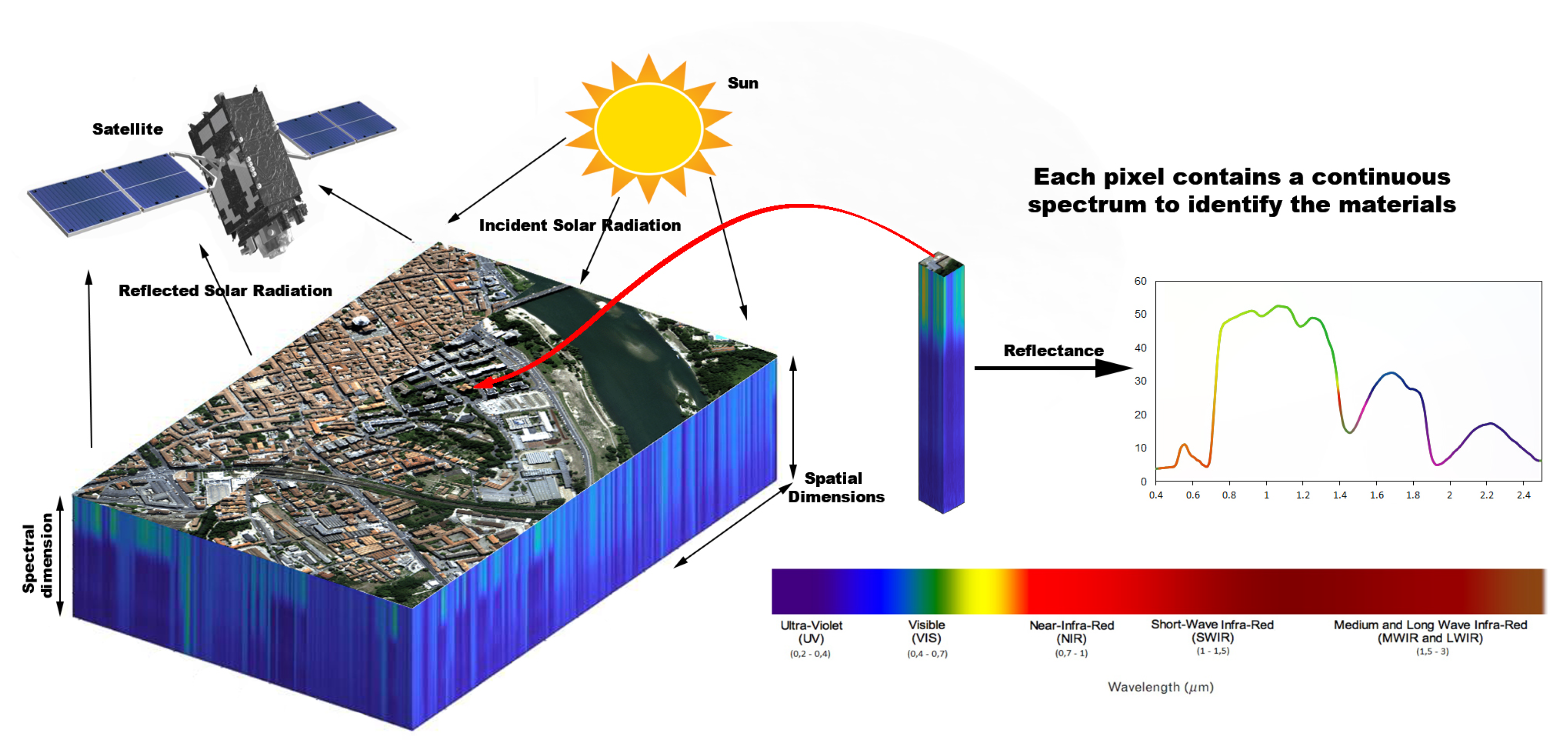
Hyperspectral images are a challenging area due to unfavorable resolution of images, high dimensionality, and insufficient ground truth data during training. Hyperspectral systems acquire images in about a hundred or more continuous spectral bands [see Figure 1]. At different wavelengths, the materials reflect and absorb differently. If the detection system has sufficient spectral and spatial resolution, the materials can be identified from their spectral signatures [1]. The unsupervised classification discovers the information on its own and also leaves the number of classes to be chosen by the user.
Hyperspectral image classification is very complex and difficult to obtain because of image noises, complex background, various characters [2] or high dimensionality [3]. Each pixel is assigned to a class, leaving the user to find the meaning for each class. Also, existing classifiers do not always offer a better classification for all types of data, which is why studying the classification of hyperspectral images can provide us general information about classification accuracy. Hyperspectral images are an important tool for identifying materials spectrally unique, as it provides sufficient information for classifying data from different areas. Furthermore, hyperspectral images could be used to caption the different phases of the eruptive activity of volcanoes, to obtain a detailed chronology of the lava flow emplacement and radiative power estimation [4].
In Reference [6], unsupervised algorithms (means K and ISODATA) were applied to hyperspectral images and, although both gave accurate results, K-means had better results. Another approach of hyperspectral classification is described in Reference [7], where the authors used Maximum Likelihood (ML), Spectral Angle Mapper (SAM), and Support Vector Machine (SVM), where SVM was more effective than the others.
Studies such as those in Reference [8] proposed hierarchical SVM which achieved an acceptable accuracy value [9], which experienced supervised and unsupervised methods of classification, have concluded that the best result was obtained by the hierarchical tree [10] which presented an approach by using principal component analysis (PCA), k-Means, and Multi-Class Support Vector Machine (M-SVM), which achieved accuracy values over 77% confirms that hyperspectral images classification is a challenging task.
Other approaches such as that in Reference [11], which proposed a compression-based non-negative tensor canonical polyadic (CP) decomposition to analyze hyperspectral images, and Reference [12], which proposed algorithms for extraction and classification which is based on orthogonal or non-negative tensor decomposition and higher-order discriminant analysis, was realized to gain the full potential of hyperspectral images.
An approach to analyze and process hyperspectral images is Cellular Nonlinear Network (CNN), which could be mostly used in recognition problems to improve the run-time. The authors of the paper [13] proved that CNN is an appropriate tool to discover recurrent patterns, to create a link between circuits, art, and neuroscience. The hyperspectral analysis it is not an easy task due to high dimensionality, spatial, and spectral resolution of hyperspectral images.
2. Results of Unsupervised Clustering
In this section, we explore the efficacy of the tensor decomposition, k-means, hierarchical clustering and tensor decomposition classification. Ground truths available for the studied data sets were provided by direct observation. To obtain the results, we used Python on a machine under Windows 10 with 8 GB of memory. The data sets used in our study were taken from Grupo de Inteligencia Computational [14]. The data set of the Danube Delta was acquired from U.S. Geological Survey [15]. The tensor dimensions of data sets were: 103 × 101 × 204 (Set 1), 401 × 146 × 204 (Set 2), 181 × 111 × 103 (Set 3), 191 × 151 × 105 (Set 4) and 181 × 151 × 53 (Set 5). The geometric resolutions for our images were 3.7 m for Set 1 and Set 2, 1.3 m for Set 3 and Set 4, and 30 m for Set 5.
We prepared the analysis by building the matricized tensor, which was constructed by reordering the elements into a matrix. To compare the final results, we chose to classify the training data, and we build a matrix that contained only the spectral bands known for which we knew the class in which belongs. We also classified the entire data set, taking into account the spectral bands whose class we do not know. Before we applied the classifiers, the data were normalized and the values were between 0 and 1.
2.1. Hierarchical Clustering
The Agglomerative Hierarchical clustering Technique assumes that each data point is an individual cluster. Similar clusters merge with other clusters iteratively until all similar data points form a single cluster [16].
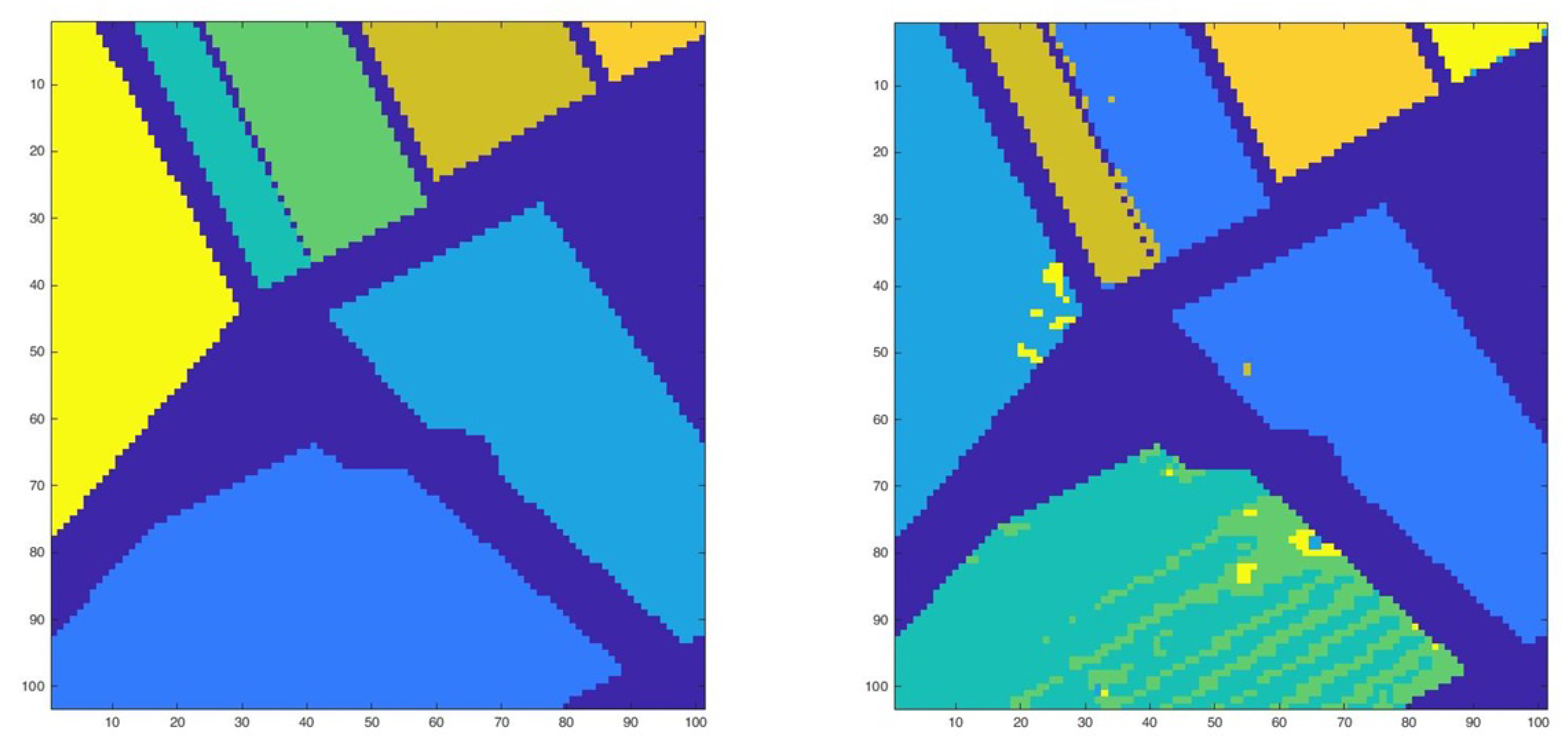
The confusion matrix acquired for Set 1, where an observation known to be in class i was predicted in class j [see Table 1]. As we can see, the table demonstrates a good classification [see Figure 2], except for class 4, which was classified as class 2. Figure 3 shows the output of classification for Set 2.
2.2. K-Means Clustering
The K-means algorithm classifies the data by grouping the items into k different clusters. The results are obtained by using the Euclidean distance [17].
2.3. Parafac Classification
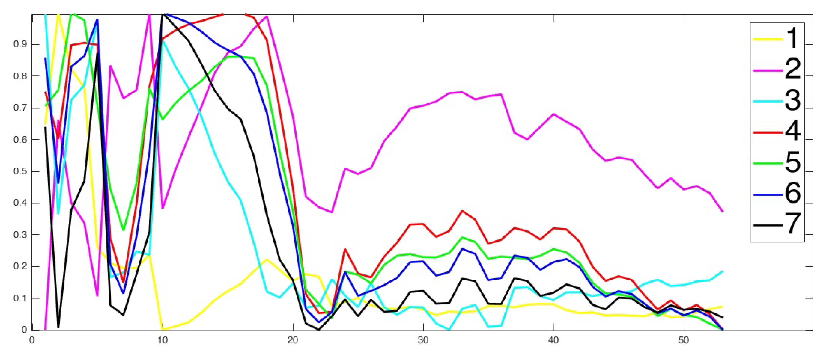
Parallel Factor Analysis (Parafac) is a method to decompose multi-way data and analyze the data using non-supervised classification tools. In Figure 8 are the mean of spectral bands for each class for Danube Delta, Romania (Set 5). The number of Parafac components was 100, the algorithm converged after 2 iterations, and the explained variation was 98.73.
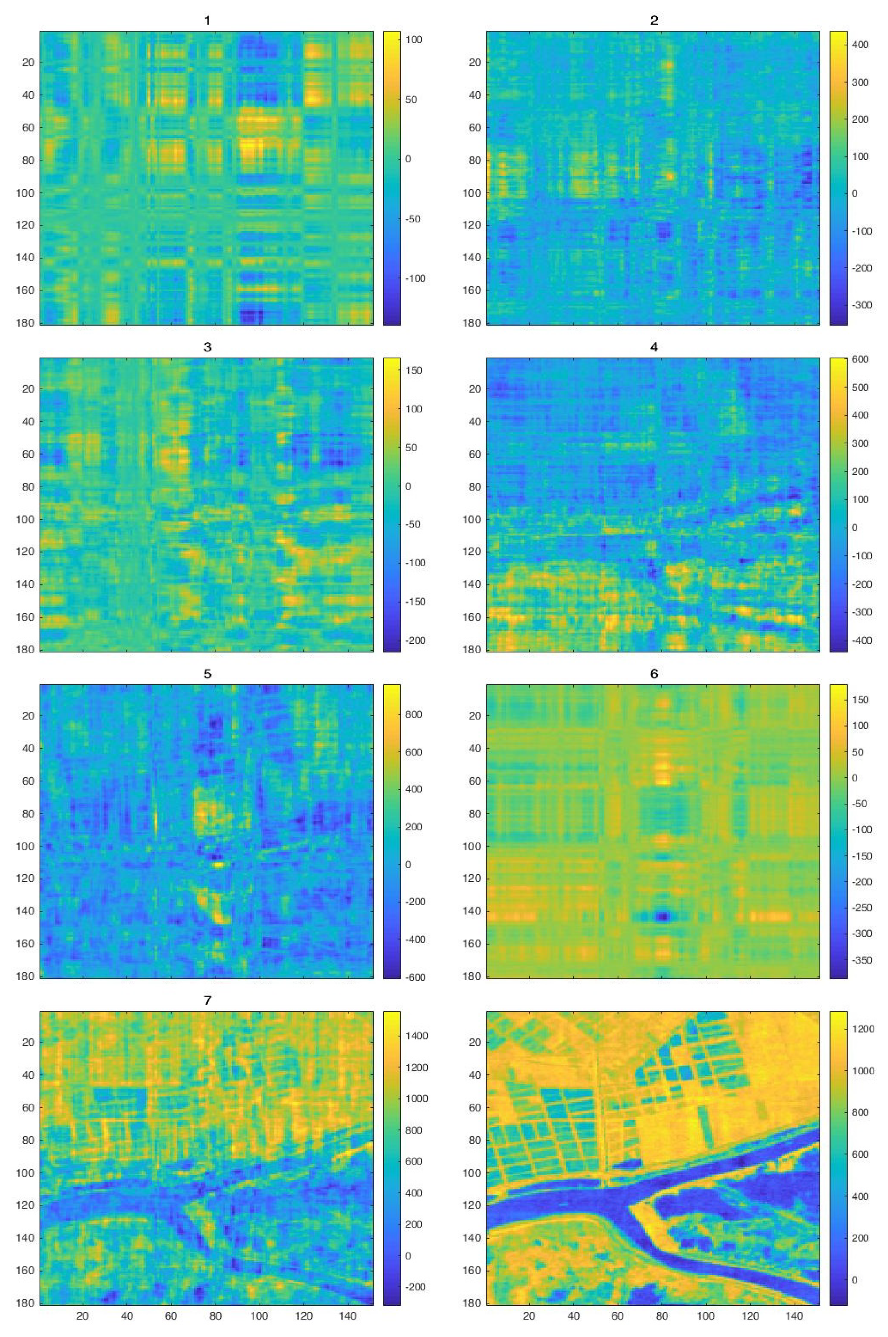
Figure 9 shows the estimated abundance maps for each class, blue for low contribution to yellow to high contribution. Also, we can observe that there are classes which do not distinguish very well and one of the reasons for this could be the poor resolution of the hyperspectral image. On the fourth row in the second image, it can be easily seen that the areas are very well delimited by analyzing Figure 7 (left).
The pseudo-code that describes the construction of an abundance map is presented in Algorithm 1. Figure 9 shows the abundances maps for each class, constructed by using the algorithm described previously. We used the same algorithm for all the data sets we discussed in this paper. In Section 5, we discuss the results presented previously.
| Algorithm 1: The construction of abundance map |
 |
3. Discussion
The results from three classifications methods are summarized in Table 3, Table 4 and Table 5. Because we started with the assumption that the ground truth is unknown, we evaluated the classification using the following measures—Silhouette Coefficient, and Davies-Bouldin Index. Further, we calculated the accuracy and confusion matrix by using the ground truth.
Table 3 and Table 4 contain the evaluation results of classification. The good classification performance is demonstrated by accuracy values which are higher than 84% for both K-means and Hierarchical clustering. We can see that the number of classes from ground truth does not match with the number of classes proposed by the Silhouette score for all data sets. One reason can be the resolution of images and the quality of ground truth. In the case of Set 5—Danube Delta—because the ground truth is missing, we do not have the accuracy value and number of classes.
In Table 5, we have on the line number of sets, and on the column, we have the classes. For each set, we calculated The Root Mean Squared Error between means of spectral bands for each class from ground truth and the means of spectral bands for each class from classification result. In Table 5, we highlighted the pairs with the lowest value of Root Mean Squared Error. Even though we classified the spectral bands in 7 clusters for this data set, the RMSE associate one class resulted from Parafac Decomposition with more than one class from the ground truth [see Table 5].
4. Methods
Regarding the high dimensionality of hyperspectral images, dimension reduction is an important step to process the hyperspectral information. Many techniques were tried to improve the performance of dimension reduction to detect, recognize and classify the materials. Next, we describe the algorithms addressed in this paper.
4.1. Parafac Decomposition
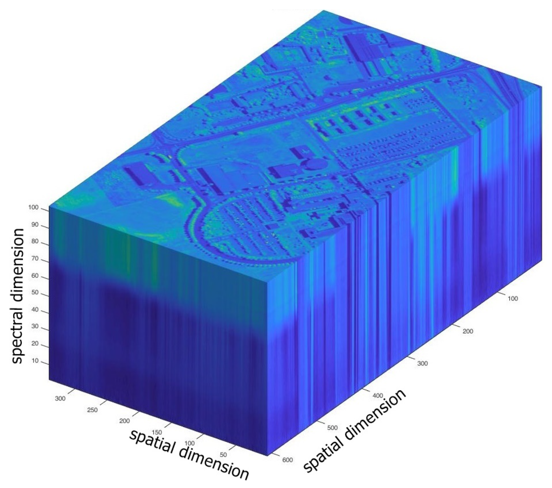
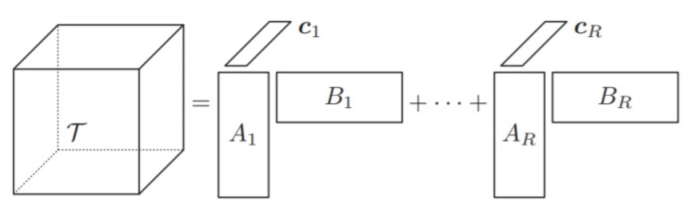
In practice, hyperspectral images are tensors of three-order [see Figure 10]. Give, a hypespectral tensor , is the number of pixels and M is the spectral signature. A tensor is a multidimensional array called order tensor or N-way tensor, where [18].
CANDECOMP/Parafac Decomposition of a higher-order tensor is decomposition in a minimal number of rank-1 tensors [see Equation (1)]. For a third order tensor , the Parafac decomposition is written as [see Figure 11] [12,19]:
In Equation (1), A, B and, C are the loading matrices, R is a positive integer and, the symbol ∘ denotes the outer product of vectors.
Spectral unmixing assumes “the decomposition of the measured spectrum of a mixed pixel into a set of pure spectral signatures (endmembers) and their corresponding abundances (fractional area coverage of each endmember present in the pixel)” [20]. The mixed pixels contain a combination of different materials. In Equation (2) is written the linear mixture model for each pixel:
where is the spectrum of the pixel and L is the number of bands, is a matrix in which each column corresponds to the spectrum of an endmember, P is the number of endmembers, contains the fractional abundances of the endmembers and, e is additive noise [20]. In Equation (3) is written the mixing model for N pixels:
where the matrix contains all pixels from hyperspectral data and contains the fractional abundances of all pixels on all endmembers [21].
Making a connection between Block Term Decomposition, and linear spectral mixture model (LSMM), the previous equation can be seen as a problem of matrix factorization. According to LSMM, it is expected to be the product between a matrix and a vector. The vector contains the endmembers, and the matrix contains the abundances of the corresponding endmember for every pixel, and also the spatial position of pixels [21].
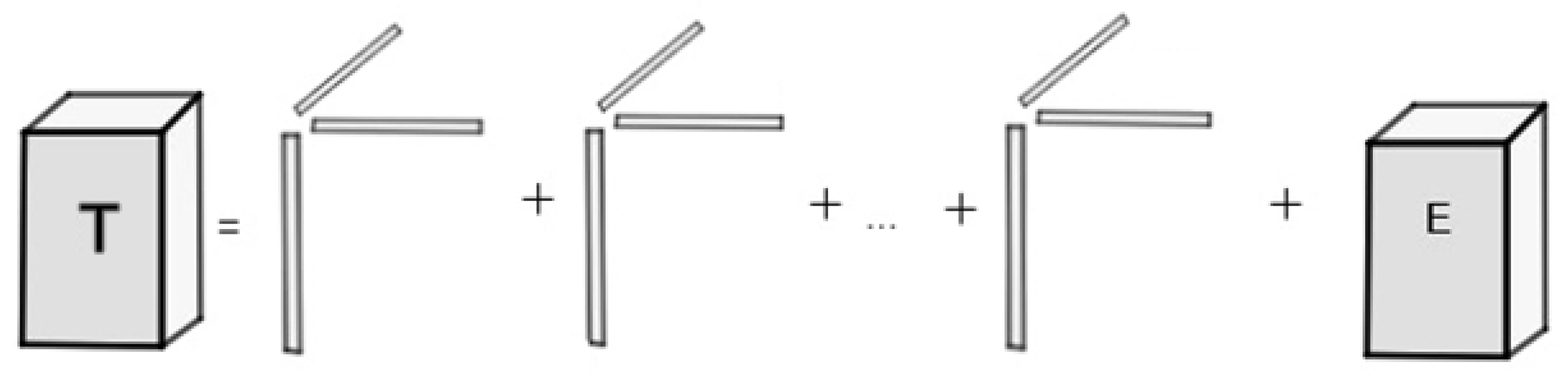
The rank- block term decomposition approximates a tensor of order three in a sum of R terms and, each term is an outer product of rank matrix and, a nonzero vector [see Figure 12]. In Equation (4) is written the rank- BTD of a tensor T [22]:
where are ranks, is called abundance map representing the product and nonzero . Spectral unmixing makes possible a decomposition of a hyperspectral image to obtain the corresponding abundance map [23].
4.2. K-means and Hierarchical Clustering
Hierarchical clustering and K-means are unsupervised classifiers that look for similarities among data and, both use the same approaches to decide the number of clusters [24].
To evaluate the performance of the classification, we used the Davies-Bouldin Index, whose values signify the average similarity between clusters. The similarity is a measure that compares the distance between clusters with the size of the clusters themselves; a value closer to 0 or 0 indicates a better partition. Also, we used the Silhouette Coefficient, where a higher Silhouette Coefficient score indicates better-defined clusters [25]. Using the ground truth, we could calculate the contingency matrix and accuracy value [25].
5. Conclusions
This study has addressed the problem of the classification of hyperspectral images using K-means, Parafac Decomposition, and Hierarchical clustering. The following discussion implies a comparative analysis of three different classification methods for hyperspectral images. The run-time is the total time from when an algorithm starts to its finish [26]. Taking into account this challenge, the execution time depends on many factors, but the most important is the memory used, the percentage of CPU utilized by an algorithm and the data set dimensions. Considering these results, Parafac decomposition is very useful for big data, because it is important to reduce the execution time and to use memory efficiently. According to the results in Section 3, we can say that for small data, K-means or hierarchical classification can be used. For big data, Parafac decomposition can be used because it reduces the data and becomes easy to interpret; the execution time will be considerably reduced. Additionally, the abundance maps are very well defined, considering that the fraction of a pixel class is estimated by an abundance map. In other words, the abundance map could be seen as ground truth, noting that possible errors of human errors of the class assignment are non-existent. Regarding K-means and Hierarchical clustering, we can see that it offered very good accuracy values but, at the same time, we must take into account that, for big data, the execution time will grow considerably.
By comparing the supervised and unsupervised classification, the supervised classification yielded better results, but it forces us to have ground truth [27]. However, the results for unsupervised classification are not so far from supervised classification. The unpleasant results of classification after Parafac decomposition can be caused by spatial and spectral resolution. Finally, the studied algorithms have been shown to be effective for our problems, are very useful in applications such as model reduction, pattern recognition and classification.
Author Contributions
The authors contributed equally to this work. All authors have read and agreed to the published version of the manuscript.
Funding
This work was supported by the project ANTREPRENORDOC, in the framework of Human Resources Development Operational Programme 2014-2020, financed from the European Social Fund under the contract number 36355/23.05.2019 HRD OP/380/6/13–SMIS Code: 123847.
Conflicts of Interest
The authors declare no conflict of interest.
References
- Audebert, N.; Saux, B.; Lefèvre, S. Deep Learning for Classification of Hyperspectral Data: A Comparative Review. IEEE Geosci. Remote Sens. Mag. 2019, 7. [Google Scholar] [CrossRef] [Green Version]
- Wang, D.; Cheng, B. An Unsupervised Classification Method of Remote Sensing Images Based on Ant Colony Optimization Algorithm. In Advanced Data Mining and Applications; Cao, L., Feng, Y., Zhong, J., Eds.; Springer: Berlin/Heidelberg, Germany, 2010; pp. 294–301. [Google Scholar]
- Wu, M.; Wei, D.Z.L.Z.Y. Hyperspectral Face Recognition with Patch-Based Low Rank Tensor Decomposition and PFFT Algorithm. Symmetry 2018, 10, 714. [Google Scholar] [CrossRef] [Green Version]
- Ganci, G.; Vicari, A.; Fortuna, L.; Negro, C.D. The HOTSAT volcano monitoring system based on combined use of SEVIRI and MODIS multispectral data. Ann. Geophys. 2011, 54. [Google Scholar] [CrossRef]
- Zhou, D.; Xiao, J.; Bonafoni, S.; Berger, C.; Deilami, K.; Zhou, Y.; Frolking, S.; Yao, R.; Qiao, Z.; Sobrino, J. Satellite Remote Sensing of Surface Urban Heat Islands: Progress, Challenges, and Perspectives. Remote Sens. 2018, 11, 48. [Google Scholar] [CrossRef] [Green Version]
- Sahar, A. Hyperspectral Image Classification Using Unsupervised Algorithms. Int. J. Adv. Comput. Sci. Appl. 2016, 7. [Google Scholar] [CrossRef] [Green Version]
- Moughal, T.A. Hyperspectral image classification using Support Vector Machine. J. Phys. Conf. Ser. 2013, 439, 012042. [Google Scholar] [CrossRef]
- Hosseini, L.; Kandovan, R. Hyperspectral Image Classification Based on Hierarchical SVM Algorithm for Improving Overall Accuracy. Adv. Remote Sens. 2017, 6, 66–75. [Google Scholar] [CrossRef] [Green Version]
- Senapati, S. Unsupervised Classification of Hyperspectral Images Based on Spectral Features. Bacherlor’s Thesis, Department of Electronics and Communication Engineering, National Institute of Technology Rourkela, Rourkela, India, 2015. [Google Scholar]
- Ranjan, S.; Nayak, D.; Kumar, S.; Dash, R.; Majhi, B. Hyperspectral image classification: A k-means clustering based approach. In Proceedings of the 2017 4th International Conference on Advanced Computing and Communication Systems (ICACCS) 2017, Coimbatore, India, 6–7 January 2017; pp. 1–7. [Google Scholar] [CrossRef]
- Veganzones, M.A.; Cohen, J.; Farias, R.C.; Marrero, R.; Chanussot, J.; Comon, P. Multilinear spectral unmixing of hyperspectral multiangle images. In Proceedings of the 2015 23rd European Signal Processing Conference (EUSIPCO), Nice, France, 31 August –4 September 2015; pp. 744–748. [Google Scholar]
- Phan, A.H.; Cichocki, A. Tensor decompositions for feature extraction and classification of high dimensional datasets. Nonlinear Theory Its Appl. IEICE 2010, 1, 37–68. [Google Scholar] [CrossRef] [Green Version]
- Arena, P.; Bucolo, M.; Fazzino, S.; Fortuna, L.; Frasca, M. The CNN Paradigm: Shapes and Complexity. Int. J. Bifurc. Chaos 2005, 15, 2063–2090. [Google Scholar] [CrossRef]
- GIC. Grupo de Inteligencia Computacional Hyperspectral Remote Sensing Scenes. Available online: http://www.ehu.eus/ (accessed on 1 September 2019).
- USGS. Earthexplorer.usgs.gov, U.S. Geological Survey. Available online: https://earthexplorer.usgs.gov (accessed on 1 September 2019).
- Christian, E.; Jiman, H.; Kim-Kwang, C. Pervasive Systems, Algorithms and Networks. In Proceedings of the 16th International Symposium (I-SPAN 2019), Naples, Italy, 16–20 September 2019. [Google Scholar] [CrossRef]
- GeeksforGeeks. A Computer Science Portal for Geeks, GeeksforGeeks. Available online: https://www.geeksforgeeks.org/ (accessed on 1 September 2019).
- Tamara Kolda, B.W. Tensor Decompositions and Applications. Soc. Ind. Appl. Math. 2009, 51, 455–500. [Google Scholar]
- Ignat Domanov, L.L. On the uniqueness of the canonical polyadic decomposition of third-order tensors-Part II: Uniqueness of the overall decomposition. SIAM J. Matrix Anal. Appl. 2013, 34, 876–903. [Google Scholar]
- Chen Shi, L.W. Linear Spatial Spectral Mixture Model. IEEE Trans. Geosci. Remote. Sens. 2016, 54, 3599–3611. [Google Scholar]
- Yuntao, Q.; Fengchao, X. Matrix-Vector Nonnegative Tensor Factorization for Blind Unmixing of Hyperspectral Imagery. IEEE Trans. Geosci. Remote Sens. 2017, 55, 1776–1792. [Google Scholar]
- Sorber, L.; Barel, M.V.; Lathauwer, L.D. Optimization-Based Algorithms for Tensor Decompositions: Canonical Polyadic Decomposition, Decomposition in Rank-(Lr,Lr,1) Terms And A New Generalization. SIAM J. Optim. 2013, 23, 695–720. [Google Scholar] [CrossRef] [Green Version]
- Veganzones, M.; Cohen, J. Canonical Polyadic Decomposition of Hyperspectral Patch Tensors. In Proceedings of the 2016 24th European Signal Processing Conference (EUSIPCO), Budapest, Hungary, 28 August–2 September 2016; pp. 2176–2180. [Google Scholar] [CrossRef] [Green Version]
- Nielsen, F. Hierarchical Clustering. In Introduction to HPC with MPI for Data Science; Springer: Berlin, Germany, 2016; pp. 195–211. ISBN 978-3-319-21902-8. [Google Scholar] [CrossRef]
- Scikit-Learn. Scikit-learn, Learn: Machine Learning in Python—Scikit-Learn 0.16.1 Documentation. Available online: https://scikit-learn.org/ (accessed on 1 November 2019).
- Doan, T.; Kalita, J. Predicting run time of classification algorithms using meta-learning. Int. J. Mach. Learn. Cybern. 2016, 8. [Google Scholar] [CrossRef]
- Bilius, L.B.; Pentiuc, S.G.; Brie, D.; Miron, S. Analysis of hyperspectral images using supervised learning techniques. In Proceedings of the 23rd International Conference on System Theory, Control and Computing, ICSTCC, Sinaia, Romania, 9–11 October 2019. [Google Scholar] [CrossRef]
Figure 1.
Remote sensing [5].
Figure 1.
Remote sensing [5].

Figure 2.
Ground Truth (left) and Hierarchical classification for Set 1 (right).

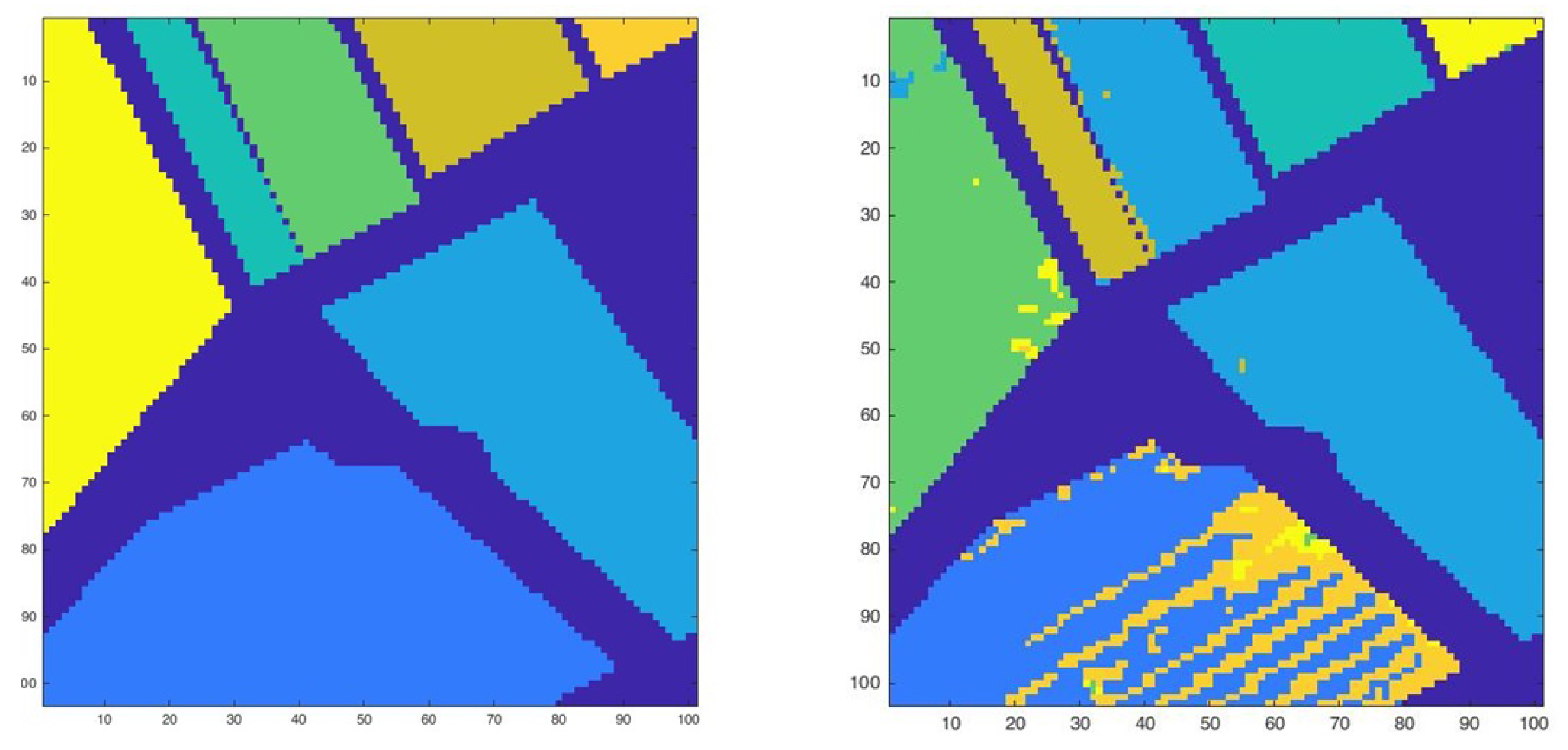
Figure 3.
Ground Truth (left) and Hierarchical classification for Set 2 (right).

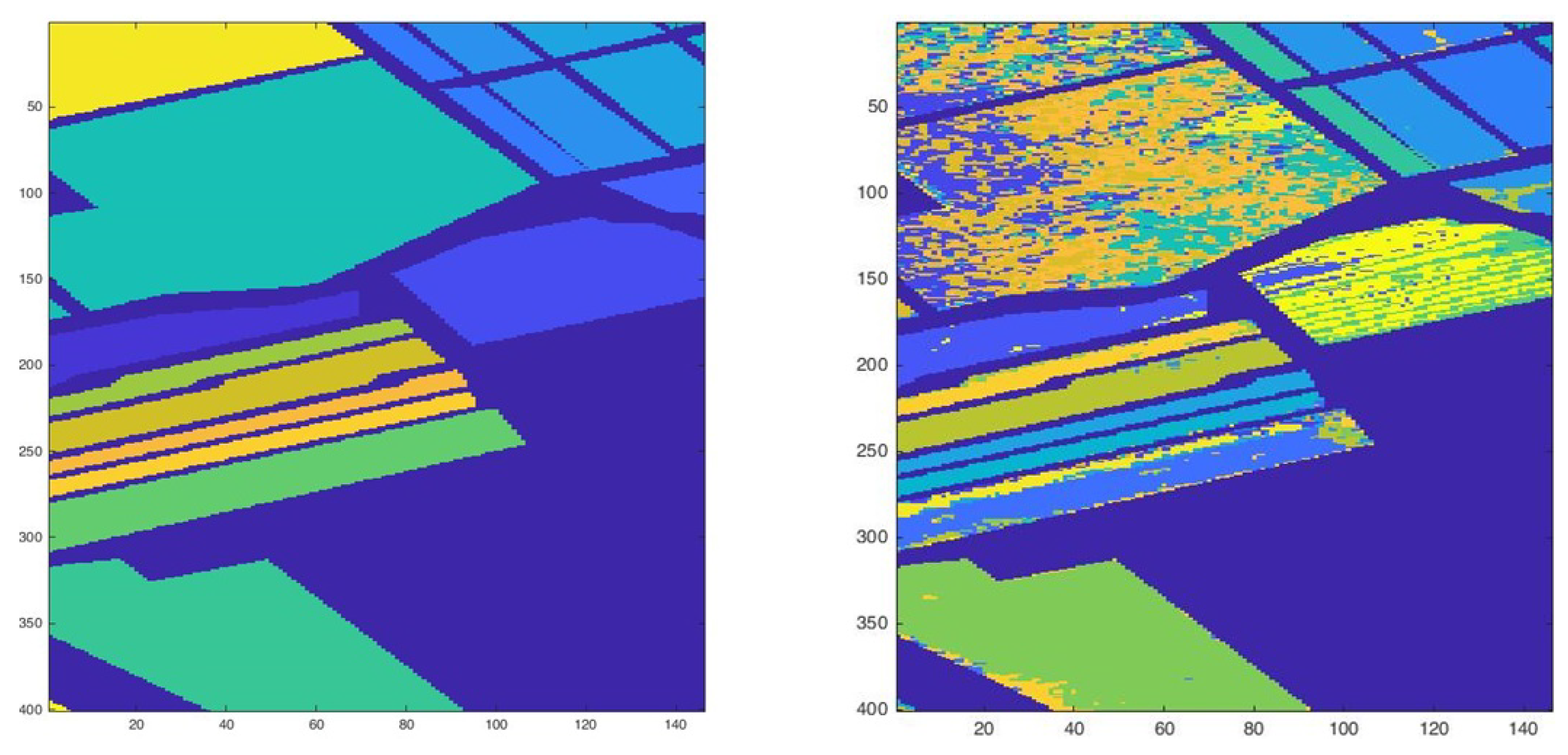
Figure 4.
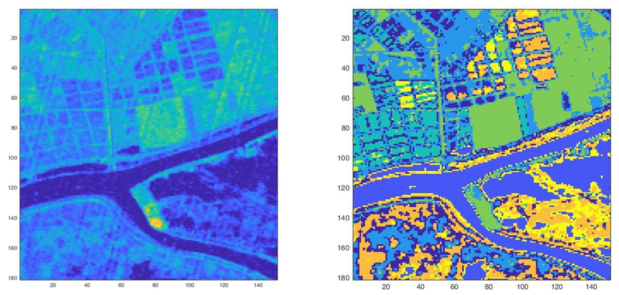
Original hyperspectral image (left) and Hierarchical classification for Set 5 (right).

Figure 5.
Ground Truth (left) and K-means classification for Set 1 (right).

Figure 6.
Ground Truth (left) and K-means classification for Set 2 (right).

Figure 7.
Original hyperspectral image (left) and K-means classification for Set 5 (right).

Figure 8.
The mean of Spectral bands after Parafac Decomposition.

Figure 9.
The abundance map of Danube Delta.

Figure 10.
Hyperspectral image tensor.

Figure 11.
The Parafac decomposition of a three order tensor [18].
Figure 11.
The Parafac decomposition of a three order tensor [18].

Figure 12.
Rank- block term decomposition of a third order tensor [22].
Figure 12.
Rank- block term decomposition of a third order tensor [22].


Table 1.
Confusion Matrix of Set 1 after Hierarchical classification.
| 1 | 2 | 3 | 4 | 5 | 6 | 7 | Total | |
|---|---|---|---|---|---|---|---|---|
| 1 | 2291 | 0 | 0 | 0 | 0 | 29 | 6 | 2326 |
| 2 | 0 | 1772 | 2 | 0 | 0 | 0 | 0 | 1774 |
| 3 | 0 | 2 | 362 | 0 | 0 | 0 | 0 | 364 |
| 4 | 0 | 657 | 25 | 0 | 0 | 0 | 0 | 682 |
| 5 | 0 | 0 | 0 | 0 | 539 | 0 | 0 | 539 |
| 6 | 0 | 0 | 0 | 0 | 0 | 98 | 4 | 102 |
| 7 | 0 | 0 | 0 | 0 | 0 | 24 | 1258 | 1282 |
| % | 98.49 | 99.88 | 99.45 | 0 | 100 | 96.07 | 98.12 |
1—broccoli green weeds 2; 2—fallow; 3—fallow rough plow; 4—fallow smooth; 5—stubble; 6—celery; 7—grapes untrained.
Table 2.
Confusion Matrix of Set 1 after K-means classification.
| 1 | 2 | 3 | 4 | 5 | 6 | 7 | Total | |
|---|---|---|---|---|---|---|---|---|
| 1 | 2280 | 0 | 0 | 0 | 0 | 41 | 5 | 2326 |
| 2 | 0 | 1772 | 2 | 0 | 0 | 0 | 0 | 1774 |
| 3 | 0 | 2 | 362 | 0 | 0 | 0 | 0 | 364 |
| 4 | 0 | 656 | 26 | 0 | 0 | 0 | 0 | 682 |
| 5 | 0 | 1 | 0 | 0 | 538 | 0 | 0 | 539 |
| 6 | 0 | 0 | 0 | 0 | 0 | 100 | 2 | 102 |
| 7 | 2 | 16 | 0 | 0 | 0 | 29 | 1235 | 1282 |
| % | 98.02 | 99.88 | 99.45 | 0 | 99.81 | 98.03 | 96.33 |
1—broccoli green weeds 2; 2—fallow; 3—fallow rough plow; 4—fallow smooth; 5—stubble; 6—celery; 7—grapes untrained.
Table 3.
Results of Hierarchical clustering.
| Set | Sil. Score 1 | DB 2 | Exe. 3 | Acc. 4 | Cl. 5 |
|---|---|---|---|---|---|
| 1 | 0.701(7) | 0.400 | 0.020 | 0.894 | 7 |
| 2 | 0.427(16) | 0.731 | 0.094 | 0.847 | 16 |
| 3 | 0.539(11) | 0.586 | 0.012 | 0.961 | 6 |
| 4 | 0.802 (6) | 0.568 | 0.027 | 0.946 | 6 |
| 5 | 0.260 (7) | 1.288 | 0.058 | - | - |
1 Maximum value of Silhouette scores calculated, and the number of classes used, 2 Davies-Bouldin Index, 3 The execution time of classification expressed in seconds (s), 4 Accuracy (using ground truth), 5 Number of classes from ground truth.
Table 4.
Results after K-means classification.
| Set | Sil. Score 1 | DB 2 | Exe. 3 | Acc. 4 | Cl. 5 |
|---|---|---|---|---|---|
| 1 | 0.700(7) | 0.411 | 1.925 | 0.889 | 7 |
| 2 | 0.4462(17) | 0.711 | 19.963 | 0.847 | 16 |
| 3 | 0.575(10) | 0.520 | 0.707 | 0.969 | 6 |
| 4 | 0.806(6) | 0.550 | 0.877 | 0.950 | 6 |
| 5 | 0.309(7) | 1.154 | 3.854 | - | - |
1 Maximum value of Silhouette scores calculated, and the number of classes used, 2 Davies-Bouldin Index, 3 The execution time of classification expressed in seconds (s), 4 Accuracy (using ground truth), 5 Number of classes from ground truth.
Table 5.
Comparison of run time between K-means, Hierarchical clustering and Classification after using Parafac decomposition and results after Parafac Classification.
Table 5.
Comparison of run time between K-means, Hierarchical clustering and Classification after using Parafac decomposition and results after Parafac Classification.
| Set | 1 | 2 | 3 | 4 | 5 |
|---|---|---|---|---|---|
| Execution Time | |||||
| Parafac 1 | 4.23 | 12.03 | 3.63 | 4.27 | 3.25 |
| Classification 2 | 5975 | 2880 | 2363 | 3603 | 1498 |
| Class. K-means 3 | 0.030 | 36.47 | 0.048 | 0.069 | 0.059 |
| Class. Hierarchical 4 | 2.448 | 3794 | 3.954 | 5.290 | 3.855 |
| Class | Class Distribution | ||||
| 1 | 6 | 14 | 4 | 5 | - |
| 2 | 5 | 5 | 3 | 2 | - |
| 3 | 6 | 16 | 4 | 1 | - |
| 4 | 4 | 5 | 1 | 2 | - |
| 5 | 7 | 1 | 3 | 2 | - |
| 6 | 6 | 8 | 5 | 3 | - |
| 7 | 4 | 14 | - | - | - |
| 8 | - | 1 | - | - | - |
| 9 | - | 7 | - | - | - |
| 10 | - | 16 | - | - | - |
| 11 | - | 5 | - | - | - |
| 12 | - | 6 | - | - | - |
| 13 | - | 16 | - | - | - |
| 14 | - | 9 | - | - | - |
| 15 | - | 7 | - | - | - |
| 16 | - | 14 | - | - | - |
1 The execution time expressed in seconds (s), 2. The execution time expressed in microseconds (), 3 The execution time expressed in seconds (s) using K-means for the entire data set, 4 The execution time expressed in seconds (s) using Hierarchical clustering for the entire data set.
© 2020 by the authors. Licensee MDPI, Basel, Switzerland. This article is an open access article distributed under the terms and conditions of the Creative Commons Attribution (CC BY) license (http://creativecommons.org/licenses/by/4.0/).
Share and Cite
MDPI and ACS Style
Bilius, L.B.; Pentiuc, S.G. Unsupervised Clustering for Hyperspectral Images. Symmetry 2020, 12, 277. https://doi.org/10.3390/sym12020277
AMA Style
Bilius LB, Pentiuc SG. Unsupervised Clustering for Hyperspectral Images. Symmetry. 2020; 12(2):277. https://doi.org/10.3390/sym12020277
Chicago/Turabian StyleBilius, Laura Bianca, and Stefan Gheorghe Pentiuc. 2020. "Unsupervised Clustering for Hyperspectral Images" Symmetry 12, no. 2: 277. https://doi.org/10.3390/sym12020277
Note that from the first issue of 2016, this journal uses article numbers instead of page numbers. See further details here.