Article

Predicting Daily Air Pollution Index Based on Fuzzy Time Series Markov Chain Model

by
Yousif Alyousifi
1,*,
Mahmod Othman
1,
Rajalingam Sokkalingam
1,
Ibrahima Faye
2 and
Petronio C. L. Silva
3
1
Fundamental and Applied Sciences Department, Universiti Teknologi PETRONAS, Seri Iskandar 32160, Malaysia
2
Center for Intelligent Signal and Imaging Research & Fundamental and Applied Sciences Department, Universiti Teknologi PETRONAS, Seri Iskandar 32160, Malaysia
3
Instituto Federal do Norte de Minas – IFNMG, Januária 39400-149, Brazil
*
Author to whom correspondence should be addressed.
Symmetry 2020, 12(2), 293; https://doi.org/10.3390/sym12020293
Submission received: 15 January 2020 / Revised: 10 February 2020 / Accepted: 11 February 2020 / Published: 17 February 2020

Abstract

:
Air pollution is a worldwide problem faced by most countries across the world. Prediction of air pollution is crucial in air quality research since it is related to public health effects. The symmetry concept of fuzzy data transformation from a single point (crisp) to a fuzzy number is essential for the forecasting model. Fuzzy time series (FTS) is applied for predicting air pollution; however, it has a limitation caused by utilizing an arbitrary number of intervals. This study involves predicting the daily air pollution index using the FTS Markov chain (FTSMC) model based on a grid method with an optimal number of partitions, which can greatly develop the model accuracy for air pollution. The air pollution index (API) data, which was collected from Klang, Malaysia, is considered in the analysis. The model has been validated using three statistical criteria, which are the root mean (RMSE), the mean absolute percentage error (MAPE), and the Thiels’ U statistic. Also, the model’s validation has been investigated by comparison with some of the famous statistical models. The results of the proposed model demonstrated outperformed the other models. Thus, the proposed model could be a better option in air pollution forecasting that can be useful for managing air quality.

1. Introduction

Air pollution is a matter of concern among the public, particularly for those who live in mega-urban and industrial cities, which may have serious effects on humans and the natural environment in the future [1]. Air pollution forecasting is a high-priority in air quality research since it is related to public health effects and the natural environment [2,3,4]. The most widely important classical methods of time series are the autoregressive integrated moving average (ARIMA) models [5], the artificial neuron network (ANN) models [6,7,8], and the fuzzy time series (FTS) [9,10,11,12,13,14,15,16,17].
The FTS model is first introduced by Song and Chissom [18,19] based on a fuzzy set theory proposed by Zadeh [20]. Chen [21] developed the FTS model of Song and Chissom based on fuzzy logic group relations tables for reducing the computational complexity in the model. Huarng [22,23] developed Chen’s [21] model by determining the effective length of intervals. Yolcu et al. [24] developed the ratio-based method based on a constrained optimization to select the length of intervals. Yu [25] improved a predicting model based on weighted fuzzy relations, which produced better forecasting results than the Chen [21] model. Cheng et al. [26] introduced the trend weighted FTS model for TAIEX forecasting by assign proper weights to individual fuzzy relationships. Effindy et al. [27] modified a weighted FTS model for enrollment forecasting. They adopted the weighted model by adding the difference between the observed dataset across a midpoint of intervals. Tsaur [28] proposed the FTS model based on Markov chain, which is used for obtaining the largest probability using the transition probability matrix. He also used a random length of interval for the universe of discourse, which leads to a negative effect by abnormal observations and outliers. Sadaei et al. [29] developed a refined exponentially weighted FTS for forecasting the load data, which is developed prediction preciseness. More specifically, the effective interval length has been investigated by several studies based on different methods. For example, Huarng [22,23] proposed two methods for determining the effective length of intervals, which are based on averages and distribution. Yolcu et al. [24] developed Huarng’s model [22] based on constrained optimization for determining the effective length of intervals. Eğrioğlu et al. [30] proposed a new method of fuzzy time series using a single variable constrained optimization to determine the best length of interval for the best forecasting accuracy. Chen et al. [31] proposed a new FTS forecasting model integrated with the granular computing approach and entropy method for stock price data. Talarposhti et al. [32] proposed a hybrid approach using optimization techniques and intelligence algorithm to determine the proper length of intervals for predicting the stock market. Cheng et al. [33] employed a rough set and utilized an adaptive expectation model to propose a new fuzzy time series to forecast the closing price. Rahim et al. [34] developed a type 2 FTS model using the sliding window technique for determining the appropriate length of intervals. Bose et al. [35] proposed a new partitioning method with the rough-fuzzy method for developing the fuzzy time series model.
Apart from that, Zuo et al. [36] developed a combining topological optimization technique in order to figure out the optimization problem in the product manufacturing process. Ning et al. [37] proposed a new method based on a chip formation model and an iterative gradient search method using Kalman filter algorithm. This optimization method has been used to inversely identify the Johnson-Cook model constants of ultra-fine-grained titanium. Ning and Liang [38] introduced a developed inverse identification technique for Johnson-Cook model constants based on the use of temperature and force data for predicting machining forces. The development of the model has been done by using an iterative gradient search method based on the Kalman filter algorithm. These types of optimization techniques can be adopted for improving the forecasting models.
More specifically, The FTS models have been utilized for forecasting environmental problems such as air quality 9-17], which are considered for predicting air pollution since the time series of air pollution may include uncertainty data and may not verify some of the statistical assumptions. Nevertheless, utilizing the FTS models in the field of air pollution is still very rare. For example, Cheng et al. [17] introduced a trend weighted FTS model to predict daily O3 concentrations. Dincer and Akkuş [12] predicted the SO2 concentrations based on a robust FTS model, which has provided good forecasting results. Koo et al. [39] made a comparison study using FTS and other statistical models for predicting air pollution events. They concluded that the proposed model outperformed the other models. Wang et al. [40] proposed a hybrid FTS method with data re-processing approaches for forecasting the main air pollutants. Yang et al. [41] proposed a forecasting system based on a combination of the fuzzy theory and advanced optimization algorithm for air pollution forecasting.
As previously mentioned, the FTS models have been utilized to solve various domain forecasting problems. However, several FTS have some issues, such as using an arbitrary length of intervals for the universe of discourse, repeated fuzzy relationships, or considering the weights of fuzzy logical relationships. According to the literature review above, some researchers proposed a partition method with complexity computations, and some have not evaluated their models, by comparison with the other recent models. Particularly, the FTS-based Markov chain model has a deficiency in determining the effective length of the interval, which was negatively affected by abnormal observations and outliers. Therefore, determining the optimal length of intervals and assigning the proper weights to present is an interesting issue that needs to be addressed. This motivated us to investigate the optimal partition number of the universe of discourse. This study proposes the FTS Markov chain (FTSMC) model based on the grid method with the optimal number of the partitions of the universe of discourse to provide significantly improved performance in the model accuracy for air pollution forecasting. The major contribution of this study is to propose an improved model with an appropriate partition number and to implement the model for forecasting APIs as a new forecasting model in air quality research.

2. Preliminary

Fuzzy Time-Series Definitions

The fundamental steps for designing fuzzy time series models are defined universe of discourse U , divide U into an equal number of intervals, fuzzification, define fuzzy logic relation, determined forecasted values, and defuzzification. The main time series definitions of developed are listed below:
Definition 1.
Let X ( t ) ( t   = 0 ,   1 ,   2 ,   .   .   . ) , a subset of real numbers, be the universe of discourse in which fuzzy sets f j ( t ) are defined. Let F ( t ) be a collection of f 1 ( t ) ,   f 2 ( t ) , …, then F ( t ) is called a fuzzy time series, defined on X ( t ) [17,18,19].
Definition 2.
Let R ( t ,   t   1 ) be the fuzzy logic relationship (FLR) between F ( t 1 ) and F ( t ) , which can be denoted as F ( t 1 )   F ( t ) . For anytvalue, if R ( t ,   t   1 ) is independent of t, then
R ( t ,   t   1 ) =   R ( t 1 ,   t   2 )
In this case, F ( t ) is called the time-invariant fuzzy time series, while otherwise called a time-variant fuzzy time series [18,19].
Definition 3.
Suppose that F ( t 1 ) = A i and the F ( t ) = A j . The relationship between two consecutive observations ( t 1 ) and F ( t ) , denoted to as the FLR can be defined as A i A j , where A i and A j are the left-hand side and right-hand side of the FLR respectively [17,18,19].

3. Methodology

3.1. Study Area and Dataset

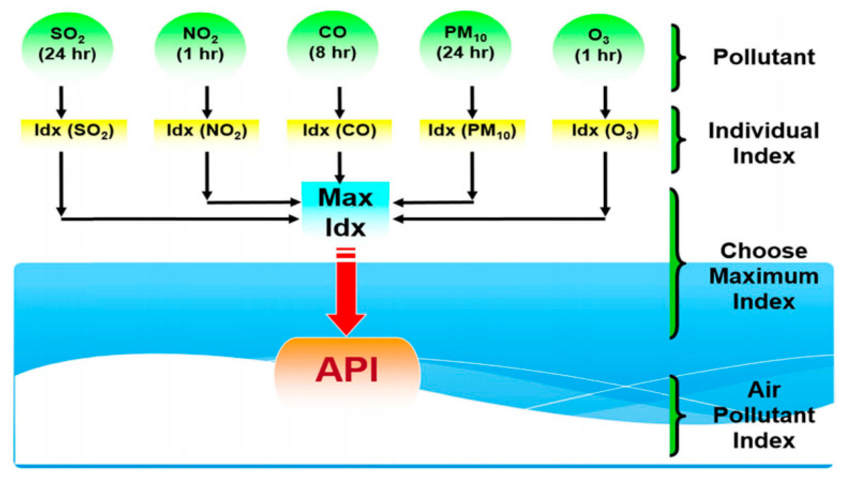
The air pollution index (API) data is classified based on the highest index value of five main air pollutants, namely, ozone (O3), sulphur dioxide (SO2), particulate matter (PM10), carbon monoxide (CO2), and nitrogen dioxide (NO2), as shown in Figure 1 [42,43,44,45]. The API values are determined by the average indices for these five pollutant variables, and then the maximum value from these sub-indices is selected as the API value [3]. In Malaysia, the air pollution index (API) has been adopted as a measure of air pollution conditions. The API is a simple number that ranges from 0 to ∞ to reflect the air quality levels that are related to the health effects [3,45].
In this study, the daily API maxima values, which were gathered from an air monitoring station located in Klang, Malaysia, are considered in the analysis. The city of Klang is located nearly 32 km to the west side of Kuala Lumpur and covers a land area of about 573 km2, as shown in Figure 2. The API dataset is divided into a training dataset, which is from the 1 January 2012 to 31 December 2013 and testing dataset, which is from the1 January 2014 to 31 December 2014. The values of API recorded at the selected monitoring station are provided by the Department of Environment of Malaysia. The total number of observations in this study is 1096. The value of API of less than 100 denotes a good air quality, while a of API greater than 100 indicates a higher degree of air pollution. The classification of states is made based on the breakpoints for API of 50, 100, 200, 300, and 300+, corresponding to good, moderate, unhealthy, very unhealthy, and hazardous states, respectively, as shown in Table 1 [3,45].

3.2. Proposed Model

In this section, the simplified arithmetic operations proposed by Chen [21] and Tsaur [28] are used in the proposed algorithm (see Figure 3). The steps of the proposed model can be described as follows:
Step 1.
Define the universe of discourse ( U ) from the available time-series data, by using the formula U   =   [ D m i n   D 1 ,   D m a x +   D 2 ] , where D m i n and D m a x denote the minimum and the maximum value in the universe of discourse U respectively, D 1 and D 2 represent positive values.
Step 2.
Partition U for the observed data using the grid partition method [21,29] based on a different number of partitions, which are 5, 6, 7, 8, …, 50. But to avoid the redundancy, we present only 5, 10, 15, 20, 25, 30, 35, 40, and 45 numbers of partitions to determine the optimal partition number of partitions of the universe that can improve the model accuracy.
Step 3.
Define the fuzzy sets Ai on U using the following equation
A i = f A i ( u 1 ) u 1 + f A i ( u 2 ) u 2 + + f A i ( u n ) u n
where f A i is the membership function of fuzzy set A i ; f A i : U [ 0 , 1 ] . f A i ( u r ) [ 0 , 1 ] and 1 r n .
Step 4.
Fuzzify the observations into fuzzy numbers based on the maximum membership value.
Step 5.
Construct the fuzzy logical relationships (FLRs) and establish fuzzy logical relation groups (FLRGs) to build frequencies (count) matrix of fuzzy relation between observations.
Step 6.
Generate the Markov weights (transition probability matrix) based on the frequencies of the established (FLRGs) in Step 5. The total number of states is n according to the total number of fuzzy sets. Thus, the matrix P   is P n × n . State transition probability P i j , from state A i to state A j . In other words, P i j is the probability of observing y t + 1 given y t , i.e., P i j = P r ( y t + 1 = j |   y t = i ) , which can be calculated as follows
P i j = N i j N i .   , i , j = 1 , 2 , , n
where N i j is the number of transitions from state A i to state A j , and N i . is the total number of transitions in state A i . The transition probability matrix P is given as
P = [ p 11 p 21 p 12 p 22 p 1 n p 2 n p n 1 p n 2 p n n ]
where P i j ≥ 0 and j = 1 n P i j = 1.
Step 7.
Calculate the forecasted values. The following rules are considered in calculating the forecasts.
Rule 1. In the case of the fuzzy logical relationship group of A i   is one-to-one, in which there only one transition for A i (i.e., A i   A k , with P i k = 1 and   P i j = 0, j k), then the forecasting of F ( t ) is m k , the midpoint of u k , k = 1 , 2 , n , which can be calculated according to Equation (5) below
F   ( t + 1 ) =   m k   P i k   =   m k
Rule 2. In the case of the fuzzy logical relationship group of A i is one-to-many, in which there are more than one transition for A i (i.e., A i   A 1 ,   A 2 ,   .   .   . A n , i   =   1 ,   2 ,   .   .   ,   n ) . Thus, if the state is A i for the actual value Y ( t ) at time t , the forecasted value F ( t + 1 ) can be determined by using Equation (6) below
F   ( t + 1 ) =   m 1 p i 1 + m 1 p 12 + + m i 1 p i ( i 1 ) + Y ( t )   p i i + m i + 1 p i ( i + 1 ) + +   m n p i n
where m 1 ,   m 2 ,   , m n   are the midpoint of u 1 ,   u 2 ,   ,   u n   and m i   is replaced by Y ( t ) for having information further from the state A i at time t.
Step 8.
Adjust the forecasted values by adding the differences of actual values Y ( t ) , which can adjust the forecasted values to reduce the estimated error. The adjusted forecasted values can be written by
F ^   ( t + 1 ) = F   ( t + 1 ) +   diff   ( Y ( t ) )
Step 9.
Validate the model.

3.3. Model Validation

The statistical criteria used to evaluate models are MAPE, RMSE, and Thiels’ U statistic, which are defined in Equations (8)–(10), respectively, where Y i means the real data, F i the forecasted values, and N is the total number of observations. The universe of discourse U is partitioned based on the grid method. The model is trained and tested for 5, 10, 15, 20, 25, 30, 35, and 40 number of partitions, and the results are shown in the next section.
  MAPE   = 1 N i = 1 N | Y i F i Y i | × 100  
  RMSE   = i = 1 N ( Y i F i ) 2 N  
  Theil s     U =   i = 1 N ( Y i F i ) 2       i = 1 N Y i 2   +   i = 1 N F i 2      

4. The Implementation of the Algorithm

In this section, we will provide a result of the proposed model using the daily API data, whose plots for training data and testing data are given in Figure 4, respectively.
The implementation of the proposed model’s algorithm can be done based on pyFTS [46] as follows:
Step 1.
Define U for the APIs values. U = [ D m i n D 1 ,   D m a x + D 2 ]
U = [ 25 5 ,   495 + 5 ] U = [ 20 ,   500 ]
Step 2.
Partitioning U based on different numbers of partitions from 1 to 50. However, to prevent the redundancy where it will be too long, we have only mentioned numbers 5, 10, 15, …, 30 to present the partitioning as shown in Figure 5.
Step 3.
Fuzzy sets are defined. Fuzzy sets A k are determined based on the intervals u k   that already have formed using the grid method in the previous step with the function membership. Then, the fuzzy sets A k can be written as follows using Equation (2). Table 1 reveals the fuzzy sets   A i , ( i = 1 ,   2 ,   ,   n ). The greater the value of i   indicates that the fuzzy set of API values will move from the lowest to the highest fuzzy set of API values.
Step 4.
Transform APIs values into fizzy numbers and find the fuzzy logic relationships (FLRs), as shown in Table 2.
Table 3 reveals the actual API values that have been transferred to the FTS values. Then, the FLRs of these values are determined. Since u 1   has the maximum membership degree in fuzzy set A 0 , observation 51 is transferred to a fuzzy set A 0 . Similarly, the API values have been fuzzified.
Step 5.
Fuzzy logical relationships (FLRs) are determined, and frequencies (count) matrix of fuzzy relation between observations are determined. This step shows the FLRGs can be grouped into the fuzzy logic relationship groups (FLRGs).
It can be seen from Table 4 that thirteen groups of the FTS values are presented, which is found with several FLRs. From Table 4, transition frequency matrix or frequencies (count) matrix of fuzzy relation between observations can be determined, which could be a matrix N 30 × 30 .
Step 6.
Assign the Markov weights based on the matrix of frequencies from Step 5 by using Equation (4), as shown in Table 4. Then, transition process diagram could be established using the weights to visualize the Markov weighted Matrix.
Table 5 demonstrates the number of transitions of the FTS and Markov weight elements for each group. The obtained Markov weights using the grid partition method can be used for establishing the transition probability matrix P 30 × 30 , which can be used for calculating the forecasting values in the next step. For instance, in the case of FLRG, it is A 8 A 6 , 𝐴8. Then, value y 8   6 = 2 and y 8   8 = 2 . Thus,   p 8   6 = 1 / 2 and   p 8   8 = 1 / 2 , otherwise   p 8   j = 0 .
Step 7.
Calculate the forecasted values by using Equation (5) or (6) based on Markov weights. For example, the forecast value for the day (2012/1/2) is calculated by using Equation (6).
Step 8.
The forecasted values are adjusted by using Equation (7). For example, in Step 7, we have found the forecast value is 56.66.

5. Model Evaluation

In this section, fitting the optimal number of partitions of the universe of discourse has been presented. In addition, to validate the proposed model, a comparison of the proposed with some existing models is provided.

5.1. Fitting the Optimal partItion Number of the Universe of Discourse

In this section, investigating the appropriate number of partitions has been done using numbers from 5 to 50 (see Table A2 in Appendix A). However, to avoid the redundancy, we present only numbers 5, 10, 15, …, 45. It can be seen from Table 6 and Figure 6 that the best number of partitions of API data is 30 intervals, which indicates that the proposed model produced the smallest value of MAPE, RMSE, and Theils U. This implies that the proposed model provides the best forecasting accuracy using this number of partitions as compared to the other number of partitions of APIs in terms of training and testing dataset.
More specifically, Figure 7 shows that the proposed model using the best number of partitions provides greatly improved performance in air pollution index prediction accuracy compared with the other petition numbers. This indicates that the proposed model produces accurate predicting results of the air pollution index.

5.2. Model’s Validation

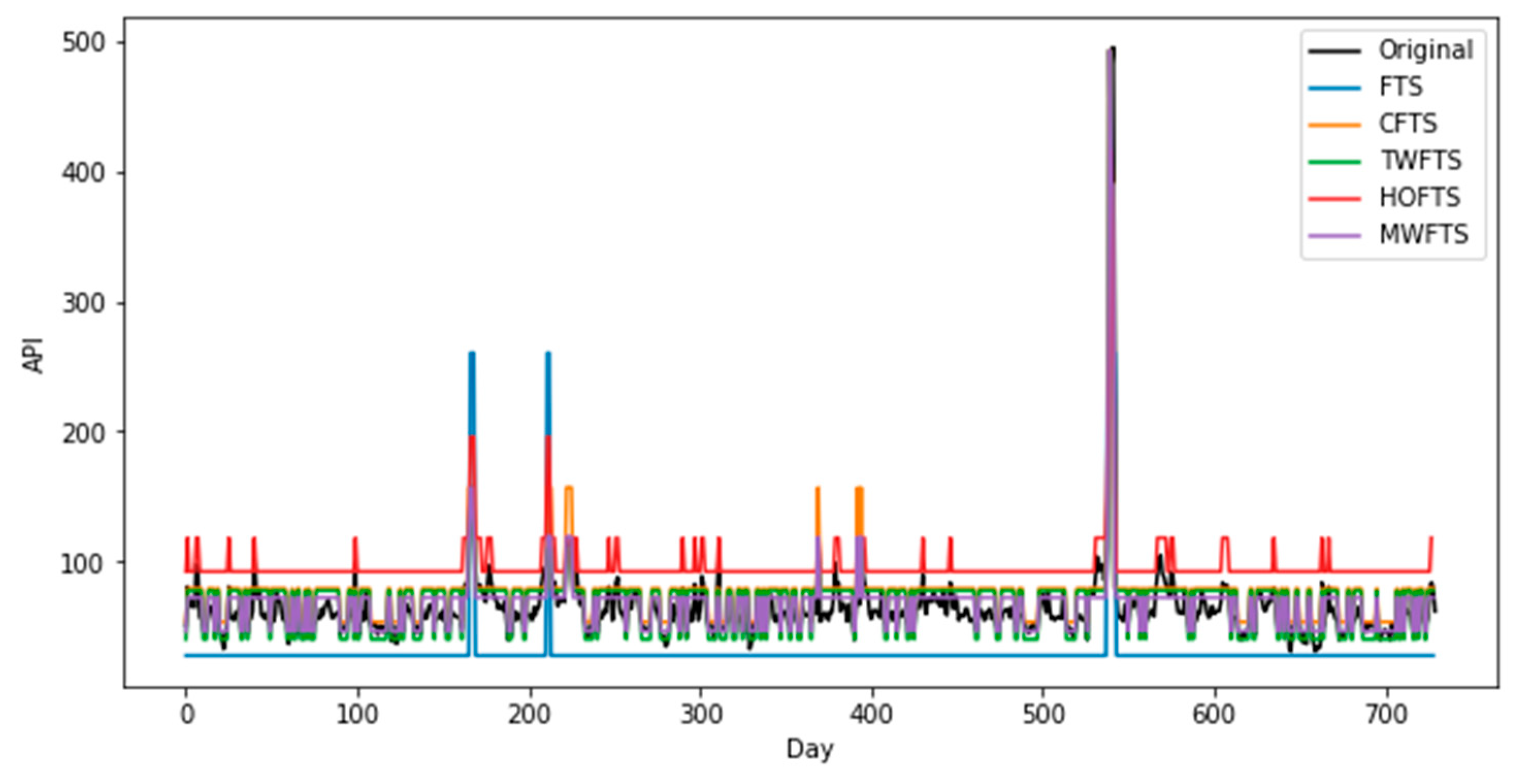
For validating the proposed model, the testing and training dataset of the APIs are used to evaluate the model performance and compare it with some of the famous existing models. Particularly, we introduce a comparison between the FTSMC model based on the optimal number of partitions and conventional FTS models that were proposed by Song & Chissom [18], Chen [21], Cheng [47], and Severiano et al. [48], which are FTS [18], CFTS [21], TWFTS [47], and HOFTS [48], respectively, to examine the performance of the proposed model. It can be seen from Table 7 and Figure 8 that the performance of the proposed model using the training dataset is very good. It has been performed with the smallest values of RMSE, MAPE, and U statistic as compared to other forecasting models. Thus, the proposed model outperformed the other forecasting models. This indicates that the proposed model is a powerful model for predicting air pollution occurrences. In addition, it could be seen from Table 8 and Figure 9 that the proposed model, using the testing dataset, outperformed the other FTS models. This implies that the model can produce a better forecasting accuracy of air pollution, which indicates that the proposed model can be modeled very well using any sort of time series.
In addition, a comparison of the proposed model and some of the famous existing time series models are presented for further validation of our model. The time series models are ARMA [1], ARIMA [5,49], exponential smoothing [49], SARIMA [50], autoregressive conditional heteroskedasticity (ARCH) [51], GARCH [51], Markov chain [3], and fuzzy-ARIMA [52]. The evaluation of the model has been done based on the Akaike information criterion (AIC) [53] and Bayesian information criteria [54] using Equations (11) and (12), respectively, which are the common goodness of fit criteria for selecting the best time series models.
A I C = 2 k r   ln ( L )
B I C = k   ln ( r ) r   ln ( L )
where r is the number of observations, and k is the number of parameters used in models, and L = L ( θ ^ )   is the maximum value of the likelihood function of the model, which can stand for mean square error ( M S E ) . It could be seen from Table 9 that the proposed model produced the smallest values of AIC and BIC compare to the other models. This indicates that the proposed model outperformed the other models; thus, it is an adequate model, and it could provide an accurate forecast of air pollution.
Furthermore, air pollution forecasting is based on daily API concentrations [3,39,45]. According to the time series lag test, as shown in Figure 10, we can effectively develop the performance of the fuzzy time-series Markov chain forecasting model. Based on different testing periods, the time lags of the API time series are not the same.

6. Conclusions

This study proposed the FTSMC model based on the optimal partition number for forecasting the air pollution in Malaysia using daily API data gathered from Klang for a period of three years. In this study, the Markov weights of the fuzzy logical relationships (FLRs) in the FLRG have been calculated based on the Markov transition probability. The grid partition method has been used to determine the optimal partition number of U . Then, the evaluation of the proposed model has been performed using a different number of partitions, which is chosen in order to avoid the arbitrary choosing of intervals. This is considered the first study that has ever properly defined the number of partitions in the FTSMC model. Although, the optimal number of partitions could be developing the model performance. In the proposed forecasting method, fitting the optimal number of partitions provided an improvement in the forecasting accuracy. In forecasting the daily API data, it shows that the proposed model has produced a higher prediction accuracy as compared to some FTS models. This indicated that the model could be used for forecasting air pollution data, in addition to various time-series data. For future studies, the proposed model could be performed to provide accurate results of air pollution for the sub-index variables such as PM2.5, PM10, O3, SO2, NO2, and CO, including the weather factors, such as wind speed and temperature, to provide a comprehensive exanimation of the air pollution problem. In addition, the proposed model can be developed by utilizing optimization methods such as Kalman filter, topology method, and Bayesian method, which are recommended to be employed in future works to provide an accurate forecasting model to predict air pollution. Additionally, it can be developed by combining the model with clustering and machine learning techniques in order to improve the model forecasting accuracy.
Author Contributions

Project administration, Y.A.; supervision, M.O., R.S., and I.F.; coding Y.A. and P.C.L.S. All authors have read and agreed to the published version of the manuscript.

Funding

This research was funded by the Grant Fundamental Research Grant Scheme (FRGS), Universiti Teknologi PETRONAS, cost center: 015MA0-021.

Acknowledgments

The authors are grateful to University Teknologi PETRONAS for providing financial support and good facilities. Additionally, they are thankful to the Department of Environment Malaysia for providing the air pollution data.

Conflicts of Interest

The authors declare no conflict of interest.

Appendix A

Table A1. List of symbols and abbreviations in the study.
Symbol/AbbreviationDescription
A i Fuzzy set
U Universe of discourse
D m i n The minimum value in the universe of discourse U
D m a x The maximum value in the universe of discourse U
D 1 Positive value
D 2 Positive value
f A i Membership function of fuzzy set
u i Linguistic intervals
F ( t ) Fuzzy time series at time t
FLRFuzzy logical relationships
FLRGsFuzzy logical relationship groups
m k Midpoints of the linguistic intervals u i
P i j Transition probability
N i j Number of transitions
N i . Total number of transitions
P Transition probability matrix
Y ( t ) Actual value
diff ( Y ( t ) ) The difference in actual values
FTSFuzzy time series
FTSMCFuzzy time series Markov chain
ARIMAAutoregressive integrated moving average
ANNArtificial neuron network
SO2Sulphur dioxide
O3Ozone
PM10Particulate matter
CO2Carbon monoxide
NO2Nitrogen dioxide
APIAir pollution index
Thiels’ UThiels’ U statistic.
RMSERoot mean square error
MAPEMean absolute percentage error
FTSFuzzy time series model proposed by Song
CFTSFuzzy time series model proposed by Chen
HOFTSHigh order fuzzy time series model proposed by Severiano et al.
TWFTSTrend weighted fuzzy time series model proposed by Cheng
A I C Akaike information criteria
B I C Bayesian information criteria
SARIMASeasonal autoregressive integrated moving average
ARMAAutoregressive moving average
GARCHGeneral autoregressive conditional heteroskedasticity
ARCHAutoregressive conditional heteroskedasticity
M S E Mean square error
L The maximum value of the likelihood function
ACFAutocorrelation function
PACFPartial autocorrelation function
Table A2. Statistical criteria for fitting the best partition number of the FTSMC model using the training dataset.
PartitionsRMSEMAPETheils U
531.4140.691.63
626.3832.101.37
723.5527.381.22
817.3820.410.90
919.9720.201.04
1017.0820.800.89
1116.1019.810.84
1218.9319.370.98
1313.8517.440.72
1417.3516.770.90
1513.2515.800.69
1614.5415.710.76
1714.4314.970.75
1814.2414.540.74
1913.9514.420.72
2013.8314.190.72
2112.7914.130.66
2212.6814.040.66
2312.5514.020.65
2412.2613.910.64
2512.4114.320.64
2612.6514.460.66
2714.0314.430.73
2813.6314.130.71
2912.1313.690.63
3011.4413.150.59
3112.2513.400.64
3211.9113.060.62
3311.9813.100.62
3411.7713.200.61
3512.3013.220.64
3611.9113.330.62
3711.9913.500.62
3811.6813.260.61
3911.6313.210.60
4011.8913.210.62
4111.8013.350.61
4211.7013.370.61
4311.5013.370.60
4411.5013.200.60
4511.8013.210.61
4612.3113.020.61
4711.5113.210.60
4811.5613.140.60
4911.6212.990.60

References

  1. Wang, L.; Wang, J.; Tan, X.; Fang, C. Analysis of NOx Pollution Characteristics in the Atmospheric Environment in Changchun City. Atmosphere 2020, 11, 30. [Google Scholar] [CrossRef] [Green Version]
  2. Kumar, A.; Goyal, P. Forecasting of Daily Air Quality Index in Delhi. Sci. Total Environ. 2001, 409, 5517–5523. [Google Scholar] [CrossRef] [PubMed]
  3. Alyousifi, Y.; Masseran, N.; Ibrahim, K. Modeling the stochastic dependence of air pollution index data. Stoch. Environ. Res. Risk Assess. 2018, 32, 1603–1611. [Google Scholar] [CrossRef]
  4. Rahman, N.H.A.; Lee, M.H.; Suhartono, M.T.L. Evaluation performance of time series approach for forecasting air pollution index in Johor, Malaysia. Sains Malays. 2016, 45, 1625–1633. [Google Scholar]
  5. Box, G.E.P.; Jenkins, G.M. Time Series Analysis: Forecasting and Control, 1st ed.; Holden-Day: San Francesco, CA, USA, 1976. [Google Scholar]
  6. David, G.S.; Rizol, P.M.S.R.; Nascimento, L.F.C. Fuzzy computational models to evaluate the effects of air pollution on children. Rev. Paul. De Pediatr. 2018, 36, 10–16. [Google Scholar] [CrossRef] [PubMed] [Green Version]
  7. Elangasinghe, M.A.; Singhal, N.; Dirks, K.N.; Salmond, J.A. Development of an ANN-based air pollution forecasting system with explicit knowledge through sensitivity analysis. Atmos. Pollut. Res. 2014, 5, 696–708. [Google Scholar] [CrossRef] [Green Version]
  8. Rahman, N.H.A.; Lee, M.H.; Latif, M.T. Artificial neural networks and fuzzy time series forecasting: An application to air quality. Qual. Quant. 2015, 49, 2633–2647. [Google Scholar] [CrossRef]
  9. Bernard, F. Fuzzy environmental Decision-making: Applications to Air Pollution. Atmos. Environ. 2003, 37, 1865–1877. [Google Scholar]
  10. Heo, J.-S.; Kim, D.-S. A New Method of Ozone Forecasting Using Fuzzy Expert and Neural Network Systems. Sci. Total Environ. 2004, 325, 221–237. [Google Scholar] [CrossRef]
  11. Morabito, F.C.; Versaci, M. Fuzzy Neural Identification and Forecasting Techniques to Process Experimental Urban Air Pollution Data. Neural Netw. 2003, 16, 493–506. [Google Scholar] [CrossRef]
  12. Dincer, N.G.; Akkuş, Ö. A new fuzzy time series model based on robust clustering for forecasting of air pollution. Ecol. Inform. 2018, 43, 157–164. [Google Scholar] [CrossRef]
  13. Aripin, A.; Suryono, S.; Bayu, S. Web based prediction of pollutant PM10 concentration using Ruey Chyn Tsaur fuzzy time series model. In Proceedings of the 2016 Conference on Fundamental and Applied Science for Advanced Technology (Confast 2016), Yogyakarta, Indonesia, 25–26 January 2016; pp. 20–46. [Google Scholar]
  14. Hong, W.A.; Man, J.I.; Yili, T.A. Air Quality Index Forecast Based on Fuzzy Time Series Models. J. Residuals Sci. Technol. 2016, 13. [Google Scholar]
  15. Mishra, D.; Goyal, P. Neuro-fuzzy approach to forecast NO2 pollutants addressed to air quality dispersion model over Delhi, India. Aerosol Air Qual. Res. 2016, 16, 166–174. [Google Scholar] [CrossRef] [Green Version]
  16. Darmawan, D.; Irawan, M.I.; Syafei, A.D. Data Driven Analysis using Fuzzy Time Series for Air Quality Management in Surabaya. Sustinere J. Environ. Sustain. 2017, 1, 57–73. [Google Scholar] [CrossRef] [Green Version]
  17. Cheng, C.H.; Huang, S.F.; Teoh, H.J. Predicting daily ozone concentration maxima using fuzzy time series based on a two-stage linguistic partition method. Comput. Math. Appl. 2011, 62, 2016–2028. [Google Scholar] [CrossRef] [Green Version]
  18. Song, Q.; Chissom, B.S. Forecasting enrollments with fuzzy time series-Part I. Fuzzy Sets Syst. 1993, 54, 1–10. [Google Scholar] [CrossRef]
  19. Song, Q.; Chissom, B.S. Forecasting enrollments with fuzzy time series-Part II. Fuzzy Sets Syst. 1994, 54, 1–10. [Google Scholar] [CrossRef]
  20. Zadeh, L.A. Fuzzy sets. Inf. Control. 1965, 8, 338–353. [Google Scholar] [CrossRef] [Green Version]
  21. Chen, S.M. Forecasting enrollments based on fuzzy time series. Fuzzy Sets Syst. 1996, 81, 311–319. [Google Scholar] [CrossRef]
  22. Huarng, K. Effective lengths of intervals to improve forecasting in fuzzy time series. Fuzzy Sets Syst. 2011, 123, 387–394. [Google Scholar] [CrossRef]
  23. Huarng, K.; Yu, T.H.-K. Ratio-based lengths of intervals to improve fuzyy time series forecasting. Ieee Trans. Syst. Man Cybern. Part B Cybern. 2006, 36, 328–340. [Google Scholar] [CrossRef] [PubMed]
  24. Yolcu, U.A. new approach based on optimization of ratio for seasonal fuzzy time series. Iranian J. Fuzzy Syst. 2016, 13, 19–36. [Google Scholar]
  25. Yu, H.-K. Weighted fuzzy time series models for TAIEX forecasting. Physica A: Stat. Mech. Appl. 2005, 349, 609–624. [Google Scholar] [CrossRef]
  26. Cheng, C.H.; Chen, T.L.; Teoh, H.J.; Chiang, C.H. Fuzzy time series based on adaptive expectation model for TAIEX forecasting. Expert Syst. Appl. 2008, 34, 1126–1132. [Google Scholar] [CrossRef]
  27. Efendi, R.; Ismail, Z.; Deris, M.M. Improved weight Fuzzy Time Series as used in the exchange rates forecasting of US Dollar to Ringgit Malaysia. Int. J. Comput. Intell. Appl. 2013, 12, 13–29. [Google Scholar] [CrossRef]
  28. Tsaur, R.C. A fuzzy time series-Markov chain model with an application to forecast the exchange rate between the Taiwan and US dolar. Int. J. Innov. Comput. Inf. Control. 2012, 8, 1349–4198. [Google Scholar]
  29. Sadaei, H.J.; Enayatifar, R.; Abdullah, A.H.; Gani, A. Short-term load forecasting using a hybrid model with a refined exponentially weighted fuzzy time series and an improved harmony search. Inte. J. Elec. P. & Ene. Syst. 2014, 62, 118–129. [Google Scholar]
  30. Egrioglu, E.; Aladag, C.H.; Başaran, M.A.; Uslu, V.R.; Yolcu, U. A new approach based on the optimization of the length of intervals in fuzzy time series. J. Intell. Fuzzy Syst. 2011, 22, 15–19. [Google Scholar] [CrossRef]
  31. Chen, M.Y.; Chen, B.T. A hybrid fuzzy time series model based on granular computing for stock price forecasting. Info.Sci. 2018, 294, 227–241. [Google Scholar] [CrossRef]
  32. Talarposhti, F.M.; Sadaei, H.J.; Enayatifar, R.; Guimarães, F.G.; Mahmud, M.; Eslami, T. Stock market forecasting by using a hybrid model of exponential fuzzy time series. Inter. J. Appro. Reas. 2019, 70, 79–98. [Google Scholar] [CrossRef]
  33. Cheng, C.H.; Yang, J.H. Fuzzy time-series model based on rough set rule induction for forecasting stock price. Neurocomputing 2018, 302, 33–45. [Google Scholar] [CrossRef]
  34. Rahim, N.F.; Othman, M.; Sokkalingam, R.; Abdul Kadir, E. Type 2 Fuzzy Inference-Based Time Series Model. Symmetry 2019, 11, 1340. [Google Scholar] [CrossRef] [Green Version]
  35. Bose, M.; Mali, K. A novel data partitioning and rule selection technique for modeling high-order fuzzy time series. Applied Soft Computing 2018, 63, 87–96. [Google Scholar] [CrossRef]
  36. Zuo, K.T.; Chen, L.P.; Zhang, Y.Q.; Yang, J. Manufacturing-and machining-based topology optimization. Inter. J. adv. Manu. Tech. 2006, 27, 531–536. [Google Scholar] [CrossRef]
  37. Ning, J.; Nguyen, V.; Huang, Y.; Hartwig, K.T.; Liang, S.Y. Inverse determination of Johnson–Cook model constants of ultra-fine-grained titanium based on chip formation model and iterative gradient search. Inter. J. Adv. Manu. Tech. 2018, 99, 1131–1140. [Google Scholar] [CrossRef]
  38. Ning, J.; Liang, S.Y. Inverse identification of Johnson-Cook material constants based on modified chip formation model and iterative gradient search using temperature and force measurements. Inter. J. Adv. Manu. Tech. 2019, 102, 2865–2876. [Google Scholar] [CrossRef]
  39. Koo, J.W.; Wong, S.W.; Selvachandran, G.; Long, H.V. Prediction of Air Pollution Index in Kuala Lumpur using fuzzy time series and statistical models. Air Quality, Atmosphere & Health. 2020, 75, 107–111. [Google Scholar]
  40. Wang, J.; Li, H.; Lu, H. Application of a novel early warning system based on fuzzy time series in urban air quality forecasting in China. Applied Soft Computing. 2018, 71, 783–799. [Google Scholar] [CrossRef]
  41. Yang, H.; Zhu, Z.; Li, C.; Li, R. A novel combined forecasting system for air pollutants concentration based on fuzzy theory and optimization of aggregation weight. Applied Soft Computing 2019, 87, 105972. [Google Scholar] [CrossRef]
  42. DOE Air Quality. Available online: https://www.doe.gov.my/portalv1/en/info-umum/kuality-udara/114 (accessed on 10 April 2019).
  43. DOE Air Pollution Index of Malaysia. Available online: http://apims.doe.gov.my (accessed on 7 January 2020).
  44. DOE Air Quality Standards. Available online: https://www.doe.gov.my/portalv1/en/info-umum/english-airquality-trend/108 (accessed on 31 January 2020).
  45. Alyousifi, Y.; Ibrahim, K.; Kang, W.; Zin, W.Z.W. Markov chain modeling for air pollution index based on maximum a posteriori method. Air Quality, Atmosphere & Health 2019, 1–11. [Google Scholar]
  46. Silva, P.C.d.L.; Lucas, P.O.; Sadaei, H.J.; Guimarães, F.G. pyFTS: Fuzzy Time Series for Python. 2018. [Google Scholar] [CrossRef]
  47. Cheng, C.H.; Chen, T.L.; Chiang, C.H. Trend-Weighted Fuzzy Time-Series Model for TAIEX Forecasting Neural Information Processing. In International Conference on Neural Information Processing; Springer: Berlin/Heidelberg, Germany, 2006; Volume 42, pp. 469–477. [Google Scholar]
  48. Severiano, C.A.; Silva, P.C.; Sadaei, H.J.; Guimarães, F.G. Very short-term solar forecasting using fuzzy time series. In Proceedings of the 2017 IEEE international conference on fuzzy systems (FUZZ-IEEE), Naples, Italy, 9–12 July 2017; pp. 1–6. [Google Scholar]
  49. Syafei, A.D. Applying exponential state space smoothing model to short term prediction of NO2. Jurnal Teknologi. 2015, 9–75. [Google Scholar] [CrossRef] [Green Version]
  50. Lee, M.H.; Rahman, N.; Suhartono, S.; Latif, M.T.; Nor, M.; Kamisan, N. Seasonal ARIMA for forecasting air pollution index: A case study. Am. J. Appl. Sci. 2012, 9, 570–578. [Google Scholar]
  51. Pahlavani, M.; Roshan, R. The comparison among ARIMA and hybrid ARIMA-GARCH models in forecasting the exchange rate of Iran. Inter. J. Busi. Dev. Stu. 2015, 7, 31–50. [Google Scholar]
  52. Tseng, F.M.; Tzeng, G.H.; Yu, H.C.; Yuan, B.J. Fuzzy ARIMA model for forecasting the foreign exchange market. Fuzzy Sets Syst. 2001, 118, 9–19. [Google Scholar] [CrossRef]
  53. Akaike, H. A new look at the statistical model identification. Autom Control IEEE Trans. 1974, 19, 716–723. [Google Scholar] [CrossRef]
  54. Konishi, S.; Kitagawa, G. Bayesian information criteria. In Information criteria and statistical modeling; Springer Science & Business Media: Berlin/Heidelberg, Germany, 2008; pp. 211–237. [Google Scholar]
Figure 1. A method of determination for the APIs.
Symmetry 12 00293 g001
Figure 2. The air monitoring station of Klang.
Symmetry 12 00293 g002
Figure 3. Flowchart of the method.
Symmetry 12 00293 g003
Figure 4. Time series plots of the API values of training data (2012–2013) and testing data (2014).
Symmetry 12 00293 g004
Figure 5. Partition the air pollution index data into several lengths of intervals.
Symmetry 12 00293 g005
Figure 6. The FTSMC model using the grid method with different numbers of partitions using a training dataset.
Symmetry 12 00293 g006
Figure 7. The FTSMC model based on the grid method with the best partition number using a training dataset.
Symmetry 12 00293 g007
Figure 8. Comparison of the proposed model using training dataset with some FTS models proposed by Song and Chissom [18], Chen [21], Cheng [47], and Severiano et al. [48].
Symmetry 12 00293 g008
Figure 9. Comparison of the proposed model using the testing dataset with some FTS models proposed by Song and Chissom [18], Chen [21], Cheng [47], and Severiano et al. [48].
Symmetry 12 00293 g009
Figure 10. Training data lag test.
Symmetry 12 00293 g010
Table 1. Classification of the APIs and health consequences by the Department of the environment of Malaysia [42,44].
StateRange of APIsAir Quality StatusHealth Consequences
1[0, 50]GoodLow pollution without any bad effect on health
2(50, 100]ModerateModerate pollution that does not pose any bad effect on health
3(100, 200]UnhealthyWorsens the health condition of high-risk people that have heart and lung complications
4(200, 300]Very UnhealthyAffects public health. Worsens the health condition and low tolerance of physical exercises for people with heart and lung complications
5(300, ) HazardousHazardous to high-risk people and public health
Table 2. Values of FTS.
No FTS   Values   A i
1 A 0   = 1 u 1 + 0 . 5 u 2 + 0 u 3 + 0 u 4 + + 0 u 27 + 0 u 28 + 0 u 29
2 A 1   = 0 . 5 u 1 + 1 u 2 + 0 . 5 u 3 + 0 u 4 + + 0 u 27 + 0 u 28 + 0 u 29
3 A 2   = 0 u 1 + 0 . 5 u 2 + 1 u 3 + 0 . 5 u 4 + + 0 u 27 + 0 u 28 + 0 u 29
.
.
.
29 A 28   = 0 u 1 + 0 u 2 + 0 u 3 + 0 u 4 + 0 . 5 u 3 + 1 u 27 + 0 . 5 u 28 + 0 u 29
30 A 29   = 0 . 5 u 1 + 1 u 2 + 0 . 5 u 3 + 0 u 4 + + 0 u 27 + 0 . 5 u 28 + 1 u 29
Table 3. APIs as the fuzzy numbers.
NDateAPIFuzzy NumberFuzzy Set Relationships
12012/1/151A0-
22012/1/281A2A0 A2
32012/1/365A1A2 A1
42012/1/470A1A1 A1
52012/1/566A1A1 A1
62012/1/665A1A1 A1
72012/1/798A3A1 A3
.....
.....
.....
7322013/12/2950A0A0 A1
7332013/12/3061A1A1 A1
7342013/12/3170A1A1 A1
Table 4. FLRGs for the grid method with 30 number of partitions.
GroupFuzzy Logical Relationships (FLRs)
G1A0   (4) A0, (4) A1, (1) A3
G2A1   (3) A0, (125) A1, (65) A2, (10) A3, (1) A4
G3A2 (2) A0, (70) A1, (248) A2, (36) A3, (3) A4, (4) A5
G4A3 A1, A2, A3, A4, A5
G5A4 (2) A1, (2) A2, (11) A3, (10) A4, (1) A6, (1) A7
G6A5 (2) A2, (2) A3, (3) A4, A5, A8
G7A6 (1) A4, (1) A5, (1) A6
G8A7   (1) A12
G9A8 (2) A6, (2) A8
G10A12 (1) A14
G11A14 (1) A3
G12A26 (1) A27
G13A27 (1) A14
Table 5. Markov weighted FTS based on the grid method using 30 number of partitions.
Markov Weights Elements for Each Group
A0 A0(4/9), A1(4/9), A3(1/9)
A1 A0(1/68), A1(125/204), A2(65/204), A3(5/102), A4(1/204)
A2 A0(2/363), A1(70/363), 2(248/363), A3(12/121), A4(1/121), A5(4/363)
A3 A1(2/107), A2(47/107), 3(47/107), A4(10/107), A5(10/107)
A4 A1(2/27), A2(2/27), A3(11/27), A4(10/27), A6(1/27), (1/27)
A5 A2 (2/9), A3 (2/9), A4 (1/9), A5(1/3), A8 (1/9)
A6 A4 (1/3), A5 (1/3), A6 (1/3)
A7 A12 (1)
A8 A6 (1/2), A8 (1/2)
A12 A14 (1)
A14 A3 (1)
A26 A27 (1)
A27 A14(1)
Table 6. Statistical criteria for fitting the best partition number of the FTSMC model using the training dataset.
N. PartitionsRMSEMAPETheils U
531.4140.691.63
1017.0820.800.89
1513.2515.800.69
2013.8314.190.72
2512.4114.320.64
3011.4413.150.59
3512.3013.220.64
4011.8913.210.62
4511.8013.210.61
Table 7. Statistical criteria of the proposed model and some FTS models using the training data.
ModelRMSEMAPETheils U
FTS [18]27.9419.451.45
CFTS [21]15.0822.850.78
TWFTS [47]12.8414.280.62
HOFTS [48]28.6532.961.31
FTSMC The proposed model11.4413.150.59
Table 8. Statistical criterions of the proposed model and some FTS models using the testing data.
ModelRMSEMAPETheils U
FTS [18]46.8061.242.07
CFTS [21]24.2736.631.26
TWFTS [47]18.0618.880.89
HOFTS [48]28.6542.961.49
FTSMC The proposed model17.0117.320.80
Table 9. AIC and BIC criteria of the proposed model and some of the existing models.
Prediction ModelAICBICRanking
ARMA 9389.569425.396
ARIMA9380.539415.824
Markov chain9381.239418.713
ARCH12,213.4712,249.337
GARCH12,225.4212,261.058
SARIMA9385.919421.285
Fuzzy-ARIMA9379.949313.982
Exponential smoothing12,942.5812,977.249
FTSMC The proposed model9368.149406.461