Application of a New Combination Algorithm in ELF-EM Processing

Abstract

With regards to the electromagnetic measurement while drilling (EM-MWD), the extremely-low frequency electromagnetic wave signal (ELF-EM) below 20 Hz is usually used as the carrier of downhole measurement data due to the transmission characteristics of the electromagnetic wave (EM). However, influenced by the low frequency noise of drilling, the ELF-EM signal will be inevitably interfered by field noise, which ultimately impedes decoding. The Fourier band-pass filter can effectively remove out-of-band noise but is incapable of handling in-band noise. Therefore, based on the traditional method, a hybrid algorithm of adaptive Wiener algorithm and correlation detection (AWCD) is designed, so as to enhance the in-band noise processing capability, and the effectiveness of such algorithm is well verified through coding and decoding simulation as well as experimental data. The proposed algorithm, as indicated by theoretical analysis and test data, can effectively solve actual engineering issues, providing methodological references to engineers and technicians.

1. Introduction

Currently, two transmission modes are mostly applied to the measurement while drilling (MWD) process, namely stand pipe for mud pulse detection [1] and electromagnetic (EM) wave transmission [2,3]. As the latter is not dependent on drilling fluid, does not require the balanced pressure between downhole fluid and formation, and can send measured data in real-time, it is becoming the focus of MWD studies along with the development of such new technologies as under-balanced well and air drilling. Despite that, the signal processing capability of the system’s surface receiver has posed a restriction upon its development. It is proven by theoretical studies that the signal strength will gradually decrease as the frequency of the MWD EM wave increases [3]; after taking engineering factors into consideration, ELF-EM below 20 Hz is commonly adopted as the carrier. As exploration deepens, the received EM signal of constant frequency is gradually weakened, interfered with by various noise from field operations and, therefore, affecting decoding accuracy. Effectively improving the processing capacity of the terminal receiver’s algorithm can practically enlarge transmission depth, improve the signal to noise ratio (SNR), and reduce the error rate. Traditionally, designed filtering bandwidth is applied to smooth out-of-band noise [4], which is reliable and sound, and works well for the out-of-band noise, not the in-band noise. In addition, the Fourier transform-based denoising method is suitable for stationary signals, but it has a poor processing effect on non-stationary ELF-EM signals whose frequency changes with time. The key to extend transmission depth and lower decoding error rate is whether the in-band noise of ELF-EM signal can be filtered without affecting signal source. Researchers have proposed different solutions, such as the MWD system signal processing based on wavelet transform and pattern recognition [5] by Dong Xiani, which analyzed MWD channel attenuation features and noise characteristics, and established the signal filtering and recognition model to yield a combined method of wavelet transform, correlation filtering and pattern recognition. However, wavelet parameters need to be set on the basis of pre-analyzing signal features; and for signals with different SNR, the decomposition level of the best denoising effect shall be determined as well, all of which proves unfitting to the non-stationary and mostly real-time ELF-EM signal processing. In the harmonic interference elimination algorithm based on parameter estimation [6] by Long Ling et al., harmonic waves are estimated then reconstructed, with interference signals eliminated from received signals, iterating such processes until effective signals reach more than 50% of the effective signal, whereas this algorithm fails to filter out in-band noises and meet the real-time decoding requirement. Wang Hongliang et al. proposed a correlation adaptor-based EM-MWD signal detection algorithm [7] that carries out EM signal detection according to the initial signal strength and adaptive detection and correlation, but the designed algorithm requires high accuracy and real-time performance of the collected reference noise. The EM-MWD receiver of neural network algorithm proposed by Whitacre et al. [8] has adaptive learning ability, and performs better than correlation receivers, especially for non-white noise and ambient noise obtained from actual drilling sites. ELF-EM signal needs to be decoded in higher real-time efficiency, so the design of its learning algorithm is crucial. The multi-combinational adaptive tracking detection algorithm proposed by Li Fukai et al. [9] designed adaptive notches to obtain the reference noise and then used the adaptive cancellation algorithm to denoise it. This algorithm can eliminate in-band interference to some extent, but it is still difficult to remove in-band noise of large interference. In summary, some of the above methods have their own limits and others perform poorly with regard to in-band noise reduction, all of which is hard to meet the complex conditions of drilling projects. Therefore, to work out an effective method of removing the ELF-EM in-band noise has become a key to the transmission of EM-MWD. Figure 1 shows a typical schematic diagram of EM signal transmission in MWD. In order to study the denoising of ELF-EM signal in MWD, its coding methods and spectral characteristics must be explored first, and then the influencing factors to engineering applications. Furthermore, based on previous studies, this paper designs a combinational algorithm based on the adaptive Winner correlation detection algorithm (or AWCD) to further improve the in-band noise processing ability. By means of codec simulation and actual field data, the effectiveness of such algorithm is verified. Additionally, theoretical analysis and field data processing showed that the algorithm can solve practical engineering problems and provide reference to field technicians.

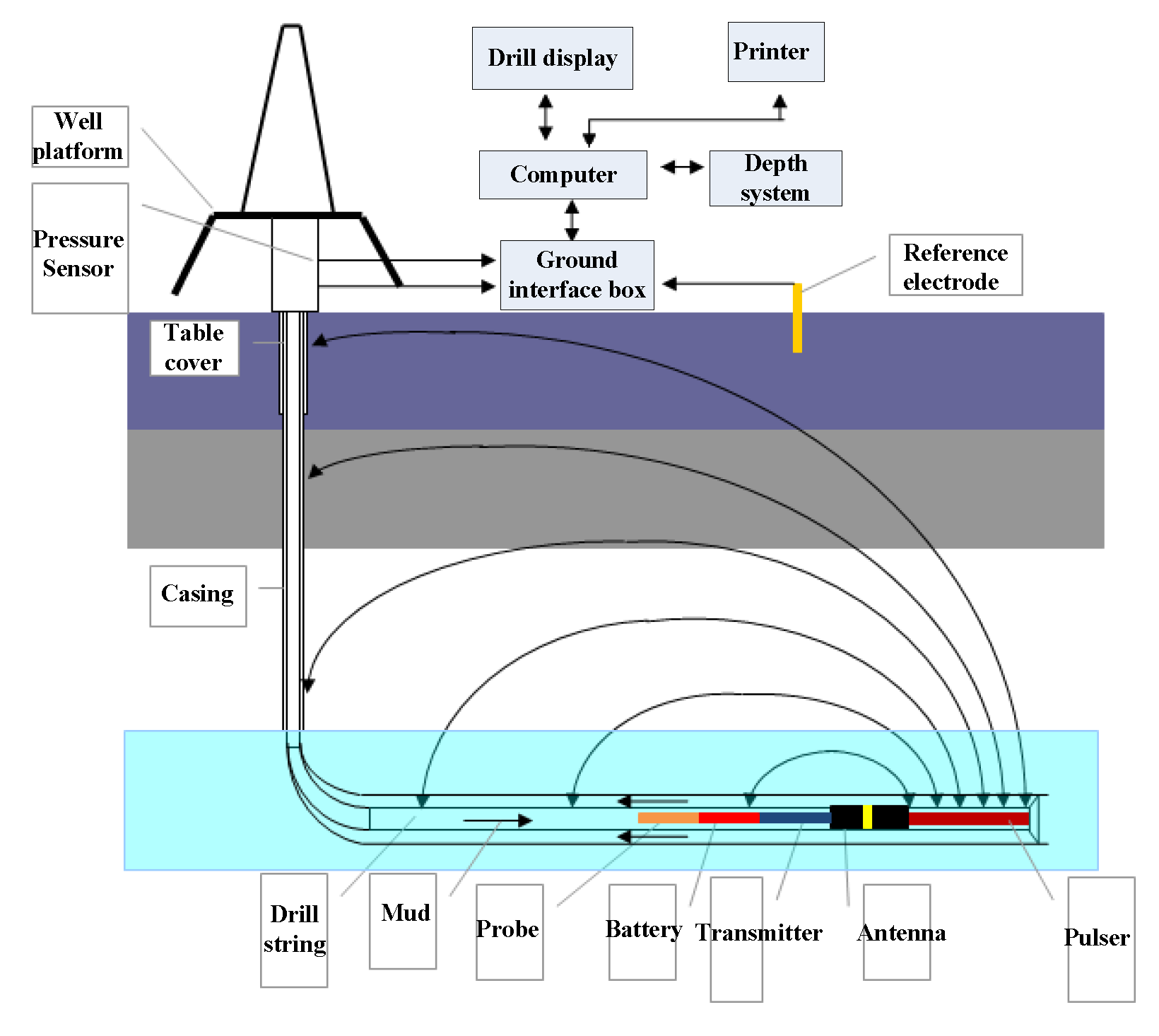
2. The Encoding and Influence Factors of ELF-EM Transmission in Strata

In terms of the transmission characteristics of ELF-EM in strata and the actual needs of MWD projects [10], the frequency of transmitted ELF-EM is usually set below 20 Hz. Pulse position modulation (PPM) uses the relative position of pulses for modulation, of which pulse amplitude and width remain unchanged, thus facilitating modulation and demodulation. In addition, it has higher power utilization rate with relatively low transmission power [11,12,13]. As a result, the EM MWD system is more suitable for PPM modulation. The modulation and demodulation process is shown in Figure 2:

A typical MWD ELF-EM modulated signal is shown in Figure 3 below, and its carrier frequency is 6.25 Hz.

Its data frame formats are:

Frame sync header	Mode word	Data1	Data2	……	Data(2N-1)
S	F	x1	x2	……	xn

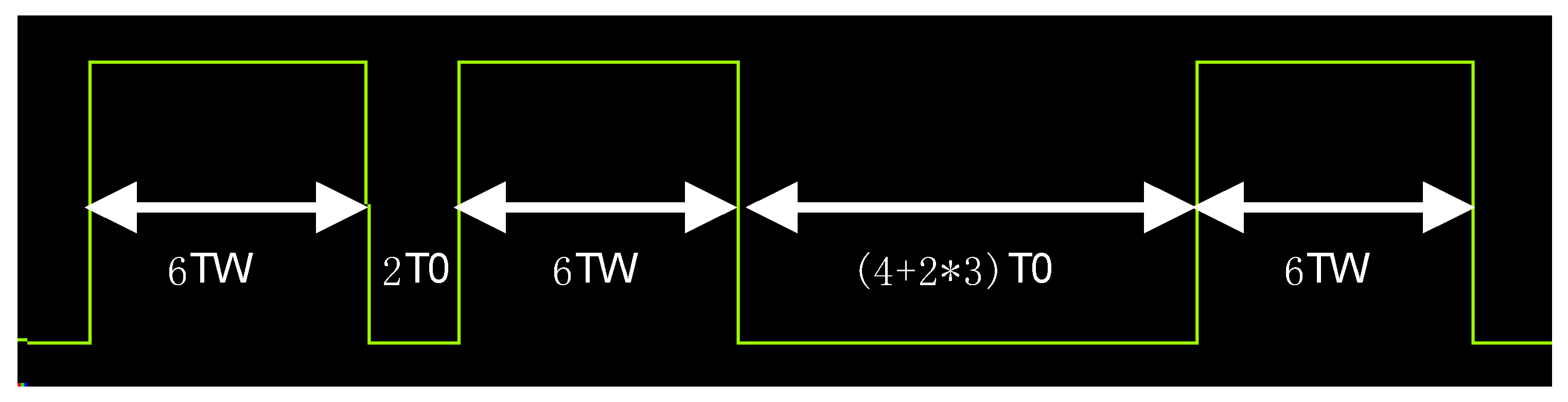
• Data stream: M = 6TW + 2T0 + 6TW + (4 + F × 3) T0 + 6TW + (4 + x1 × 3) T0 + 6 TW + ⋯ + (4 + xn × 3) T0 + 6TW.
• S: S = 6TW + 2T0 + 6TW (TW represents carrier cycle high level, T0 represents carrier cycle low level).
• F: Represents the type of measurement data. F = 0, 1, 2.
• X: Represents the decoding, whose format is X = 6TW + (4 + x × 3) T0 + 6TW, X = x1, x2, …, xn.
• T: The width of a code.
• S2 waveform envelope detection is shown in Figure 4.

The frequency domain analysis of Figure 4 is shown in Figure 5. It can be seen that the modulated signal frequency is distributed in relatively the lower frequency band below 20 Hz. and the main spectrum energy is concentrated in the 4~8 Hz frequency band.

According to the carrier modulation signal, the passband of the band-pass filter can be set to 4~8 Hz. However, this traditional filtering method cannot solve the problem caused by in-band noise interference that will affect or even stem decoding. The influence factors (interference sources) of the ELF-EM transmission process are analyzed here [14]: the ELF-EM signal is unavoidably subject to a large amount of low-frequency and high-frequency noise interference during transmission. Low-frequency noise, ranging from 0 to 10 Hz, is mainly caused by mechanical vibrations, like pump stroke, compound rotation, drilling rig sliding, advancing, triplex drilling pump movement, etc. High-frequency noise, ranging from 10 to 100 Hz, is mainly generated by on-site electric operation, bit cone friction, turbo dynamo rotation, screw rotor rotation and the like [15,16]. Additionally, the amplitude of interference noise varies irregularly, causing frequency spectrum aliasing between the signal and interference noise, which ultimately hinders back-end signal processing and decoding.

From the frequency domain analysis of PPM coded signal and the interference noise frequency analysis, there is a great deal of overlap between the frequency spectrum of interference signal and coded signal; so how to effectively remove the low-frequency interference in band has become an urgent issue to be solved in the current ELF-EM signal processing.

3. Filtering Algorithm Analysis

Traditional low-pass filter based on Fourier algorithm and FIR band-pass filter can effectively filter out-of-band noise but is incapable of handling in-band noise. Therefore, based on such traditional filters, a kind of correlation detection method combining adaptive algorithm with FIR Wiener algorithm is designed to further filter out in-band noise and improve the decoding SNR of the back end.

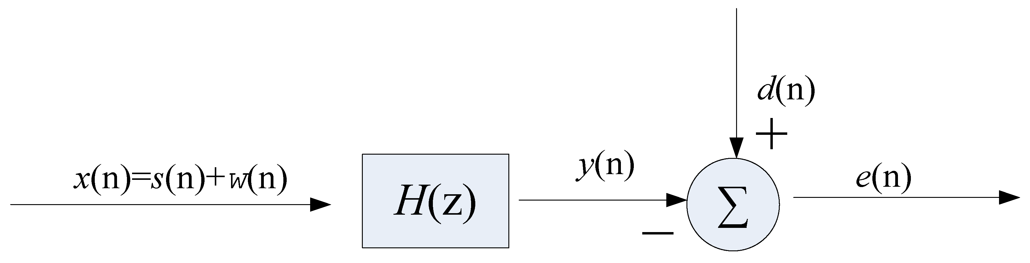
3.1. FIR Wiener Filtering Algorithm

If the received signal is denoted as $x(n)=s(n)+w(n)$, where $s(n)$ is the true signal and $w(n)$ is the noise. Without loss of generality, we can assume $x(n)$, $s(n)$ and $w(n)$ are stationary random signals of zero-mean, or even more simply, real signals. Now is to estimate $s(n)$ from $x(n)$. Let $x(n)$ go through a linear shift invariance (LSI) system $H(z)$ with the output as $y(n)$. The aim of $H(z)$ is to let $y(n)$ approach a certain output $d(n)$, as shown in Figure 6.

Select $d(n)$ as filtering requires [17,18]:

• If $d(n)=s(n)$, then filtering is wrong;
• If $d(n)=s(n+\Delta )$, then pure prediction is wrong;
• If $d(n)=x(n+\Delta )$, then prediction is wrong;
• If $d(n)=s(n-\Delta )$, then signal smoothing is wrong;

In the equation above, $\Delta$ represents a time segment and $\Delta >0$. If $\Delta$ is just a sampling interval, that is, $d(n)=s(n+1)$ or $d(n)=x(n+1)$, then above prediction is also called as one-step prediction. Filtering, prediction and smoothing can be defined as: Filtering is to estimate the data at $t$ in the time segment $0~t$; prediction is to estimate the data at $t_1$ in the time segment $0~t$, where $t_1>t$; and smoothing is opposite to prediction, which is, to estimate the signal at $t_1$ based on the data at time segment $0~t$.

To make $y(n)$ approach $d(n)$ as much as possible, the mean-square error criterion is mostly applied to determine the approach. Define:

$$\epsilon =E\left\{e^2(n)\right\}=E\left\{{\left[d(n)-y(n)\right]}^2\right\}$$

(1)

as the minimum. Since $y(n)=x(n)\ast h(n)$, $\epsilon$ is relative minimum to $h(n)$. Substituting $y(n)$ into Equation (1) yields:

$$\begin{array}{l}\epsilon =E\left\{d^2(n)\right\}-2E\left\{d(n)y(n)\right\}+E\left\{y^2(n)\right\}\\ =E\left\{d^2(n)\right\}-2{\displaystyle \sum _{k=0}^{\infty }h(k)E\left\{d(n)x(n-k)\right\}}\\ +{\displaystyle \sum _{k=0}^{\infty }{\displaystyle \sum _{m=0}^{\infty }h(k)h(m)E\left\{x(n-m)x(n-k)\right\}}}\end{array}$$

(2)

Define:

$$r_d(0)=E\left\{d^2(n)\right\}$$

(3)

$$r_{dx}(k)=E\left\{d(n)x(n-k)\right\}$$

(4)

as the mean square value of $d(n)$, and $d(n)$ is mutually correlated to $x(n)$. Thus, $r_x(k-m)=E\left\{x(n-m)x(n-k)\right\}$ is the self-correlation of signal $x(n)$, thus:

$$\epsilon =r_d(0)-2{\displaystyle \sum _{k=0}^{\infty }h(k)r_{dx}(k)+{\displaystyle \sum _{k=0}^{\infty }{\displaystyle \sum _{m=0}^{\infty }h(k)h(m)r_x(k-m)}}}$$

(5)

which is the target function. Define $\epsilon$ as relative minimum to $h(k)$, which is:

$$\frac{\partial \epsilon }{\partial h(k)}=-2r_{dx}(k)+2{\displaystyle \sum _{m=0}^{\infty }h(m)r_x(k-m), k=0,1,}\cdots ,\infty$$

(6)

and let Equation (6) equal to 0, to yield the best filter coefficient in terms of the minimum mean square error, and marked as $h_{opt}(k)$, which yields:

$${\displaystyle \sum _{m=0}^{\infty }{h}_{opt}(m)r_x(k-m)=r_{dx}(k),} k=0,1,\cdots ,\infty$$

(7)

and the mean square error as well:

$${\epsilon }_{\min }=r_d(0)-{\displaystyle \sum _{k=0}^{\infty }{h}_{opt}(k)r_{dx}(k)}$$

(8)

Equation (7) is the Wiener—Hoof Equation and the best filtering coefficient $h_{opt}(n)$, $n=0,1,\cdots ,\infty$ is called as the Wiener solution.

$h_{opt}(n)$ in Equation (7) is infinite. Assume it is FIR filter, which is $h_{opt}(m)$, $m=0,1,\cdots ,M-1, M<\infty$, and Equation (7) can be transformed into:

$${\displaystyle \sum _{m=0}^{M-1}{h}_{opt}(m)r_x(k-m)=rdx(k), k=0,1,\cdots ,M-1}$$

(9)

Define $R_x$ as the autocorrelation matrix (or Toeplitz Matrix) of $M\times M$, $h_{opt}$ as the filtering coefficient matrix of $M\times 1$, composed of $h_{opt}(0),h_{opt}(1),\cdots ,h_{opt}(M-1)$, and $r_{dx}$ as the cross correlation matrix of $M\times 1$, consisting of $r_{dx}(0),r_{dx}(1),\cdots ,r_{dx}(M-1)$. Thus, Equation (9) can take the form of:

$$R_x{h}_{opt}=r_{dx}$$

(10)

Wiener filter coefficient can be obtained through matrix inversion, viz.:

$$h_{opt}=R_x^{-1}{r}_{dx}$$

(11)

and the minimum mean square error is:

$${\epsilon }_{\min }=r(0)d-r_{dx}^T{R}_x^{-1}{r}_{dx}$$

(12)

3.2. Adaptive Algorithm

Commonly applied adaptive algorithms include LMS, NLMS, RLS, etc. The adaptive linear spectrum enhancement algorithm (ALE) of NLMS is used here to further remove in-band noise. See [19,20] for the ALE description.

LMS is the most widely used algorithm, of which the derivation can be found in [19]. However, the stability, speed, and the excess mean square error of its convergence are controlled by step size $\mu$ which is directly relevant to the power of input signal. Thus, a reasonable solution is dividing $\mu$ by signal power so that the stable convergence can be guaranteed while keeping $\mu$ independent from signal power and accelerating the convergence. Specific NLMS algorithm is as follows [18,21]:

Expression of NLMS:

$$h(n+1)=h(n)+\mu (n)e(n)X(n)$$

(13)

Define the variable step size $\mu (n)$ as:

$$\mu (n)=\frac{\alpha }{M{\widehat{P}}_x(n)}$$

(14)

where ${\widehat{P}}_x(n)$ is the estimated signal power at time n:

$${\widehat{P}}_x(n)=\frac{1}{M}{\displaystyle \sum _{k=0}^{M-1}{x}^2(n-k)}=[x^2(n)-x^2(n-M)+P_x(n-1)]/M$$

(15)

As can be seen, ${\widehat{P}}_x(n)$ is time varying and can be obtained by recursion. To converge NLMS, $\alpha$ in Equation (14) shall be:

$$0<\alpha <2$$

(16)

To prevent $\mu (n)$ from approaching extremely large value when ${\widehat{P}}_x(n)$ is excessively small (e.g., the signal is too weak to be captured in certain time segment), Equation (14) can be modified as:

$$\mu (n)=\frac{\alpha }{M{\widehat{P}}_x(n)+c}$$

(17)

where $c$ is a small constant.

3.3. Correlative Filtering Detection Algorithm

Correlation algorithm works well for the detection of noise-interfered signal as it has noise suppression and processing ability, and can reduce error caused by noise when measuring signal amplitude. Define the two sine signals $x(t)$ and $y(t)$ respectively as [22]:

$$x(t)=A\sin (w_{0}t+\phi )$$

(18)

and:

$$y(t)=B\sin (w_{0}t+\phi )$$

(19)

of which the cross-correlation function is:

$$\begin{array}{ll}{R}_{xy}(\tau )& =\frac{1}{2\pi }{\displaystyle {\int }_0^{2\pi }x(t-\tau )y(t)dt}\\ & =\frac{1}{2\pi }{\displaystyle {\int }_0^{2\pi }A\sin [w_0(t-\tau )+\varphi ]\cdot B\sin (w_0+\theta )dt}\\ & =\frac{AB}{2}\cos (w_0\tau +\varphi -\theta )\end{array}$$

(20)

Two signals $x(t)$ and $y(t)$ have the same frequency; if the amplitude of one signal is known, the other’s amplitude can be measured. With correlation method and its noise suppression effect, the error incurred by noise when directly measuring signal amplitude can be well avoided.

The calculation formula of digital signal is:

$$R_{xy}(k)=\frac{1}{N}{\displaystyle \sum _{n=0}^{N-1}y(n)x(x-k)}, k=0,1,2,\dots ,M-1$$

(21)

which can be represented by the matrix:

$$\left[\begin{array}{c}{R}_{xy(0)}\\ R_{xy(1)}\\ ⋮\\ R_{xy(M-1)}\end{array}\right]=\frac{1}{N}\left[\begin{array}{cccc}x(0)& x(1)& \cdots & x(N-1)\\ x(-1)& x(0)& \cdots & x(N-2)\\ ⋮& ⋮& & ⋮\\ x(1-m)& x(2-m)& \cdots & x(N-m)\end{array}\right]\left[\begin{array}{c}y(0)\\ y(1)\\ ⋮\\ y(N-1)\end{array}\right]$$

(22)

Correlation function can be worked out by recursive algorithm in which the previous function result would be updated when sampling the next ($N$th) data, so as to acquire new correlation value. The recursive algorithm goes as follows:

$$\begin{array}{l}{R}_{xy}^N=\frac{1}{N+1}{\displaystyle \sum _{n=0}^{N}x(n-k)y(n)}\\ =\frac{1}{N+1}{\displaystyle \sum _{n=0}^{N-1}x(n-k)y(n)}+\frac{1}{N+1}x(N-k)y(N)\\ =\frac{N}{N+1}{R}_{xy}^{N-1}(k)+\frac{1}{N+1}x(N-k)y(N)\end{array}$$

(23)

where the superscript N in $R_{xy}^N(k)$ represents the estimated value of correlative function at time N, while $N-1$ in $R_{xy}^{N-1}(k)$ stands for the previous value of correlative function.

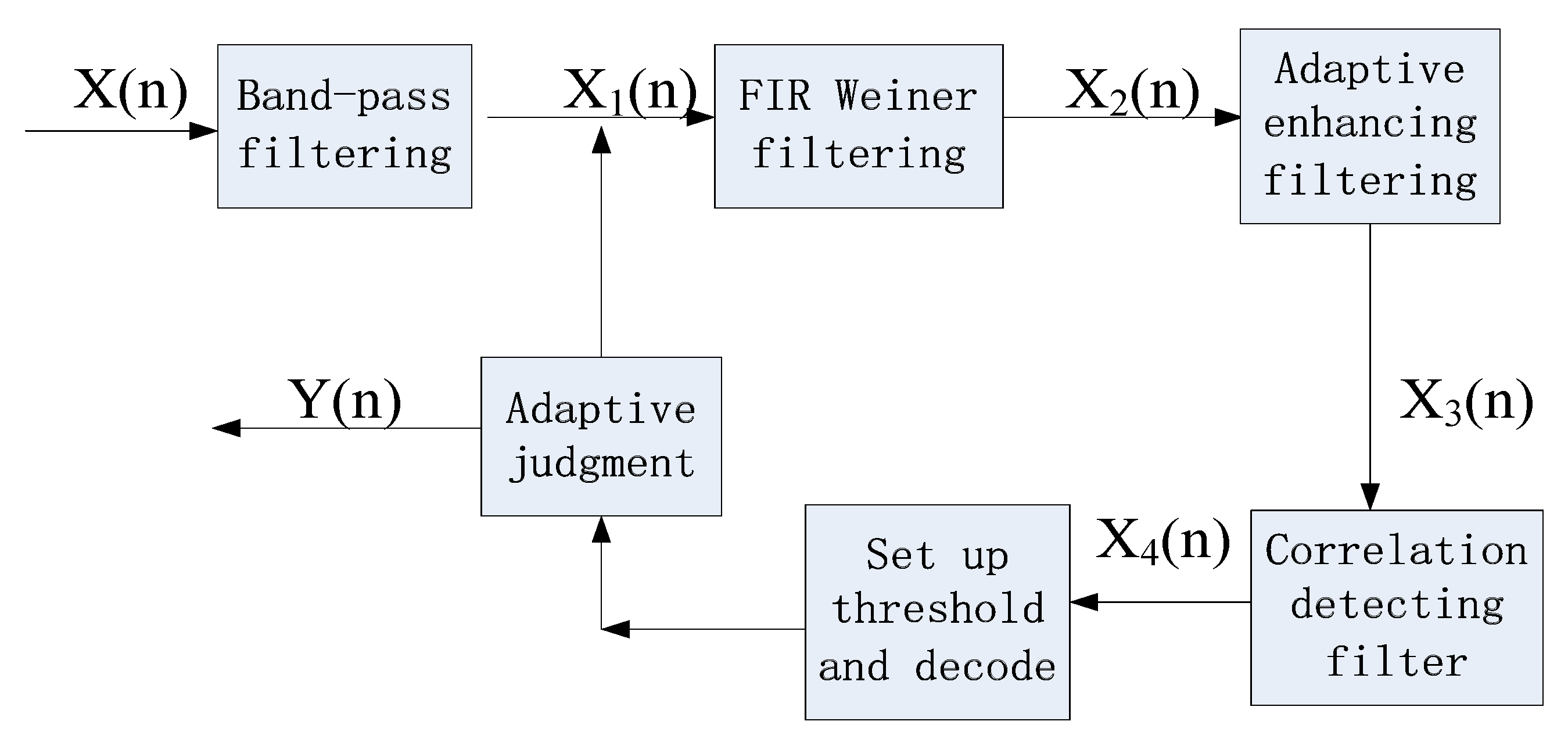
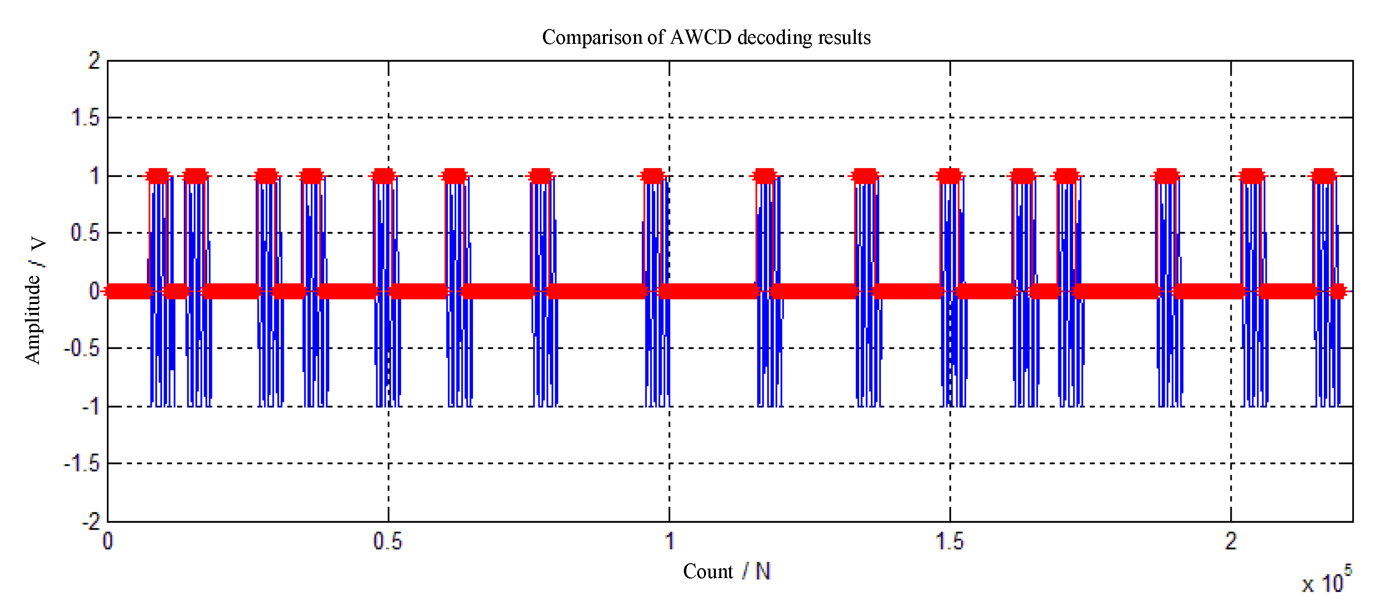
3.4. The Framework of Adaptive Wiener Correlation Detection (AWCD)

Usually, the noise in MWD ELF-EM channel is time changing and unstable, not suitable for statistical analysis and processing. With a certain pass-band, the out-of-band signal can be removed, leaving in-band interference out of handling. To cope with that, based on FIR Wiener filtering and correlation detection, an AWCD algorithm is designed for adaptive denoising. Detailed process is shown in Figure 7 below:

In Figure 7, $\mathrm{X}(n)$ is the surface acquisition signal of interference noise, of which, after band-pass filtering, out-of-band noise can be filtered out of main frequency to yield ${\mathrm{X}}_1(n)$; ${\mathrm{X}}_2(n)$ is the result of ${\mathrm{X}}_1(n)$ after FIR Wiener filtering; and ${\mathrm{X}}_3(n)$ is the detection signal of ${\mathrm{X}}_2(n)$ after adaptive enhancement. With certain detection filtering, the signal ${\mathrm{X}}_4(n)$ is obtained, which is followed by threshold decoding and then goes through adaptive judgment to output $Y(n)$. Such combinational algorithm takes advantages of different algorithms and filters out the ELF-EM out-of-band noise step by step.

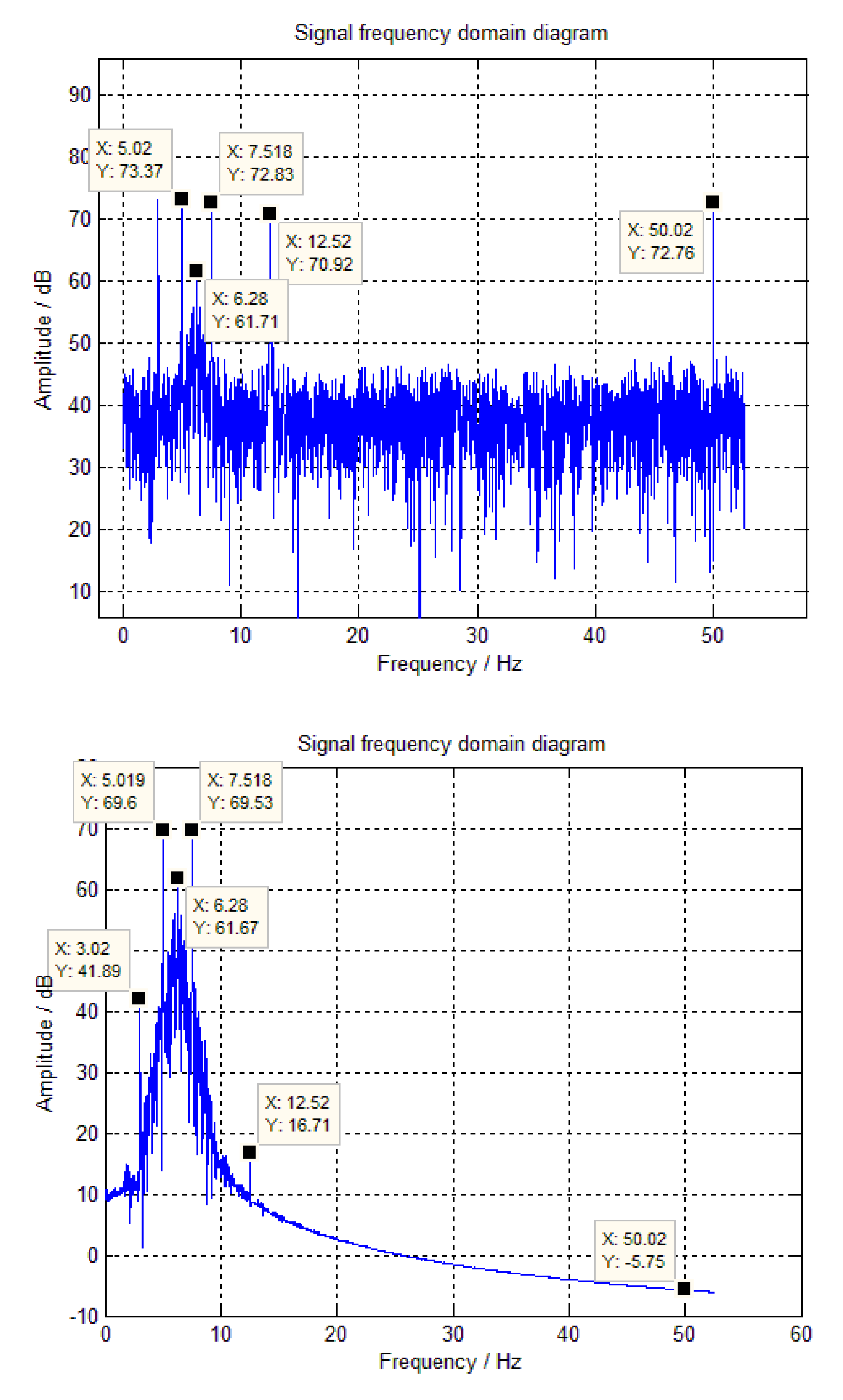
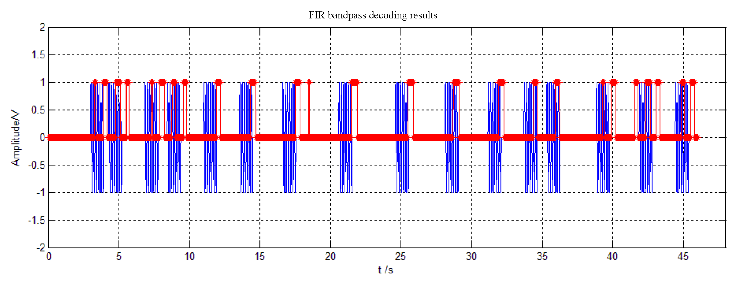
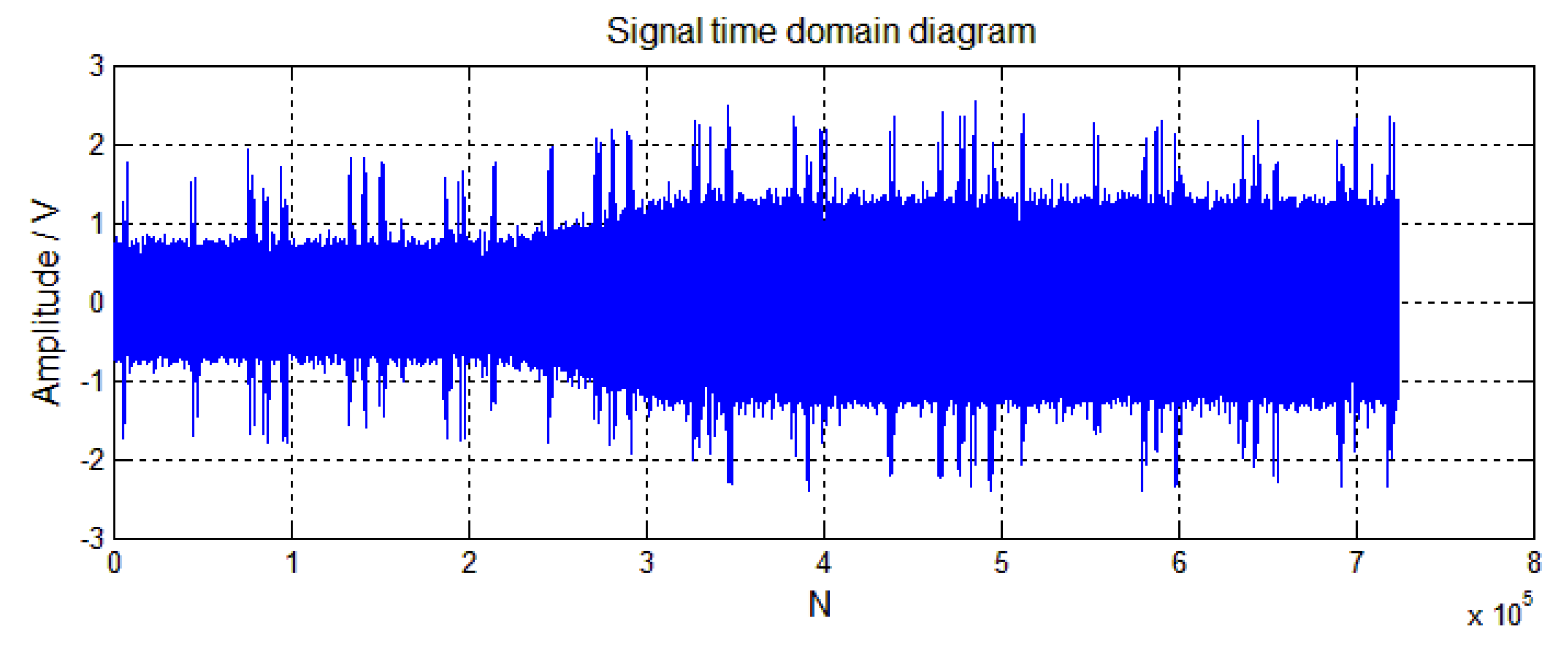
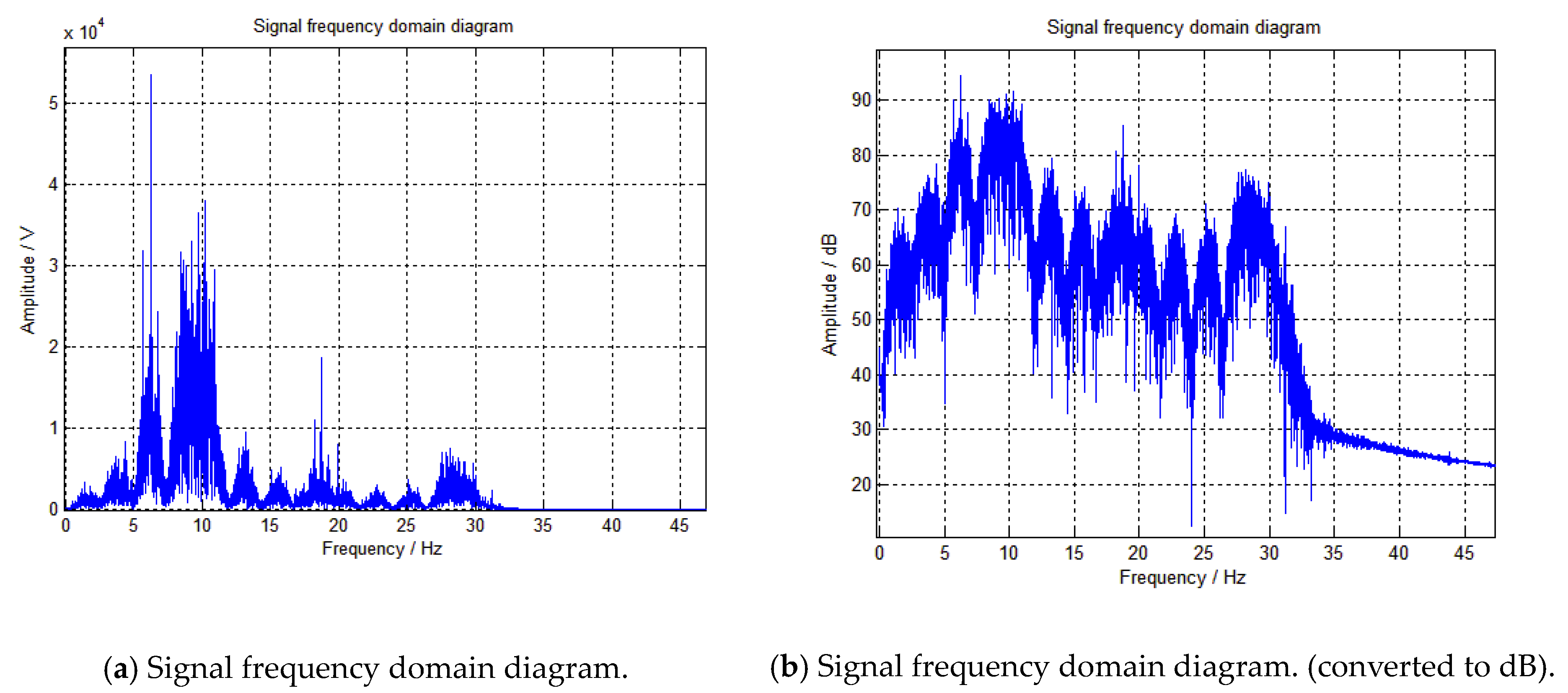
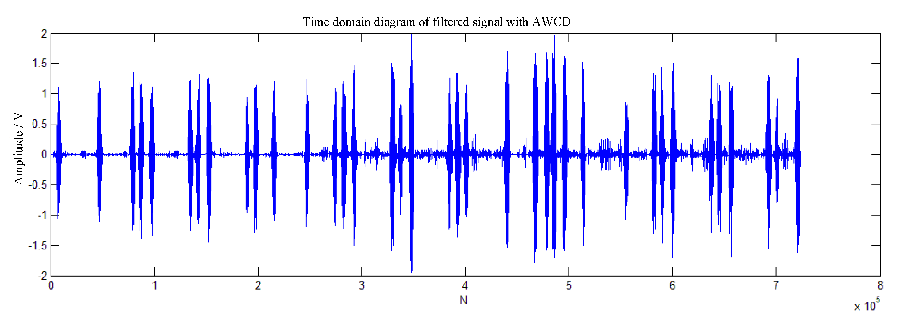
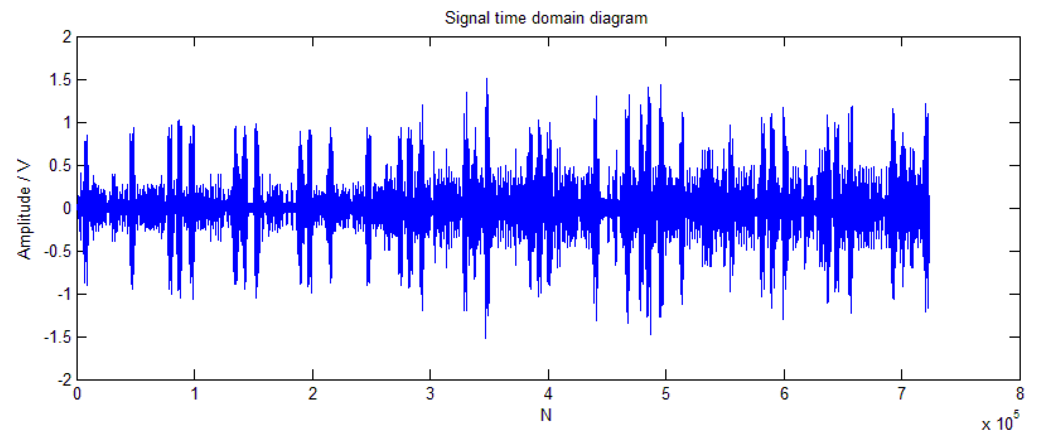
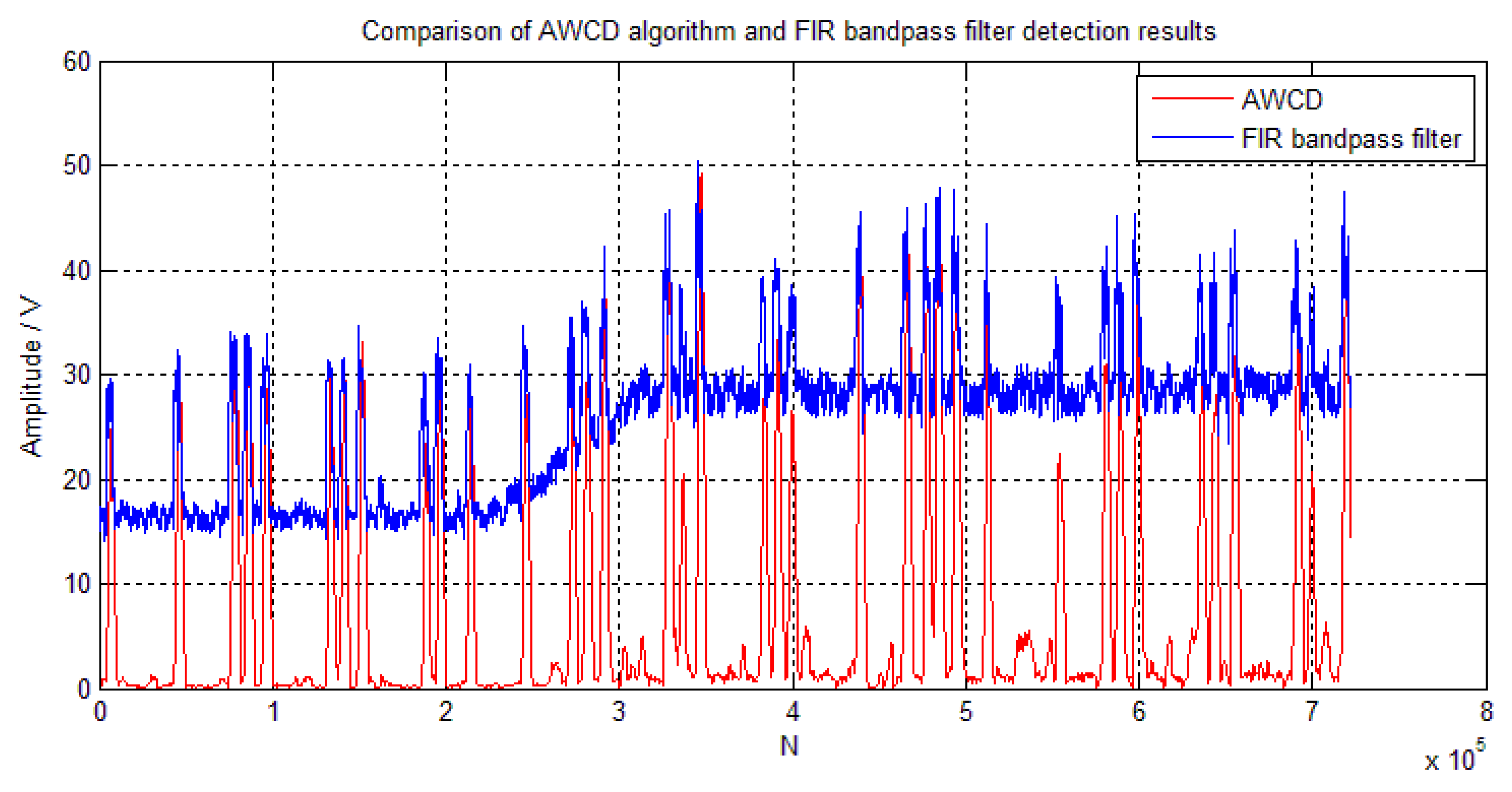
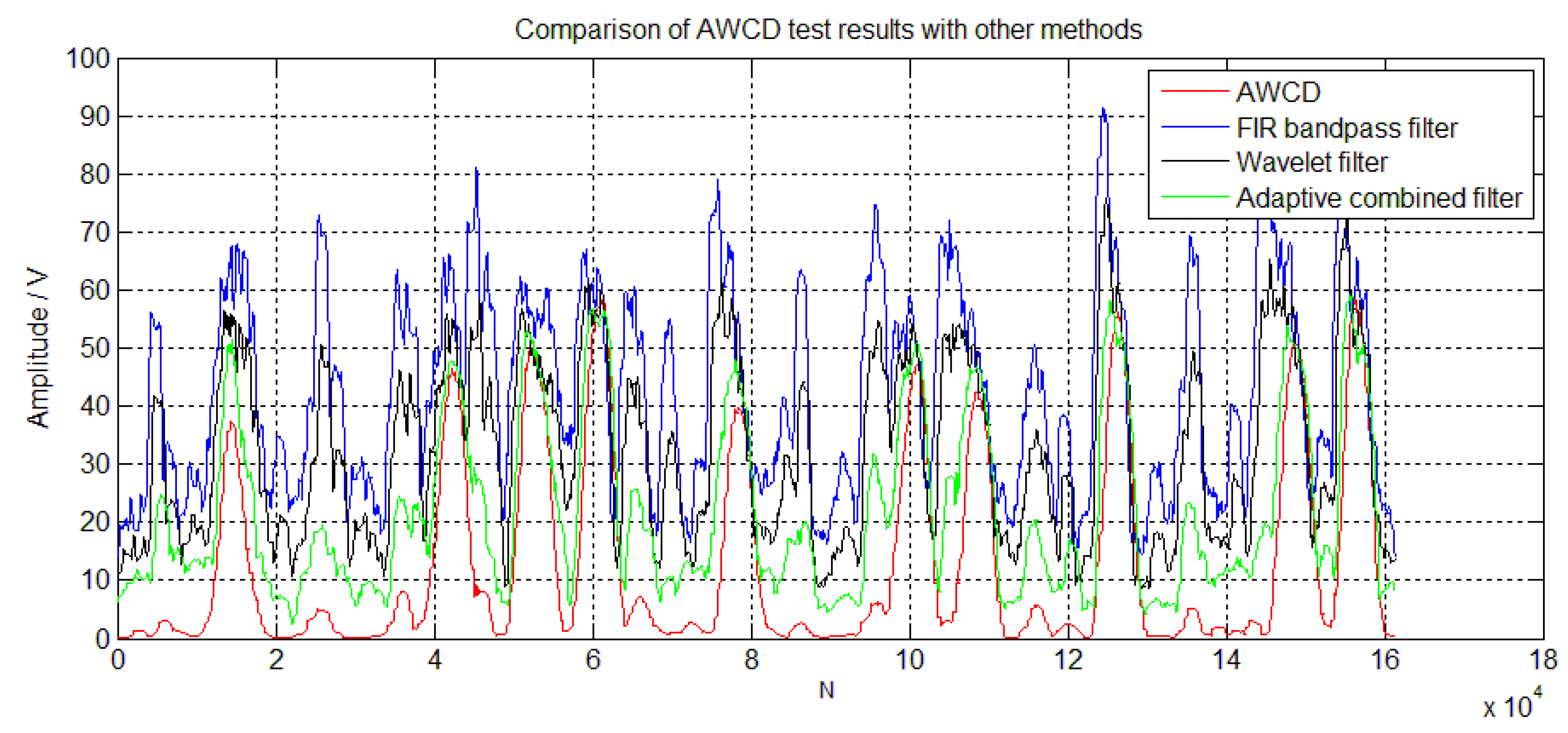
3.5. Simulation Analysis

To testify the operability of AWCD, the MWD signal with various noise is simulated and then processed by AWCD and FIR filtering, respectively. Finally, AWCD detection result will be compared with that of FIR band-pass filtering. Analysis goes as follows:

The comparison between FIR and AWCD results is as follows.

Figure 8 shows the original time domain diagram of EM signal; the coding is S20223554320432 and the carrier main frequency is sine signal of 6.25 Hz.

Figure 9 shows the frequency domain diagram of EM signal before and after FIR band-pass filtering (the filter coefficients are wpl = 5.5, wpu = 7, wsl = 5, and wsu = 7.5, with orders of 128 and sampling rate fs = 200). Interference noise with the same power is added with frequency reaching 3 Hz, 5 Hz, 7.5 Hz, 12.5 Hz, and 50 Hz, together with white noise of equal power. Seen from the result in Figure 9, noise after FIR filtering drops by 31.4 dB, 3.1 dB, 3.3 dB, 54.2 dB, and 79.3 dB respectively.

Figure 10 shows the frequency domain diagrams of ELF-EM signal before and after AWCD filtering. When interference noise frequency reaches 3 Hz, 5 Hz, 7.5 Hz, 12.5 Hz, and 50 Hz, respectively, noise frequency drops correspondingly by 22.3 dB, 20.8 dB, 14.8 dB, 44.9 dB, and 58.5 dB after Wiener filtering (a 6.3 dB increase is seen at 6.25 Hz).

Figure 11 gives the comparison between time domain diagrams of FIR and AWCD filtering effect. It is clearly shown that AWCD has better filtering performance than FIR, which means AWCD can remove the in-band interference signal with larger efficiency and has a lower influence on the original EM signal.

With the above comparison between the data and time domain diagram of FIR band-pass filtering and of AWCD algorithm filtering, a conclusion can be drawn: (1) For interference at around main frequency points (5 Hz and 7.5 Hz), AWCD has obvious advantages over FIR (17.7 dB and 11.5 dB increase); (2) FIR performs better in terms of interference out of main frequency (5 Hz), as compared with data before and after 3 Hz, 12.5 Hz, and 50 Hz filtering; and (3) AWCD is closer to original signal than FIR; FIR filters out interference signal and the out-of-band spectrum of EM original signal at the same time.

Then compare AWCD with FIR band-pass correlation detection; the result is shown in Figure 12. It can be seen that the detection of AWCD is easier to decode than the traditional way.

Then coherent detection is used to decode and compare the results, as shown in Figure 13 and Figure 14. AWCD result shows a more than 95% overlap ratio with EM waveform, and signal data can be well recovered after setting up certain threshold, with adaptive decision decoding being S20223554320432. In contrast, the overlap ratio between FIR and original EM waveforms is lower with error rate more than 50%, which is caused by the interference at main EM frequency points (5 Hz and 7.5 Hz).

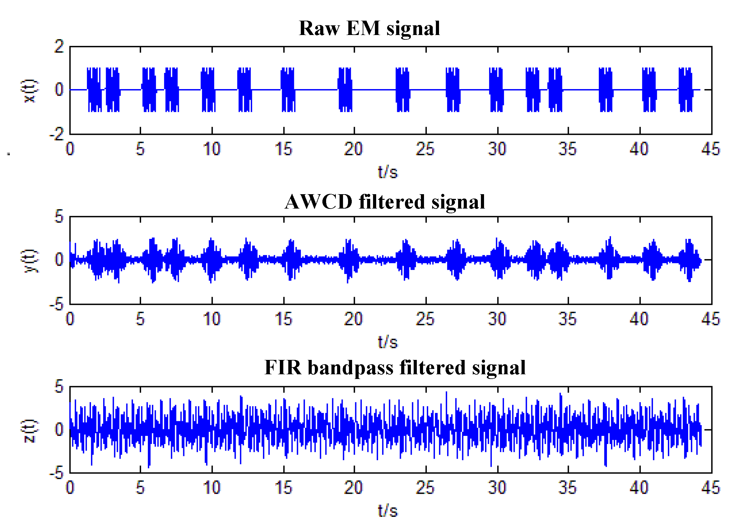
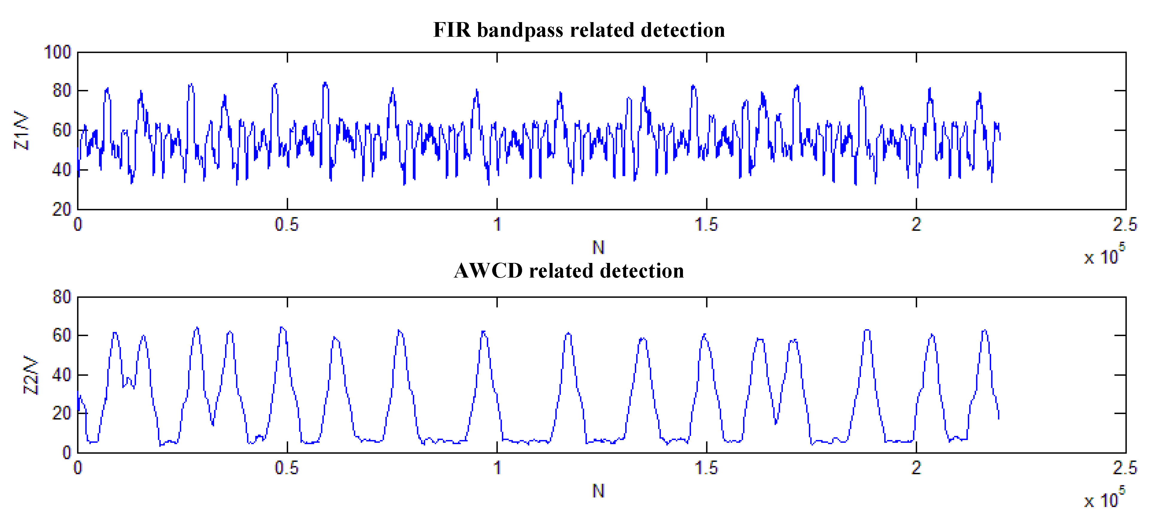
3.6. Analysis and Verification by Field Data

Now, the field EM signal with decoding difficulties (case 1) is used to verify the advantages of AWCD. Figure 15 is the time domain diagram collected on site, from which a strong low-frequency interference can be seen (the high-frequency part has already been filtered out by hardware low-pass). As shown in Figure 16, the interference frequency is within the frequency band of EM signal and overlaps with it, so traditional band-pass filter can exert limited filtering effect.

Figure 17 and Figure 18 are the time and frequency domain diagrams after AWCD processing, and a 35dB increase is seen in SNR. Figure 17 shows a good recovery of time-domain signal out of interfered signal source.

The signal after the FIR band-pass filtering is shown in Figure 19 below, of which the SNR raised by 18 dB as compared with that before filtering. Additionally, in that case, when changed to AWCD, the SNR increased by 18 dB compared with traditional algorithm. Comparing the correlation detection of the two methods in Figure 20, the SNR strength of AWCD is around 17 dB higher than of the FIR. As a result, it has beenproven by field data that the new AWCD algorithm has better anti-interference ability and is easier to decode.

The next case uses the wavelet noise reduction processing algorithm introduced in [5], the band-pass filtering algorithm mentioned in [4], and the multi-combined adaptive tracking detection algorithm mentioned in [9] together with the AWCD combination algorithm proposed in this paper. In Figure 21 are shown the filtering results of each method in separate rows for comparison. From top to bottom are the original signal waveform, using AWCD combination algorithm filtering, FIR band-pass filtering, wavelet noise reduction filtering (the wavelet scale parameter is 7, the wavelet base is a sine wave), and adaptive tracking detection filtering. From the comparison of the filtering results, the AWCD combination algorithm proposed in this paper has the best filtering effect, followed by the adaptive tracking detection algorithm. Figure 22 shows the final detection results of the AWCD combination algorithm and other methods. The AWCD combination algorithm has obvious advantages over the FIR band-pass algorithm, wavelet noise reduction algorithm, and adaptive tracking detection algorithm. This case further validates the engineering practicability of the proposed algorithm.

4. Summary

Due to the complicated MWD engineering situation, the ELF-EM transmission channel are non-linear and non-stationary, and the amplitude of signal and noise are both uncertain. The combination of band-pass filtering, adaptive filtering, Wiener filtering, and correlation detection can maximally filter out in-band noise in any cases, and can be applied to remove noises from received ELF-EM signal of different SNR. The combination is easy to apply, reliable in filtering, and of universality to the ELF-EM processing, which has been proven to be practical in enhancing the SNR of the received signal and reducing the bit error rate of the MWD communication.

In summary, in geologic exploration and engineering, the ELF-EM transmission channel is time changing, added with strong noise. The surface receiver of EM signal will inevitably be influenced by strata and engineering factors, especially by in-band noise that impacts decoding effect and results in a higher error rate and failure of strata detection. The coding schemes and spectrum interference factors of common ELF-EM signal in MWD are analyzed first, with the disadvantages of the traditional algorithm pointed out. AWCD is then proposed to filter out in-band noise and improve decoding SNR. By means of simulation analysis and running with collected in-field data, AWCD is proven to be able to efficiently remove engineering interference noise for decoding, laying the data foundation for drilling and engineering detection.

In the future, work will be done in the following areas to further improve SNR and increase transmission distance: (1) research on signal enhancement from the perspective of array signals or MIMO by adding distributed antennas; (2) study the communication relay problem of drill pipe relay transmission; and (3) multi-channel data fusion analysis (using neural network algorithms [23,24], etc.).

References

1. Reeves, M.; MacPherson, J.; Zaeper, R.; Bert, D.R.; Shursen, J.; Armagost, W.K.; Pixton, D.S.; Hernandez, M. High-speed drillstring telemetry network enables new real-time drilling and measurement technologies[C]HIADC/SPE Drilling Conference. Soc. Pet. Eng. 2006, 1017–1022. Available online: https://www.onepetro.org/conference-paper/SPE-99134-MS (accessed on 13 January 2020).
2. Trofimenkoff, F.N.; Segal, M.; Klassen, A.; Haslett, J.W. Characterization of EM downhole-to-surface communication links. IEEE Trans. Geosci. Remote. Sens. 2000, 38, 2539–2548. [Google Scholar]
3. Fan, Y.H.; Li, W.; Nie, Z.P.; Yang, Z.Q.; Sun, X.Y. Analysis of EM-MWD channel based on NMM. Chin. J. Geophys. 2016, 59, 1125–1130. [Google Scholar]
4. Lu, C.D.; Du, H.B.; Wang, J.H.; Zhang, C. A Design of EM-MWD Signal Receiver Circuit Based on STM32. Chin. J. Eng. Geophys. 2015, 12, 423–427. [Google Scholar]
5. Dong, X.N.; Wang, C.L. MWD system based on wavelet transformation and pattern recognition communication signal processing method and research. Electron. Meas. Technol. 2016, 39, 146–149. [Google Scholar]
6. Long, L.; Chen, Q.; Liu, F. Research on eliminating interference signal algorithm of EM-MWD. Chin. J. Sci. Instrum. 2014, 35, 2144–2152. [Google Scholar]
7. Wang, H.L.; Hong, H.B.; Jiang, G.S.H. Design of EM-MWD signal detection system based on correlation andadaptive filter. Chin. J. Sci. Instrum. 2012, 33, 1013–1018. [Google Scholar]
8. Whitacre, T.; Yu, X.H. A neural network receiver for EM-MWD baseband communication systems. IJCNN IEEE 2009, 3360–3364. Available online: https://ieeexplore.ieee.xilesou.top/abstract/document/5178838 (accessed on 13 January 2020).
9. Li, F.K.; Yang, Z.Q.; Fan, Y.H.; Hao, C.; Zhu, G.; Jin, Y.; Fang, J.; Li, T. Multiple Combinational Algorithm to Adaptively Track and Detect Measurement While Drilling Electromagnetic Wave Signal. IEEE Conf. Publ. (ISAPE) 2018, 1–5. Available online: https://ieeexplore.ieee.xilesou.top/abstract/document/8634120 (accessed on 13 January 2020).
10. Fan, Y.H.; Nie, Z.P.; Li, T.L. EM channel theory model and characteristics analysis for MWD. Chin. J. Radio Sci. 2013, 28, 909–914. [Google Scholar]
11. Li, C. Mathematical Modeling and Signal Characteristics Analysis of Drilling Fluid Pressure MPSK Signal Based on Pulse Width and Pulse Position Modulation. Master Thesis, China University of Petroleum, Qingdao, China, 2010. [Google Scholar]
12. Hamkins, J. Pulse Position Modulation. Handb. Comput. Netw. 2011, 1, 492–508. [Google Scholar]
13. Abdallah, S.A. Turbo Coded Pulse Position Modulation for Optical Communications. Ph.D. Thesis, Georgia Institute of Technology, Atlanta, GA, USA, 2003. [Google Scholar]
14. Macpherson, J.; Gregg, T. Microhole Wireless Steering While Drilling System. Baker Hughes Oilfield Oper. 2007, 19–20. [Google Scholar]
15. Zhao, J.; Wang, L.; Sheng, L.; Wang, J. A nonlinear method for filtering noise and interference of pulse signal in measurement while drilling. Acta Pet. Sin. 2008, 29, 596–600. [Google Scholar]
16. Guo, J.; Liu, H.; Quan, J. Analysis and Control of System Noise in MWD. Oil Field Equip. 2008, 37, 10–13. [Google Scholar]
17. John, G.; Proakis, D.; Manolakis, G. Digital Signal Processing—Principles, Algorithms and Applications, 4th ed.; Publishing House of Electronics Industry: Beijing, China, 2013; pp. 863–871. [Google Scholar]
18. Hu, G.S. Theory, Algorithm and Realization of Digital Signal Process; Tsinghua University Press: Beijing, China, 2012; pp. 246–252, 608–620. [Google Scholar]
19. Li, F.K.; Yang, Z.Q.; Hao, C. Application of weak signal nonlinear detection on MWD electromagnetic Wave. Chin. J. Radio Sci. 2018, 33, 48–55. [Google Scholar]
20. Li, M.Y.; Bai, P. Design of adaptive line enhancement system based on FPGA. Mod. Electron. Technol. 2010, 33, 118–121. [Google Scholar]
21. Zhang, S.; Zhang, J.; Thus, H. Mean square deviation analysis of LMS and NLMS algorithms with white reference inputs. Signal Process. 2017, 131, 20–26. [Google Scholar] [CrossRef] [Green Version]
22. Gao, J.Z. Detection of Weak signals. Available online: https://xs.gufenxueshu.com/books?hl=zhCN&lr=&id=pGSwgjQ9BkgC&oi=fnd&pg=PA5&dq=%E5%BE%AE%E5%BC%B1%E4%BF%A1%E5%8F%B7%E6%A3%80%E6%B5%8B&ots=n4E4hqWrsj&sig=UBbXO1OWJk1d3Zte7HAnd5h8CrY#v=onepage&q=%E5%BE%AE%E5%BC%B1%E4%BF%A1%E5%8F%B7%E6%A3%80%E6%B5%8B&f=false (accessed on 13 January 2020).
23. Li, G.; Wang, J.; Liang, J.; Yue, C.Y. Application of sliding nest window control chart in data stream anomaly detection. Symmetry 2018, 10, 113. [Google Scholar] [CrossRef] [Green Version]
24. Li, G.; Wang, J.; Liang, J.; Yue, C.Y. The application of a double CUSUM algorithm in industrial data stream anomaly detection. Symmetry 2018, 10, 264. [Google Scholar] [CrossRef] [Green Version]
Figure 1. EM MWD system drilling.
Symmetry 12 00337 g001
Figure 2. PPM modulation and demodulation process.
Symmetry 12 00337 g002
Figure 3. Typical MWD ELF-EM modulated signal.
Symmetry 12 00337 g003
Figure 4. S2 waveform envelope.
Symmetry 12 00337 g004
Figure 5. ELF-EM signal frequency domain diagram.
Symmetry 12 00337 g005
Figure 6. Estimation with noise signal.
Symmetry 12 00337 g006
Figure 7. The denoising diagram of AWCD.
Symmetry 12 00337 g007
Figure 8. Simulated EM signal time domain diagram.
Symmetry 12 00337 g008
Figure 9. Comparison between signal frequency domains before and after FIR filtering.
Symmetry 12 00337 g009
Figure 10. Signal frequency domain diagrams before and after Wiener filtering.
Symmetry 12 00337 g010
Figure 11. Filtering effect comparison in time domain diagram.
Symmetry 12 00337 g011
Figure 12. Comparison between AWCD and FIR correlation detection.
Symmetry 12 00337 g012
Figure 13. AWCD decoding diagram.
Symmetry 12 00337 g013
Figure 14. FIR decoding diagram.
Symmetry 12 00337 g014
Figure 15. Time domain diagram of field signal.
Symmetry 12 00337 g015
Figure 16. Frequency domain diagram of field signal.
Symmetry 12 00337 g016
Figure 17. Recovered time domain diagram after AWCD processing.
Symmetry 12 00337 g017
Figure 18. Frequency domain diagram after AWCD processing.
Symmetry 12 00337 g018
Figure 19. Time domain diagram after FIR band-pass processing.
Symmetry 12 00337 g019
Figure 20. Comparison between AWCD and FIR detection.
Symmetry 12 00337 g020
Figure 21. Comparison between AWCD and FIR filtering.
Symmetry 12 00337 g021
Figure 22. Comparison between AWCD and FIR detection.
Symmetry 12 00337 g022