Article

Mathematical Modelling of Ground Truth Image for 3D Microscopic Objects Using Cascade of Convolutional Neural Networks Optimized with Parameters’ Combinations Generators

1
Computer Science, Faculty of Electrical Engineering, University of Sarajevo, 71000 Sarajevo, Bosnia and Herzegovina
2
Université Clermont Auvergne, CNRS, Inserm, GReD, F-63000 Clermont-Ferrand, France
*
Author to whom correspondence should be addressed.
Symmetry 2020, 12(3), 416; https://doi.org/10.3390/sym12030416
Submission received: 13 February 2020 / Revised: 28 February 2020 / Accepted: 2 March 2020 / Published: 5 March 2020

Abstract

:
Mathematical modelling to compute ground truth from 3D images is an area of research that can strongly benefit from machine learning methods. Deep neural networks (DNNs) are state-of-the-art methods design for solving these kinds of difficulties. Convolutional neural networks (CNNs), as one class of DNNs, can overcome special requirements of quantitative analysis especially when image segmentation is needed. This article presents a system that uses a cascade of CNNs with symmetric blocks of layers in chain, dedicated to 3D image segmentation from microscopic images of 3D nuclei. The system is designed through eight experiments that differ in following aspects: number of training slices and 3D samples for training, usage of pre-trained CNNs and number of slices and 3D samples for validation. CNNs parameters are optimized using linear, brute force, and random combinatorics, followed by voter and median operations. Data augmentation techniques such as reflection, translation and rotation are used in order to produce sufficient training set for CNNs. Optimal CNN parameters are reached by defining 11 standard and two proposed metrics. Finally, benchmarking demonstrates that CNNs improve segmentation accuracy, reliability and increased annotation accuracy, confirming the relevance of CNNs to generate high-throughput mathematical ground truth 3D images.

1. Introduction

Deep neural networks (DNNs) along with general concept of deep learning (DL) brought revolution in the area of biomedical engineering, especially medical image processing and segmentation. DL can be described as hierarchical learning that is based on learning characteristics of data. These models are inspired by the flow of information and its processing in the human biological nerve system. CNN networks are a well-known form of DL architecture. When large training datasets are available, DNNs can achieve satisfying results. When real data are not sufficient, it is possible to generate augmented data by data augmentation techniques such as reflection, translation, rotation, etc. Using DNNs for image segmentation in computed topography (CT) [1,2], magnetic resonance (MR) [3,4,5] or X-ray [6,7] images has become standard, while promising results are being obtained with DL in microscopy [8,9,10,11,12,13] and electron microscopy [14,15,16,17,18]. Furthermore, DNNs are successfully implemented for nucleus segmentation [19,20,21,22,23,24,25,26].
One key point in this DL process is the automatic or semi-automatic calculation of mathematical ground truth (mathematical GT) for datasets and several alternatives from various fields have been proposed. Comparison between fine and coarse GT datasets of traffic conditions as well as perspectives of using DNNs to prepare coarse GT datasets are shown in [27]. The CNN called “V-net” associated with data augmentation is successfully used for 3D image segmentation based on a volumetric [28]. V-net achieves better results when compared to solutions presented in the PROMISE 2012 challenge dataset. The CNN network “U–net”, with training strategy that also relies on data augmentation is presented in [29]. U-net outperforms any other solutions at the International Symposium on Biomedical Imaging (ISBI) cell tracking challenge in categories of phase contrast and DIC. Deep Convolutional Neural Network (DCNN) is presented in [30], with focus on having automated training process with usage of tools such as CellProfiler [31] and data augmentation for creation of training dataset. In [32] authors demonstrate multi-class semantic segmentation of CT and MRI images, without specific GT labels, but from different dataset with the same anatomy. Still, it seems that this kind of research is not that common. In addition, majority of state-of-the-art articles tend to optimize single DNN.
Here, machine learning methods and techniques are applied in order to develop robust and objective approach for given problem: generate a GT for Arabidopsis thaliana nucleus dataset. The first part of research [33] uses multiple algorithms, levels and operators to build a model based on traditional unsupervised segmentation methods. After various evaluations, our work shows that the best results on reduced Arabidopsis thaliana dataset are obtained by Generic Ground Truth Image Approach 7 (GGTI AP7) [34]. GGTI AP 7 involves knowledge based optimization and voter and median operators and is implemented with seven unsupervised segmentation algorithms: Adaptive K-means [35,36], Fuzzy-c means [37,38,39], KGB (Kernel Graph Cut) [40,41], Multi Modal [42,43], OTSU [44,45], SRM (Statistical region merging) [46,47] and APC (Affinity Propagation Clustering) [48,49,50].
Although GGTI AP7 gives good results, it also has some flaws. Additional techniques do improve overall results of segmentation, but unsupervised methods can work in unexpected ways in some cases. For example, when using GGTI AP7, some difficulties are encountered for the segmentation of slices at the beginning and at the end of a 3D sample/image stack (where the nucleus is hardly visible or not existing). Furthermore, classical algorithms cannot make semantic segmentation with named output labels, meaning they cannot specifically categorize objects they segment. To overcome these difficulties, this paper focuses on supervised learning techniques, CNNs, semantic segmentation, operators and various optimizations.
This paper offers DL approach with cascade of CNNs (multiple CNNs in sequence) with chained symmetric blocks of layers for semi-automatic mathematical GT generation of Arabidopsis thaliana dataset. It also demonstrates that generated CNNs architecture can be used as pre-trained CNNs and further improvement of generic GT generator. Furthermore, tools and methods developed in this paper can be used for CNN development and generation of mathematical GT for other classes and types of datasets, as illustrated in this paper.

2. Dataset and Methodological Framework

2.1. Dataset Description and Preparation

Images from public OMERO repository at Florida State University, https://omero.bio.fsu.edu/webclient/userdata/?experimenter=-1, (Project: “2015_Poulet et al_Bioinformatics”) are used. The dataset used in this paper is the same as in [51] and is composed of 77 Arabidopsis thaliana nuclei divided in 38 wild type nuclei and 39 nuclei from the crwn1 crwn2 mutant. Microscopic observations are performed using Leica Microsystems MAAF DM 16000B [52]. Samples are saved in TIFF format, and may include a number of 2D multipage slices for each sample. Thus, the dataset provides a full 3D image stack sample collection. The training process of CNN networks requires the same sized input images. As the Arabidopsis thaliana dataset contains samples with variable sizes, appropriate resizing is performed. All samples are less than 110 × 110 pixels, and were resized to 40 × 40 pixels in order to make the training process faster.
The algorithms proposed in this paper process 2D images/slices only. Thus, they cannot be directly applied to 3D stack samples. It is necessary to decompose/compose 3D stack samples into n   x   2 D slices and then compose slices back to 3D stack samples after processing (Figure 1).
As mentioned, GGTI AP7 has drawbacks with segmenting slices at the beginning and at the end of a 3D stack sample, so segmenting and comparing 3D stack samples with all slices would not be useful. Instead, six 3D stack samples are selected—3 from both the wild and mutated classes, with ten slices from middle part of each 3D stack sample. This way it was possible to have reliable and comparable results with GGTI AP7.
In order to generate a training dataset for the CNNs training process and to evaluate proposed algorithms, some sort of GT labelling is necessary. This is done by the manual segmentation of the selected dataset. To make the process of manual segmentation more objective and realistic, 3 team members who are experts in the field, made individual manual segmentations for each slice. To summarize, each expert made 3 manual segmentations for 10 slices of 6 different 3D stack samples (Supplementary Table S1). Individual slices for sample 6 are shown in Figure 2a, and a 3D view of the same sample is shown in Figure 2b.
The subsequent step is to process 3 manual segmentations of every slice through the voter and median operator (voter and median operator will be explained in Section 2.2.1). That is a total of 60 voter and 60 median slice segments for each expert. Corresponding voter and median slices are then processed by the experts through global voter and median operator, resulting in voter and median segments for every slice/3D stack sample. The final voter and median segments of the nucleus are called MGTI (Manual Ground Truth Image). In this study, only voter segments are used for further processing and evaluation. MGTI voter slices for sample 6 are shown in Figure 3a, and a 3D view of same sample is shown in Figure 3b.

2.2. Convolutional Neural Netwotrks (CNNs)

CNN networks are trained with large amounts of data, and can be used in different fields for different purposes such as classification or semantic segmentation. They contain a large number of layers, most of which are convolutional layers. Our proposed CNN architecture uses 2 chained symmetrical blocks of convolutional–batch normalization–ReLu (Rectifier Linear Unit) layers, having max pooling layer between them. The basic architecture of CNN generated in this paper is shown in Figure 4, although GUI tools allow for the additional defining of CNN architecture, such as adding additional convolutional–batch normalization–ReLu blocks of layers in chain.
The input layer is the first layer in the CNN network and it primarily determines input size for the dataset. The input layer size is defined through GUI, and it changes depending on the dataset. Both 40 × 40 pixels and 200 × 200 pixels images are used as will be noted along experiments. Convolutional layer performs convolution operation over layer’s input as defined by filter size. This operation reduces input size, thus enabling faster computing throughout the whole algorithm. Besides reducing input size, convolutional layer produces multiple number of filters as output.
For the first two convolutional layers and transposed convolutional layer, the filter number had double value of previous convolutional layer. Batch normalization layer optimizes input values for further calculations while making no input size changes. ReLu layer applies rectifier linear function to its input while also making no input size changes. Batch normalization layer and ReLu layer have no explicit parameters. Max pooling layer reduces layer’s input size by applying moving window filter size over the whole input, forwarding only the maximum value from that window. The filter size that is used in maximum pooling layer is 2 × 2 pixels, with stride of 2 × 2 pixels. In order to make transposed convolutional layer functional, it is necessary to have input size for the layer calculated correctly. That is why the two convolutional layers preceding the transposed layer must have proper output dimensions. To achieve that, padding must be applied to the input matrices of convolutional layers. The formula for the padding of convolutional layers is:
Padding = { filter   size 2 x filter   size 2   pixels   ,   filter   size = 2 k + 1 ,   k     Z filter   size 2   x   ( filter   size 2 1 ) pixels ,     filter   size = 2 k ,   k ,   k     Z  
Some of previously described layers reduce the size of filters. The transposed convolutional layer applies a transposed convolution operation on filters, computing filters with initial size as output. This layer has filter size of 4 × 4 pixels and stride of 2 × 2 pixels. The cropping of 1 × 1 pixel is due to previously added paddings. Fully connected layer serves as connection between every pixel and previously calculated filters. This convolutional layer has default configuration stride of 1 × 1 pixel, and output of two filters, as there are two labels, background and foreground (nucleus). Softmax layer calculates probability of each pixel belonging to one of two defined labels. Pixel classification layer produces final semantic segmentation, having pixel-labelled output of the same size as the initial input. Softmax layer and pixel classification layer have no explicit parameters. Training of each CNN is done with 300 epochs. Other parameter configurations, along with other details, are explained in the next section.

2.2.1. Knowledge Based (KB) Module

The KB module consists of several components: parameters’ combinatorics optimization, voter and median operator.
Parameters’ combinations optimization is implemented through different combinatorics of CNN parameters’ values. The purpose of this combinatorics operator is to thoroughly explore domain parameters space and generate and train multiple CNNs with different parameters’ values using one of the combinatorics methods, in order to achieve more reliable results. We propose 3 parameters’ combinatorics optimization methods: linear, brute force and the random parameter method.
CNN parameters that are included in the combinatorics operator are: number of filters, learning rate, filter size, mini batch size and momentum. After thorough evaluation, we concluded that these parameters have the most significance to CNNs performance, but also keep the training time of CNNs within reasonable time limits. The parameter’s values domains are also determined through evaluation. As for the other CNN parameters, we determined their values from the tests and training processes for which we achieved the best results. Default values are used wherever not explicitly stated otherwise.
Linear method (LM)
The linear method presumes generating and training of CNNs as follows:
  • Choose n combinations of CNN parameters, with linearly selected values from their domain.
  • Generate and train n sets of CNNs for each selected combination.
Pseudocode for LM is defined as Pseudocode 1.
Pseudocode 1: LM
forn = defined_combinations_of_CNN_parameters
generate_CNN(n.parameter1.value, n.parameter2.value, n.parameter3.value,…, n.parameterM.value);
end for
Three CNN parameters are chosen, each having 3 values from their domain. That makes total of 3 generated CNNs in a single generation. GUI can be used to manually specify most of CNN structural and performance parameters, with suggested default values. In some experiments, additional manual CNN generation is used along with the linear method.
Brute force method (BFM)
The brute force method presumes generating and training of CNNs as follows:
  • For m CNN parameters, choose a certain number of linearly selected values (experiments use 3 values) from their domain.
  • For every possible set of parameters, generate and train CNN.
Pseudocode for BFM is defined as Pseudocode 2.
Pseudocode 2: BFM
  for i = defined_number_of_values_for_parameter1
    for j = defined_number_of_values_for_parameter2
      for k = defined_number_of_values_for_parameter3
       ……….
        for m = defined_number_of_values_for_parameterM
          generate_CNN(i.value, j.value, k.value,…, m.value);
        end for
      end for
    end for
  end for
Three parameters have been chosen, each having 3 values from their domain. This makes for a total of 27 generated CNNs in a single generation. GUI allows the exclusion of any of the parameters from BFM, so it is possible to have both 9 and 3 CNNs generated in a single generation.
For variant 1A, 1B, 2A and 2B, CNN parameters: Number of filters, Learning rate and Filter size are chosen, with values from their domains:
  • Number of filters: [12 : 256]
  • Learning rate: [0.004 : 1]
  • Filter size: [2 : 5]
For variant 2A and 2B CNN parameters: Learning rate, Mini batch size and Momentum are chosen, with values from their domains:
  • Learning rate: [0.004 : 1]
  • Mini batch size: [32 : 256]
  • Momentum: [0.7 : 1]
GUI allows making multiple generations of CNNs, controlling which parameters to include in the brute force algorithm. Thus, it is possible to have generations of 3, 9 and 27 CNNs.
Random parameter method (RPM)
Random parameter method presumes generating and training of CNNs as follows:
  • For m CNN parameters, for n iterations (m is a positive integer number), every iteration will randomly choose parameters’ values from their domain.
  • Generate and train m CNNs.
Pseudocode for RPM is defined as Pseudocode 3.
Pseudocode 3: RPM
  for n = iterations
    parameter1.value = rand(values_from_parameter1_domain);
    parameter2.value = rand(values_from_parameter2_domain);
    parameter3.value = rand(values_from_parameter3_domain);
    …
    parameterM.value = rand(values_from_parameterM_domain);
    generate_CNN(parameter1.value, parameter2.value, parameter3. value,..., parameterM.value);
  end for
This makes total of n generated CNNs in a single generation.
For variant 1A, 1B, 2A and 2B, CNN parameters: Number of filters, Learning rate and Filter size are chosen, with values from their domains:
  • Number of filters: [12 : 256]
  • Learning rate: [0.004 : 0.9]
  • Filter size: [2 : 5]
For variant 2A and 2B CNN parameters: Learning rate, Mini batch size and Momentum are chosen, with values from their domains:
  • Learning rate:[0.004 : 0.9]
  • Mini batch size: [32 : 256]
  • Momentum: [0.7 : 1]
Voter operator
Once CNNs have been generated and trained, each of them has its own semantic segmentation output. With voter operator, it is possible to calculate a single segmentation from these CNNs.
The formula for the voter operator is:
new _ pixel ij = { 1 if every   matrix pixel ij n 2 0 if every   matrix pixel ij < n 2
where i,j represent the row and column of pixels in the semantic segmentation image, and n represents number of CNN semantic segmentations. Values 1 and 0 correspond to the foreground and background labels of nucleus segmentation.
In order for the voter operator to function properly, the number of CNNs has to be odd. The voter operator is shown in Figure 5 (for demonstration purposes, segmentation images have 2 × 4 dimensions).
The voter operator is calculated for the linear, brute force and random parameter methods separately, but can also be combined into another voter segmentation.
Median operator
Similar to the voter operator, inputs for the median operator are segmentation images from generated CNNs. All segmentation images can be sorted in ascending order, having a number of pixels with foreground labels as referent sorting parameters. Due to the odd number of segmentation slices, the middle element can be taken as the resulting image. The formula for median operator is:
Median =   A n + 1 2
where n represents number of segmentations, in this case number of CNNs, A X is x-th segmentation in a previously sorted manner and x (floor of x) is the biggest integer, which is not bigger than x. A demonstration of the median operator is shown in Figure 6.

2.2.2. Cascade of CNNs

In order to fully describe and understand model proposed in this paper, it is necessary to describe cascade of CNNs more closely. Cascade of CNNs do not present new type of CNN. Instead, the outputs of previously described CNNs generated with each combinatorics are used sequentially by applying median and voter operators on them. This approach is simple and seems superior to the potential poor performance of a single CNN, because it is able to compensate the flaws of one CNN and optimize results using proposed operators over multiple CNNs. In this way, a model of the cascade of CNNs is defined through mathematical operators that are used within algorithms itself: voter, median and combinatorics operator. In addition to mathematical operators, proposed model uses statistical evaluation functions (described in Section 2.2).
It is also possible to define performance parameters of cascade of CNNs as (same as CNN structure parameters, it is understood that unlisted parameters take default suggested values):
performanceParameters =
  Momentum: [0.7 : 1]
  InitialLearnRate: [0.004 : 0.01]
  LearnRateScheduleSettings: ‘none’
  L2Regularization: 1.0000e-04
  MiniBatchSize: [32 : 256]
  Verbose: 1
  VerboseFrequency: 50
  ValidationFrequency: 50
  ValidationPatience: 5
  Shuffle: ’once’
  ExecutionEnvironment: ’cpu’
  Plots: ‘none’
  SequenceLength: ‘longest’

2.2.3. Data Augmentation

CNN training requires a great amount of data in order to have the best and usable results and CNNs. Many pre-trained publicly available CNNs [53] used thousands of pictures for training. To this aim, we generate artificial samples based on real dataset. The ImageDataAugmenter [54] MATLAB library that incorporates data augmentation techniques such as reflection, translation and rotation is used for data augmentation.

2.3. Metrics Evaluation Module

In order to make result evaluation more robust and reliable, we use 13 metrics. It is necessary to define basic terminology for metrics [55]: True Positive (TP), False Positive (FP), False Negative (FN), and True Negative (TN), which are shown in Figure 7.
In addition, T, P, Q, N parameters are defined as
T = ( T P 2 ) + ( T N 2 ) + ( F P 2 ) + ( F N 2 )
P = ( TP + FP 2 ) + ( TN + FN 2 )
Q = ( TP + FN 2 ) + ( TN + FP 2 )
N = ( TN   +   FP   +   FN   +   TP 2 )
Now it is possible to define formulas [56,57,58,59,60,61] for metrics as
Accuracy = TN + TP TN + FP + FN + TP
Precision = TP FP + TP
Sensitivity = TP FN + TP
Specificity = TN FP + TN
AUC = Sensitivity + Specificity 2
BoundaryHammingDistance = TP border + TN border TP border + TN border + FP border + FN border
RandIndex = N + 2 · T P Q N
AdjustedRandIndex = 2 · N · T P · Q N · ( P + Q ) 2 · P · Q
FowlkesMallowsIndex = T P · Q
DiceCoefficient = 2 · TP 2 · TP + FP + FN
JaccardCoefficient = TP TP + FP + FN
AllMetricsConcurent = 1 11   all _ previous _ metrics
AllMetricsConcurentQuadratic = 1 11   all _ previous _ metrics 2
Monitoring single metrics can lead to the wrong conclusion. If the metric shows good results, it does not mean that results are reliable or objective. Last two metrics AllMetricsConcurent and AllMetricsConcurentQuadratic are original metrics, which are introduced to overcome these issues. These metrics include all other metrics into their calculation, in order to achieve a more reliable and more objective evaluation of results. This approach compensates metrics that show outlier results compared to other metrics. Metric AllMetricsConcurentQuadratic can be considered as the most severe, because it uses a formula that the research team ranked as giving the most objective and robust evaluation results.

3. System Modelling and Software Implementation

3.1. Model Based on CNNs

Generic diagram of complete process is shown in Figure 8.
The previously described dataset is divided into two parts: the part for manual segmentation and the part for validation (Module 5). Module 5 produces two types of GT (GT from GGTI AP7 and MGTI) that are used as referenced segmentations.
Foreground and background labels are specified in Module 1. After manual segmentation, the training set is proceeded to the deep learning module for the generic ground truth image generator (GGTI DL), Module 3. Different variants of this module will be explained in later paragraphs. After the DL generator, mathematical GT for specific slices is calculated, so they are proceeded to the metrics evaluation module, along with raw images and mathematical GT from the Module 2. Metrics results are later evaluated and analysed. Variant A uses only one 3D stack sample for training/validation, while variant B uses multiple 3D stack samples.
Different variants contained in Module 3 are shown in Table 1:

3.1.1. GGTI DL Variant 1A, 1B, 2A and 2B

Generic diagram of variants 1A−2B is shown in Figure 9.
It can be seen that these variants have the same processing steps, but differ in training blocks. Variant 1A operates with one 3D stack sample only. After Module 1 finishes with manual segmentation, a single raw and MGTI slice (with labels) is proceeded to the KB module, as training set for CNNs. Result of the KB module is k CNNs. Validation raw slice from the same 3D stack sample is processed through trained CNNs, resulting in k segmented slices. Segmented slices are processed to the voter and median operators, creating the final result. Voter and median segmented slices are processed to Module 4, along with validation segmented slice, for evaluation.
GGTI DL variant 1B has the same steps as Variant 1A, but it differs in the data used for training and validation. A single MGTI slice (with labels) from multiple 3D stack samples is used for training CNNs. The validation slice is from the 3D stack sample that was not included in training. Variant 2A operates with one 3D stack sample only, but multiple slices for training CNNs. After Module 1 finishes with manual segmentation, multiple raw and MGTI slices (with labels) are proceeded to KB module, as training set for CNNs. Result of the KB module is k CNNs. Validation raw slice from the same 3D stack sample is processed through trained CNNs, resulting in k segmented slices. Segmented slices are processed to the voter and median operators, creating the final result. Voter and median segmented slices are then processed to Module 4, along with validation segmented slice, for evaluation.
GGTI DL variant 2B has the same steps as variant 2A, but it differs in the data used for training and validation. Multiple MGTI slices (with labels) from multiple 3D stack samples are used for training CNNs. The validation slice is from the 3D stack sample that was not included in training.

3.1.2. GGTI DL Variant 3A and 3B

GGTI DL variant 3A differs in steps when compared to previous variants. It uses pre-trained CNNs from variant 2A. Thus, the structure parameters of CNNs in the KB module cannot be defined, but performance parameters can. These pre-trained CNNs are additionally trained with new MGTI slices from the same 3D stack sample. A diagram for the variant 3A and 3B is shown in Figure 10:
kGGTI DL variant 3B has the same steps as variant 3A, but it differs in the data used for training and validation. Multiple MGTI slices (with labels) from multiple 3D stacks samples are used for additional training of pre-trained CNNs from the variant 2B. The validation slice is from the 3D stack sample that was not included in either the training or pre-training and additional training.
The training blocks (training sets) for variants 1A−3B are shown in Figure 11.

3.2. Software Implementation

The result of our research is complete GUI support for all processes previously explained. All code and GUI tools are written in MATLAB [62]. The software framework is shown in Figure 12.
Global GUI is shown in Figure 13a. Specific GUI has been developed for Module 1. The Module 1 GUI offers variety of options, including segmentation options like global/local threshold, draw freehand, flood fill. It also offers three manual segmentations with voter/median operators, as well as external load of segmented slices, export to TIFF/MAT file types, etc. The MGTI GUI tool is shown in Figure 13b. Module 2 is the GUI tool for GGTI AP7, and has been upgraded additionally since the last publication. GUI for Module 2 is shown in Figure 13c. The GUI tool for Module 3—GGTI DL variants 1A, 1B, 2A and 2B—is shown in Figure 13d. It contains elements such as configuring CNNs with performance, structural and data augmentation parameters, exporting/importing CNNs, segmenting slices with generated CNNs, specifying sample resizing and cropping options, saving segmented slices as TIFF/MAT data types, other help tools, etc. The main feature of the Module 3 is enabling iterative training of CNNs. It is possible to generate CNNs for each method more than once, while the CNNs counters continue to add CNNs to environment.
The GUI tool for Module 3—GGTI DL variants 3A and 3B is shown in Figure 14a. It supports functionalities such as loading pre-trained CNNs, configuring CNNs with performance and data augmentation parameters, export/import CNNs, segmenting slices with generated CNNs, and saving them in TIFF/MAT data types, other help tools, etc. Likewise, the GUIs for variants 1A, 1B, 2A and 2B, it enables iterative additional training of pre-trained CNNs. The Module 4—Metrics evaluation GUI tool is shown in Figure 14b,c. It offers variety of metrics and options such as calculating 2D and iterative 3D metrics, saving results to MAT files, etc. Application also includes GUI that is used for the simplification of 3D segmentation and evaluation. It provides import of CNNs, along with batch 3D DL segmentation and 3D metrics evaluation. These features are also available through previously mentioned GUIs, but this GUI has been developed in order to provide an all-in-one segmentation and evaluation process. The GUI is shown in Figure 14d.

4. Results

Experiments 1–6 map onto models of variants 1A, 1B, 2A, 2B, 3A and 3B. The CNN voter and median segments of generated CNNs for LM, BFM and RPM are compared to both MGTI and GGTI AP7 segments. MGTI and GGTI AP7 represent referential points in these comparisons. That makes total of four comparisons. In the rest of the paper all metrics will be addressed with acronyms: AccuracyAdjustedRandIndex (AARI), AUC (AUC), BoundaryHammingDistance (BHD), DiceCoefficient (DC), FowlkesMallowIndex (FMI), JaccardCoefficient (JC), Precision (P), Rand index (RI), Sensitivity (SE), Specificity (SP), AllMetricsConcurrent (AMC) and AllMetricsConcurrentQuadratic (AMCQ).
Although all 13 metrics have been calculated, AMC and AMCQ are shown only. Extended results, including all 13 metrics for Table 2, Table 3, Table 4, Table 5, Table 6, Table 7, Table 8, Table 9, Table 10, Table 11, Table 12, Table 13, Table 14, Table 15, Table 16, Table 17, Table 18, Table 19, Table 20, Table 21, Table 22, Table 23, Table 24, Table 25, Table 26, Table 27, Table 28, Table 29, Table 30, Table 31, Table 32, Table 33, Table 34, Table 35, Table 36 and Table 37, can be found in the Supplementary Materials, Tables S2–S37.

4.1. Experiment 1: GGTI DL Variant 1A

Training set: 2012-12-21-crwn12-008_GC1_slice_14
Testing slice: 2012-12-21-crwn12-008_GC1_slice_15
CNN counter
  • LA: 3 CNNs
  • BFM: 39 CNNs
  • BFM: 35 CNNs
Integral diagram of Table 2, Table 3, Table 4 and Table 5 is shown in Figure 15.

4.2. Experiment 2: GGTI DL Variant 1B

Training set: 2012-12-21-crwn12-008_slice_17, 2012-12-21-crwn12-009_GC1_slice_10, 2013-01-23-col0-3_GC1_slice_22
Testing slice: 2013-01-23-col0-8_GC1_slice_28
  • CNN counter
  • LM: 5 CNNs
  • BFM: 27 CNNs
BFM: 35 CNNs
Integral diagram of Table 6, Table 7, Table 8 and Table 9 is shown in Figure 16.

4.3. Experiment 3: GGTI DL Variant 2A

Training set: 2012-12-21-crwn12-008_GC1_slice_12, 2012-12-21-crwn12-008_GC1_slice_14, 2012-12-21-crwn12-008_GC1_slice_16, 2012-12-21-crwn12-008_GC1_slice_17
Testing slice: 2012-12-21-crwn12-008_GC1_slice_15
CNN counter
  • LM: 3 CNNs
  • BFM: 27 CNNs
  • BFM: 23 CNNs
Integral diagram of Table 10, Table 11, Table 12 and Table 13 is shown in Figure 17.

4.4. Experiment 4: GGTI DL Variant 2B

Training set: 2012-12-21-crwn12-008_GC1_slice_12, 2012-12-21-crwn12-008_GC1_slice_14, 2012-12-21-crwn12-008_GC1_slice_16, 2012-12-21-crwn12-008_GC1_slice_17, 2012-12-21-crwn12-009_GC1_slice_10, 2012-12-21-crwn12-009_GC1_slice_11, 2012-12-21-crwn12-009_GC1_slice_12, 2012-12-21-crwn12-009_GC1_slice_13, 2013-01-23-col0-3_GC1_slice_20, 2013-01-23-col0-3_GC1_slice_21, 2013-01-23-col0-3_GC1_slice_22, 2013-01-23-col0-3_GC1_slice_23
Testing slice: 2013-01-23-col0-8_GC1_slice_28
CNN counter
  • LM: 3 CNNs
  • BFM: 27 CNNs
  • BFM: 15 CNNs
Integral diagram of Table 14, Table 15, Table 16 and Table 17 is shown in Figure 18.

4.5. Experiment 5: GGTI DL Variant 3A

Additional training dataset: 2012-12-21-crwn12-008_GC1_slice_13.tif, 2012-12-21-crwn12-008_GC1_slice_18.tif
Testing slice: 2012-12-21-crwn12-008_GC1_slice_15
CNN counter
  • LM: 3 CNNs
  • BFM: 27 CNNs
  • BFM: 23 CNNs
Integral diagram of Table 18, Table 19, Table 20 and Table 21 is shown in Figure 19.

4.6. Experiment 6: GGTI DL Variant 3B

Additional training set: 2012-12-21-crwn12-009_GC2_slice_13, 2012-12-21-crwn12-009_GC2_ slice_14.tif, 2013-01-23-col0-3_GC2_slice_17, 2013-01-23-col0-3_GC2_slice_18
Testing slice: 2013-01-23-col0-8_GC1_slice_28
CNN counter
  • LM: 5 CNNs
  • BFM: 27 CNNs
  • BFM: 15 CNNs
Integral diagram of Table 22, Table 23, Table 24 and Table 25 is shown in Figure 20.

4.7. Experiment 7: Benchmarking—GGTI DL 3D Segmentation

In order to benchmark this novel GGTI DL approach, it is necessary to compare proposed algorithm to other algorithms. Six manually segmented and prepared Arabidopsis thaliana 3D samples are used for segmentation and evaluation. The other two algorithms are GGTI AP7 and NucleusJ [63]. NucleusJ is an ImageJ/Fiji [64] plugin.
For GGTI DL segmentation, CNN generated networks from 3B BFM variant are chosen for 3D segmentation. Both voter and median segments are compared.
Results are shown in Table 26, Table 27, Table 28, Table 29, Table 30 and Table 31.
CNN counter: BFM: 27 CNNs

4.8. Experiment 8: Generalization

In order to show generalization of proposed approach, it is necessary to compare proposed algorithms, both GGTI DL and GGTI AP7 to other microscopic nuclei datasets. Algorithms are evaluated on two datasets: BBBC039—nuclei of U2OS cells in a chemical screen [65], and BBBC035—simulated nuclei of HL60 cells stained with Hoescht [66]. Preprocessing of datasets is done by applying the imadjust () MATLAB function for increasing contrast. Samples of these datasets are shown in Figure 21.
Both datasets contain GT, so no manual segmentation is required. Considering the fact that these are 2D datasets, an alternative approach is applied and a simulation of a 3D dataset is made. First, five slices (ordered by alphabet, A-Z descending) of corresponding datasets are concatenated, in order to make one 3D sample for evaluation. That sample is compared to corresponding 3D GT sample and evaluation is performed using 13 metrics.
For GGTI DL, CNN networks generated from BFM in variant 3B are used and three variants are made:
  • Variant 1G—Semantic segmentation with pre-trained CNN networks used in experiment 7.
  • Variant 2G—Semantic segmentation with additional training of pre-trained CNN networks used in experiment 7, with samples from new datasets (data augmentation included).
  • Variant 3G—Semantic segmentation with training CNN networks from scratch, with samples from new datasets (data augmentation included).

4.8.1. Variant 1G

For variant 1G, there are no additional training of CNN networks. Results are shown in Table 32 and Table 33.

4.8.2. Variant 2G

For variant 2G, CNN networks are additionally trained with samples from each of the datasets independently. That means that the training and testing process did not involve the mixing of two datasets. Considering the fact that samples size from both datasets are over 500 × 500 pixels, adjustments are necessary in order to conduct a valid training process, because pre-trained CNN networks are trained on 40 × 40 pixels input size. To manage these differences, random 40 × 40 pixels window cropping of training set samples is used.
The training set for both datasets consists of five successive samples that are found next to the five testing samples (ordered by alphabet, A-Z descending). Results are shown in Table 34 and Table 35.

4.8.3. Variant 3G

Training set for variant 3G is the same as for the variant 2G. Input layer (for convenient training purposes) is resized to 200 × 200 pixels. Results are shown in Table 36 and Table 37.

5. Comparative Analysis and Discussion

As already mentioned, AMCQ metrics are evaluated as the most objective and thus all discussion and analysis are conducted in relation to that metric. Aggregation of experiments 1–6 is shown in Figure 22.
Experiment 1—variant 1A has the best result for LM method, CNN voter compared to MGTI, AMCQ metrics with value 0.97683 (Table 2). Experiment 2—variant 1B has the best result for LM method, CNN median compared to MGTI, AMCQ metrics with value 0.97628 (Table 6). Segmented nucleus slices for these experiments are shown in Figure 23.
Experiment 3—variant 2A has the best result for LM method, CNN voter compared to MGTI, AMCQ metrics with value 0.98159 (Table 10). Experiment 4—variant 2B has the best result for LM method, CNN median compared to MGTI, AMCQ metrics with value 0.97879 (Table 14). Segmented nucleus slices for these experiments are shown in Figure 24.
Experiment 5—variant 3A has the best result for BFM method, CNN voter compared to MGTI, AMCQ metrics with value 0.97669 (Table 18). Experiment 6—variant 3B has the best result for LM method, CNN voter compared to MGTI, AMCQ metrics with value 0.99064 (Table 22). Segmented nucleus slices for these experiments are shown in Figure 25. Analysing variant from 1A to 3A, it is not possible to see significant improvements in evaluation. On the other hand, results do improve when analysing variant from 1B to 3B. These results support decision to choose CNN networks from variant 3B with BFM for benchmarking and generalization. Furthermore, the architecture of variant 3B allows to have better results on other datasets, because it has been trained and additionally trained with different slices and different 3D stack samples.
Analysing all variants from experiments 1–6 in terms of number of training samples, variants can be in ascending order: variant 1A (one training sample), variant 1B (three training samples), variant 2A (four training samples), variant 3A (six training samples), variant 2B (12 training samples), variant 3B (16 training samples). Observing variant 1B, 2B and 3B, it is also possible to see a performance increase for BFM and LM, as the number of samples increases (Table 6, Table 14 and Table 22). This trend can also be seen comparing variant 1A to variant 1B (Table 4 and Table 8), comparing the LM and BFM of variant 1A to variant 2A (Table 2 and Table 10) and comparing variant 2A to variant 3B (Table 18, Figure 22).
Evaluating experiments 1–6, overall AMCQ comparison between voter and MGTI shows results over 0.94142 for all experiments, for all three methods used (Figure 22a–c). This demonstrates that the proposed concept gives good results, regardless of the fact what and how much data is used for training. Nevertheless, data augmentation and artificial data is important factor.
In addition, analysing experiments 1–6, comparison between CNN voter and MGTI shows better results than comparison between CNN voter and GGTI AP7. This contributes to the fact that GGTI DL approaches make different results than GGTI AP7, but are still reliable and useful.
Experiment 1 and 2 show high performances in comparison between CNN voter and MGTI, above 0.94. Even with minimal training set, it seems possible to achieve suboptimal results and thus reducing human intervention even further.
Experiment 6 shows over 0.96547 for AMCQ metrics, for all results. Having larger number of training slices (pre-trained + additional training) can explain these results.

5.1. Benchmarking

Aggregation of experiment 7—benchmarking is shown in Figure 26.
Experiment 7—benchmarking for all samples, for both the CNN median and voter show results over 0.93450 for AMCQ metrics (Figure 26). Analysing DL results only, best AMCQ is accomplished with the CNN voter for Sample 6, with value 0.98525. For Sample 4, both the CNN voter and median show better results according to both metrics than GGTI AP7 and NucleusJ. Metric AMCQ has a value of 0.98200 for the CNN voter and 0.97724 for the CNN median. For sample 5, the CNN voter shows better results according to both metrics than NucleusJ, with AMCQ metric values 0.97182 for the CNN voter and 0.96666 for the CNN median. For sample 6, the CNN voter shows better results according to both metrics than NucleusJ, having AMCQ metric values of 0.98525 for the CNN voter and 0.97637 for CNN median. Knowing that GGTI AP7 has issues when it comes to segmenting slices at the beginning and at the end of a 3D stack sample of Arabidopsis thaliana (Figure 27), these results show that GGTI DL can be used as a semi-automatic mathematical GT generator for that dataset.
3D segmentation samples for sample experiment 7, sample 4 can be seen in Figure 28.

5.2. Generalization

Aggregation of experiment 8—generalization is shown in Figure 29.
Analysing experiment 8—generalization, all results for AMCQ metrics show value over 0.98392 (Figure 29). All variants in experiment 8 show that GGTI DL comparison gives pretty close, if not better, results to GGTI AP7. Best overall AMCQ is accomplished with CNN voter for Variant 2G and dataset BBBC039, with value 0.99616. This means that the GGTI DL approach definitely gives promising results as general a GT generator, with additional output labelling. Variant 1G shows better results than GGTI AP7 for dataset BBBC035, with AMCQ metric values of 0.99172 for CNN voter and 0.98970 for CNN median. These results show that even without additional training, it is possible to have reliable segmentation of unknown microscopic dataset. Variant 2G shows better results than GGTI AP7 for both dataset BBBC039 and dataset BBBC035, with AMCQ metric values of 0.99616 for CNN voter and 0.99596 for CNN median for dataset BBBC039, and values of 0.98891 for CNN voter and 0.98830 for CNN median for dataset BBBC035. Additional training of CNN networks improves overall segmentation results. Variant 3G shows better results than GGTI AP7 for dataset BBBC039, with AMCQ metric values of 0.99444 for CNN voter and 0.99431 for CNN median. 3D segmentation samples for variant 2G, dataset BBBC039 are shown in Figure 30.
3D segmentation samples for variant 1G, dataset BBBC035 are shown in Figure 31.
Comparing voter and median segments of CNNs shows that the CNN voter has better results than the CNN median throughout all experiments (Figure 22, Figure 26 and Figure 29). This suggests that the number of CNNs could provide better results for median, because of larger number of output segmentation, and in that way compensate for lower performance.
The overall results, including individual, benchmarking and generalization segmentations, and the fact that segmentation labels are available as the end result in DL processes, are optimistic.
MGTI, GGTI AP7 and GGTI DL 3D mathematical GT can be found online at: https://omero.bio.fsu.edu/webclient/userdata/?experimenter=1102 (Project: “2019_Zavdagic_Mathematical Ground Thruth”).

6. Conclusions

This research encompasses the development of a complete system for the mathematical modelling of GT 3D images. The system modules are GUI for training/importing/exporting CNNs, iterative generation, semantic segmentation, GUI for manual segmentation, performance evaluation module, etc. Our approach detailed in this research proves to be more robust than classical algorithms due to being able to segment specific slices and make labelled output data. Training iterations finished with maximum number of 35 CNNs per method, but it is possible to choose an arbitrary number of CNNs. With minimal changes to the source code, it is possible to adjust the system to make semantic segmentations for datasets with more than two label classes. Tools presented in this research associated with appropriate dataset preprocessing enable the processing of any dataset with two labels. Finally, the system gives better benchmarking and generalization results when compared to other algorithms in the majority of our experiments (Table 29, Table 30 and Table 31, Table 33, Table 34, Table 35 and Table 36).
Future work will involve the expansion of the system by including more parameters into combinatorics operator to achieve even better results. Training of a greater number of CNNs for all methods on more powerful computing devices would probably further increase the reliability of the system. The final stage could involve the modelling of GGT for Arabidopsis thaliana. We conclude that DL is a powerful tool from a scalability perspective: (a) application to many classes of double-labelled nuclei, (b) application to multi-label cells pertaining to molecular domains, and (c) generating trained networks for (a) and (b) that could be re-trained with new molecular domains. Thus, our “laboratory scale” deep learning model will move forward by incorporating new molecular domains of the cell.

Supplementary Materials

The following are available online at: https://www.mdpi.com/2073-8994/12/3/416/s1.

Author Contributions

Conceptualization, O.B. and Z.A.; methodology, O.B. and Z.A; software, O.B. and V.L.; validation, O.B., Z.A., I.B. and S.O.; formal analysis, O.B., Z.A. and S.O.; investigation, O.B. and Z.A.; resources, Z.A. and O.B.; data curation, C.T.; writing—original draft preparation, O.B.; writing—review and editing, O.B., Z.A., C.T. and I.B.; visualization, O.B.; supervision, Z.A.; project administration, Z.A.; All authors have read and agreed to the published version of the manuscript.

Funding

This research received no external funding.

Acknowledgments

Authors of this article are very grateful for present and future collaboration on projects with GReD—Clermont. We thank COST action 16212 (Impact of Nuclear Domains on Gene Expression and Plant Traits) for support and datasets used in development and validation of proposed deep learning algorithms. This research has also been supported by Bosnia and Herzegovina—Federal Ministry of Education and Science through science and research framework program for 2019.

Conflicts of Interest

The authors declare no conflict of interest.

References

  1. Gaonkar, B.; Hovda, D.; Martin, N.; Macyszyn, L. Deep learning in the small sample size setting: Cascaded feed forward neural networks for medical image segmentation. In Proceedings of the SPIE Medical Imaging: Computer-Aided Diagnosis, San Diego, CA, USA, 27 February–3 March 2016. [Google Scholar]
  2. Zhou, S.; Nie, D.; Adeli, E.; Yin, J.; Lian, J.; Shen, D. High-Resolution Encoder-Decoder Networks for Low-Contrast Medical Image Segmentation. IEEE Trans. Image Process. 2019, 29, 461–475. [Google Scholar] [CrossRef] [PubMed]
  3. Mittal, M.; Goyal, L.M.; Kaur, S.; Kaur, I.; Verma, A.; Hemanth, D.J. Deep learning based enhanced tumor segmentation approach for MR brain mages. Appl. Soft Comput. J. 2019, 78, 346–354. [Google Scholar] [CrossRef]
  4. Zhang, W.; Li, R.; Deng, H.; Wang, L.; Lin, W.; Ji, S.; Shen, D. Deep convolutional neural networks formulti-modality isointense infant brain image segmentation. NeuroImage 2015, 108, 214–224. [Google Scholar] [CrossRef] [PubMed]
  5. Zheng, X.; Liu, Z.; Chang, L.; Long, W.; Lu, Y. Coordinate-guided U-Net for automated breast segmentation on MRI images. In Proceedings of the International Conference on Graphic and Image Processing (ICGIP), Chengdu, China, 12–14 December 2018. [Google Scholar]
  6. Vardhana, M.; Arunkumar, N.; Lasrado, S.; Abdulhay, E.; Ramirez-Gonzalez, G. Convolutional neural network for bio-medical image segmentation with hardware acceleration. Cogn. Syst. Res. 2018, 50, 10–14. [Google Scholar] [CrossRef]
  7. Iscan, Z.; Yüksel, A.; Dokur, Z.; Korürek, M.; Ölmez, T. Medical image segmentation with transform and moment based features and incremental supervised neural network. Digit. Signal Process. 2009, 19, 890–901. [Google Scholar] [CrossRef]
  8. Ma, B.; Ban, X.; Huang, H.-Y.; Chen, Y.; Liu, W.; Zhi, Y. Deep Learning-Based Image Segmentation for Al-La Alloy Microscopic Images. Symmetry 2018, 10, 107. [Google Scholar] [CrossRef] [Green Version]
  9. Rivenson, Y.; Göröcs, Z.; Günaydin, H.; Zhang, Y.; Wang, H.; Ozcan, A. Deep learning microscopy. Optica 2017, 4, 1437–1443. [Google Scholar] [CrossRef] [Green Version]
  10. Vijayalakshmi, A.; Kanna, B.R. Deep learning approach to detect malaria from microscopic images. Multimed. Tools Appl. 2019, 1–21. [Google Scholar] [CrossRef]
  11. Mundhra, D.; Cheluvaraju, B.; Rampure, J.; Dastidar, T.R. Analyzing Microscopic Images of Peripheral Blood Smear Using Deep Learning. In Proceedings of the Deep Learning in Medical Image Analysis and Multimodal Learning for Clinical Decision Support, Québec City, QC, Canada, 14 September 2017. [Google Scholar]
  12. Wu, X.; Wu, Y.; Stefani, E. Multi-Scale Deep Neural Network Microscopic Image Segmentation. Biophys. J. 2015, 108, 473A. [Google Scholar] [CrossRef] [Green Version]
  13. Xing, F.; Xie, Y.; Su, H.; Liu, F.; Yang, L. Deep Learning in Microscopy Image Analysis: A Survey. IEEE Trans. Neural Netw. Learn. Syst. 2017, 29, 4550–4568. [Google Scholar] [CrossRef]
  14. Fakhry, A.; Peng, H.; Ji, S. Deep models for brain EM image segmentation: Novel insights and improved performance. Bioinformatics 2016, 32, 2352–2358. [Google Scholar] [CrossRef] [PubMed] [Green Version]
  15. EGómez-de-Mariscal, A.; Maška, M.; Kotrbová, A.; Pospíchalová, V.; Matula, P.; Muñoz-Barrutia, A. Deep-Learning-Based Segmentation of Small Extracellular Vesicles in Transmission Electron Microscopy Images. Sci. Rep. 2019, 9, 13211. [Google Scholar] [CrossRef] [PubMed]
  16. Cireşan, D.C.; Giusti, A.; Gambardella, L.M.; Schmidhuber, J. Deep neural networks segment neuronal membranes in electron microscopy images. In Proceedings of the 25th International Conference on Neural Information Processing Systems, Lake Tahoe, NV, USA, 3–8 December 2012. [Google Scholar]
  17. Fakhry, A.; Zeng, T.; Ji, S. Residual Deconvolutional Networks for Brain Electron Microscopy Image Segmentation. IEEE Trans. Med. Imaging 2016, 36, 447–456. [Google Scholar] [CrossRef] [PubMed]
  18. Haberl, M.G.; Churas, C.; Tindall, L.; Boassa, D.; Phan, S.; Bushong, E.A.; Madany, M.; Akay, R.; Deerinck, T.J.; Peltier, S.T.; et al. CDeep3M—Plug-and-Play cloud-based deep learning for image segmentation. Nat. Methods 2018, 15, 677–680. [Google Scholar] [CrossRef] [PubMed]
  19. Song, Y.; Zhang, L.; Chen, S.; Ni, D.; Li, B.; Zhou, Y.; Lei, B.; Wang, T. A Deep Learning Based Framework for Accurate Segmentation of Cervical Cytoplasm and Nuclei. In Proceedings of the 36th Annual International Conference of the IEEE Engineering in Medicine and Biology Society, Chicago, IL, USA, 26–30 August 2014. [Google Scholar]
  20. Srishti, G.; Arnav, B.; Anil, K.S.; Harinarayan, K.K. CNN based segmentation of nuclei in PAP-smear images with selective pre-processing. In Proceedings of the SPIE Medical Imaging: Digital Pathology, Houston, TX, USA, 10–15 February 2018. [Google Scholar]
  21. Duggal, R.; Gupta, A.; Gupta, R.; Wadhwa, M.; Ahuja, C. Overlapping cell nuclei segmentation in microscopic images using deep belief networks. In Proceedings of the Tenth Indian Conference on Computer Vision, Graphics and Image Processing, Guwahati, Assam, India, 18–22 December 2016. [Google Scholar]
  22. Fu, C.; Joon, H.D.; Han, S.; Salama, P.; Dunn, K.W.; Delp, J.E. Nuclei segmentation of fluorescence microscopy images using convolutional neural networks. In Proceedings of the IEEE 14th International Symposium on Biomedical Imaging (ISBI 2017), Melbourne, VIC, Australia, 18–21 April 2017. [Google Scholar]
  23. Jung, H.; Lodhi, B.; Kang, J. An automatic nuclei segmentation method based on deep convolutional neural networks for histopathology images. BMC Biomed. Eng. 2019, 1, 24. [Google Scholar] [CrossRef] [Green Version]
  24. Caicedo, J.C.; Roth, J.; Goodman, A.; Becker, T.; Karhohs, K.W.; Broisin, M.; Molnar, C.; McQuin, C.; Singh, S.; Theis, F.J.; et al. Evaluation of Deep Learning Strategies for Nucleus Segmentation in Fluorescence Images. Cytom. Part A 2019, 95, 952–965. [Google Scholar] [CrossRef] [Green Version]
  25. Kowal, M.; Zejmo, M.; Skobel, M.; Korbicz, J.; Monczak, R. Cell Nuclei Segmentation in Cytological Images Using Convolutional Neural Network and Seeded Watershed Algorithm. J. Digit. Imaging 2019, 1–12. [Google Scholar] [CrossRef] [Green Version]
  26. Cui, Y.; Zhang, G.; Liu, Z.; Xiong, Z.; Hu, J. A deep learning algorithm for one-step contour aware nuclei segmentation of histopathology images. Med. Biol. Eng. Comput. 2019, 57, 2027–2043. [Google Scholar] [CrossRef] [Green Version]
  27. Taran, V.; Gordienko, Y.; Rokovyi, A.; Alienin, O.; Stirenko, S. Impact of Ground Truth Annotation Quality on Performance of Semantic Image Segmentation of Traffic Conditions. In Advances in Computer Science for Engineering and Education II. ICCSEEA 2019. Advances in Intelligent Systems and Computing; Hu, Z., Petoukhov, S., Dychka, I., He, M., Eds.; Book Series 2012–2020; Springer: Cham, Switzerland, 2019; Volume 938. [Google Scholar]
  28. Milletari, F.; Navab, N.; Ahmadi, S.H. V-Net: Fully Convolutional Neural Networks for Volumetric Medical Image Segmentation. In Proceedings of the 2016 Fourth International Conference on 3D Vision (3DV), Stanford, CA, USA, 25–28 October 2016. [Google Scholar]
  29. Ronneberger, O.; Fischer, P.; Brox, T. U-Net: Convolutional Networks for Biomedical Image Segmentation. In Medical Image Computing and Computer-Assisted Intervention—MICCAI 2015. MICCAI 2015. Lecture Notes in Computer Science; Navab, N., Hornegger, J., Wells, W., Frangi, A., Eds.; Book Series 1973–2019; Springer: Cham, Switzerland, 2015; Volume 9351. [Google Scholar]
  30. Sadanandan, S.K.; Ranefall, P.; Le Guyade, S.; Wählby, C. Automated Training of Deep Convolutional Neural Networks for Cell Segmentation. Sci. Rep. 2017, 7, 7860. [Google Scholar] [CrossRef] [Green Version]
  31. Carpenter, A.E.; Jones, T.R.; Lamprecht, M.R.; Clarke, C.; Kang, I.H.; Friman, O.; Guertin, D.A.; Chang, J.H.; Lindquist, R.A.; Moffat, J.; et al. Cellprofiler: Image analysis software for identifying and quantifying cell phenotypes. Genome Biol. 2006, 7, R100. [Google Scholar] [CrossRef] [Green Version]
  32. Joyce, T.; Chartsias, A.; Tsaftaris, S.A. Deep Multi-Class Segmentation without Ground-Truth Labels. In Proceedings of the Medical Imaging with Deep Learning—MIDL 2018, Amsterdam, The Netherlands, 4–6 July 2018. [Google Scholar]
  33. Avdagić, Z.; Bilalović, O.; Letić, V.; Golić, M.; Kafadar, M. On line performance evaluation and optimization of image segmentation methods using genetic algorithm and generic ground truth in 3D microscopy imaging. In Proceedings of the COST-Action CA16212 Impact of Nuclear Domains in Gene Expression and Plant Traits (INDEPTH) Prague meeting, Prague, Chech Republic, 25–27 February 2019; Available online: https://www.garnetcommunity.org.uk/sites/default/files/INDEPTH_Prague_Book_FINAL_Online.pdf (accessed on 10 February 2019).
  34. Bilalović, O.; Avdagić, Z.; Kafadar, M. Improved nucleus segmentation process based on knowledge based parameter optimization in two levels of voting structures. In Proceedings of the 2019 42nd International Convention on Information and Communication Technology, Electronics and Microelectronics (MIPRO), Opatija, Croatia, 20–24 May 2019. [Google Scholar]
  35. Dhanachandra, N.; Manglem, K.; Chanu, Y.J. Image Segmentation Using K -means Clustering Algorithm and Subtractive Clustering Algorithm. Procedia Comput. Sci. 2015, 54, 764–771. [Google Scholar] [CrossRef] [Green Version]
  36. MathWorks. File Exchange. Available online: https://www.mathworks.com/matlabcentral/fileexchange/45057-adaptive-kmeans-clustering-for-color-and-gray-image (accessed on 8 December 2019).
  37. Saha, R.; Bajger, M.; Lee, G. Spatial Shape Constrained Fuzzy C-Means (FCM) Clustering for Nucleus Segmentation in Pap Smear Images. In Proceedings of the International Conference on Digital Image Computing: Techniques and Applications (DICTA), Gold Coast, QLD, Australia, 30 November–2 December 2016. [Google Scholar]
  38. Christ, M.C.J.; Parvathi, R.M.S. Fuzzy c-means algorithm for medical image segmentation. In Proceedings of the 3rd International Conference on Electronics Computer Technology, Kanyakumari, India, 8–10 April 2011. [Google Scholar]
  39. MathWorks. File Exchange. Available online: https://www.mathworks.com/matlabcentral/fileexchange/25532-fuzzy-c-means-segmentation (accessed on 8 December 2019).
  40. MathWorks. File Exchange. Available online: https://www.mathworks.com/matlabcentral/fileexchange/38555-kernel-graph-cut-image-segmentation (accessed on 10 October 2019).
  41. Salah, M.B.; Mitiche, A.; Ayed, I.B. Multiregion Image Segmentation by Parametric Kernel Graph Cuts. IEEE Trans. Image Process. 2011, 20, 545–557. [Google Scholar] [CrossRef] [PubMed]
  42. MathWorks. File Exchange. Available online: https://www.mathworks.com/matlabcentral/fileexchange/28418-multi-modal-image-segmentation (accessed on 13 October 2019).
  43. O’Callaghan, R.J.; Bull, D.R. Combined morphological-spectral unsupervised image segmentation. IEEE Trans. Image Process. 2005, 14, 49–62. [Google Scholar] [CrossRef]
  44. Otsu, N. A Threshold Selection Method from Gray-Level Histograms. IEEE Trans. Syst. Man Cybern. 1979, 9, 62–66. [Google Scholar] [CrossRef] [Green Version]
  45. MathWorks. File Exchange. Available online: https://www.mathworks.com/matlabcentral/fileexchange/26532-image-segmentation-using-otsu-thresholding (accessed on 15 October 2019).
  46. Nock, R.; Nielsen, F. Statistical Region Merging. IEEE Trans. Pattern Anal. Mach. Intell. 2004, 26, 1452–1458. [Google Scholar] [CrossRef] [PubMed]
  47. MathWorks. File Exchange. Available online: https://www.mathworks.com/matlabcentral/fileexchange/25619-image-segmentation-using-statistical-region-merging (accessed on 15 October 2019).
  48. MathWorks. File Exchange. Available online: https://www.mathworks.com/matlabcentral/fileexchange/44447-segmentation-of-pet-images-based-on-affinity-propagation-clustering (accessed on 16 October 2019).
  49. Foster, B.; Bagci, U.; Xu, Z.; Dey, B.; Luna, B.; Bishai, W.; Jain, S.; Mollura, D.J. Segmentation of PET Images for Computer-Aided Functional Quantification of Tuberculosis in Small Animal Models. IEEE Trans. Biomed. Eng. 2013, 61, 711–724. [Google Scholar] [CrossRef] [PubMed] [Green Version]
  50. Foster, B.; Bagci, U.; Luna, B.; Dey, B.; Bishai, W.; Jain, S.; Xu, Z.; Mollura, D.J. Robust segmentation and accurate target definition for positron emission tomography images using Affinity Propagation. Proceedings of 10th IEEE International Symposium on Biomedical Imaging (ISBI), San Francisco, CA, USA, 7–11 April 2013. [Google Scholar]
  51. Poulet, A.; Arganda-Carreras, I.; Legland, D.; Probst, A.V.; Andrey, P.; Tatout, C. NucleusJ: An ImageJ plugin for quantifying 3D images of interphase nuclei. Bioinformatics 2015, 3, 1144–1146. [Google Scholar] [CrossRef] [Green Version]
  52. Desset, S.; Poulet, A.; Tatout, C. Quantitative 3D Analysis of Nuclear Morphology and Heterochromatin Organization from Whole-Mount Plant Tissue Using NucleusJ. Methods Mol. Biol. 2018, 1675, 615–632. [Google Scholar]
  53. Deng, J.; Dong, W.; Socher, R.; Li, L.-J.; Li, K.; Fei-Fei, L. ImageNet: A large-scale hierarchical image database. In Proceedings of the IEEE Conference on Computer Vision and Pattern Recognition, Miami, FL, USA, 20–25 June 2009. [Google Scholar]
  54. imageDataAugmenter. MATLAB Library for Data Augmentation. Available online: https://www.mathworks.com/help/deeplearning/ref/imagedataaugmenter.html (accessed on 13 January 2020).
  55. Fawcett, T. An Introduction to ROC Analysis. Pattern Recognit. Lett. 2006, 27, 861–874. [Google Scholar] [CrossRef]
  56. Powers, D.M.W. Evaluation: From Precision, Recall and F-Measure to ROC, Informedness, Markedness & Correlation. J. Mach. Learn. Technol. 2011, 2, 37–63. [Google Scholar]
  57. Kohli, P.; Ladicky, L.; Torr, P.H.S. Robust higher order potentials for enforcing label consistency. Int. J. Comput. Vis. 2009, 82, 302–324. [Google Scholar] [CrossRef] [Green Version]
  58. Rand, W.M. Objective criteria for the evaluation of clustering methods. J. Am. Stat. Assoc. 1971, 66, 846–850. [Google Scholar] [CrossRef]
  59. Hubert, L.; Arabie, P. Comparing partitions. J. Classif. 1985, 2, 193–218. [Google Scholar] [CrossRef]
  60. Fowlkes, E.B.; Mallows, C.L. A Method for Comparing Two Hierarchical Clusterings. J. Am. Stat. Assoc. 1983, 78, 553–569. [Google Scholar] [CrossRef]
  61. Dice, L.R. Measures of the amount of ecologic association between species. Ecology 1945, 26, 297–302. [Google Scholar] [CrossRef]
  62. MATLAB, v. 2017b, Individual Student Licence. 2018. Available online: https://www.mathworks.com/products/new_products/release2017b.html (accessed on 1 March 2020).
  63. NucleusJ Plugin. Available online: https://bio.tools/NucleusJ (accessed on 13 January 2020).
  64. Schindelin, J.; Arganda-Carreras, I.; Frise, E.; Kaynig, V.; Longair, M.; Pietzsch, T.; Preibisch, S.; Rueden, C.; Saalfeld, S.; Schmid, B.; et al. Fiji: An open-source platform for biological-image analysis. Nat. Methods 2012, 9, 676–682. [Google Scholar] [CrossRef] [Green Version]
  65. Nuclei of U2OS Cells in a Chemical Screen—Broad Bioimage Benchmark Collection—Annotated Biological Image Sets for Testing and Validation. Available online: https://data.broadinstitute.org/bbbc/BBBC039/ (accessed on 13 January 2020).
  66. Simulated HL60 Cells—Broad Bioimage Benchmark Collection—Annotated Biological Image Sets for Testing and Validation. Available online: https://data.broadinstitute.org/bbbc/BBBC035/ (accessed on 13 January 2020).
Figure 1. 3D stack sample decomposition/composition.
Symmetry 12 00416 g001
Figure 2. (a) Individual slices for sample 6 - „2013-01-23-col0-8_GC1“. (b) 3D view of sample 6 - „2013-01-23-col0-8_GC1“.
Symmetry 12 00416 g002
Figure 3. (a) Individual slices for sample 6 - „2013-01-23-col0-8_GC1“. (b) 3D view of sample 6 - „2013-01-23-col0-8_GC1“.
Symmetry 12 00416 g003
Figure 4. MATLAB plot—CNN architecture.
Symmetry 12 00416 g004
Figure 5. Diagram for the voter operator.
Symmetry 12 00416 g005
Figure 6. Graphical demonstration of the median operator. Suppose that there are five generated CNNs: (a) Each of CNNs made semantic segmentation for a slice, with grey pixels being background label, and white pixels being foreground (nucleus) label. (b) After sorting resulting segmentation slices, median slice can be selected.
Symmetry 12 00416 g006
Figure 7. Let ground truth image (GTI) be defined as referenced slice, and segmented image (SI) as segmented slice calculated from semantic segmentation of CNN. White value represents foreground (nucleus) label, and black value represents background label. If the GTI (white (+)) pixel goes into SI (white (+)) pixel, that is TP. If the GTI (white (+)) pixel goes into SI (black (-)) pixel, that is FN. If the GTI (black (-)) pixel goes into SI (white (+)) pixel that is FP. If the GTI (black (-)) pixel goes into SI (black (-)) pixel, that is TN.
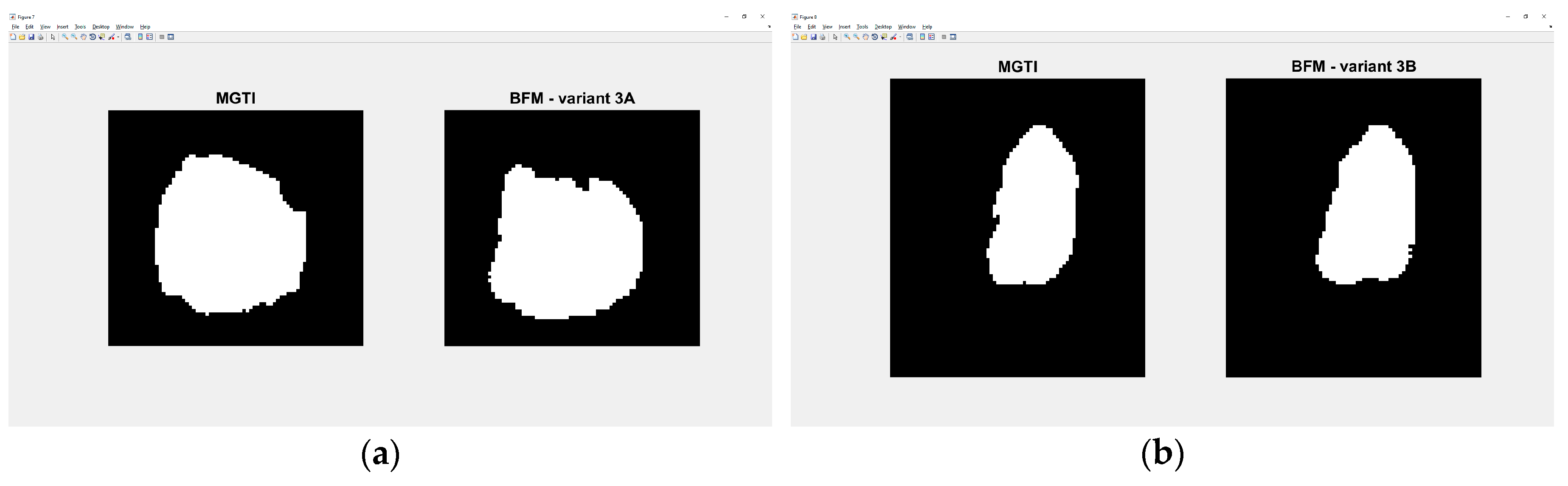
Symmetry 12 00416 g007
Figure 8. Generic diagram of the complete process.
Symmetry 12 00416 g008
Figure 9. Generic diagram of GGTI DL variants 1A−2B.
Symmetry 12 00416 g009
Figure 10. Generic diagram of GGTI DL variants 3A and AB.
Symmetry 12 00416 g010
Figure 11. (a) Training block for variant 1A. (b) Training block for variant 1B. (c) Training block for variant 2A and 3A. (d) Training block for variant 2B and 3B.
Symmetry 12 00416 g011
Figure 12. Diagram of software framework. It presents software implementation of modules, as well as inputs and outputs.
Symmetry 12 00416 g012
Figure 13. (a) Global GUI contains links to all other important GUI elements, as well as some other additional options and helpers. (b) GUI for MGTI—Module 1. (c) GUI for GGTI AP7—Module 2. (d) GUI (in usage) for variants 1A, 1B, 2A and 2B—Module 3.
Symmetry 12 00416 g013aSymmetry 12 00416 g013b
Figure 14. (a) GUI for GGTI DL variants 3A and 3B—Module 3. (b) Module 4 GUI offers load and preview of referenced, segmented and original slice, as well as export to MAT/TIFF data types, etc. (c) The second Module 4 GUI offers calculation of all metrics. (d) The GUI for batch 3D segmentation and evaluation.
Symmetry 12 00416 g014
Figure 15. Diagram results for variant 1A; Table 2, Table 3, Table 4 and Table 5.
Symmetry 12 00416 g015
Figure 16. Diagram results for variant 1B; Table 6, Table 7, Table 8 and Table 9.
Symmetry 12 00416 g016
Figure 17. Diagram results for variant 2A—Table 10, Table 11, Table 12 and Table 13.
Symmetry 12 00416 g017
Figure 18. Diagram results for variant 2B; Table 14, Table 15, Table 16 and Table 17.
Symmetry 12 00416 g018
Figure 19. Diagram results for variant 3A; Table 18, Table 19, Table 20 and Table 21.
Symmetry 12 00416 g019
Figure 20. Diagram results for variant 3B—Table 22, Table 23, Table 24 and Table 25.
Symmetry 12 00416 g020
Figure 21. (a) Sample image/slice of BBBC039 dataset. (b) Sample image/slice of BBBC035 dataset.
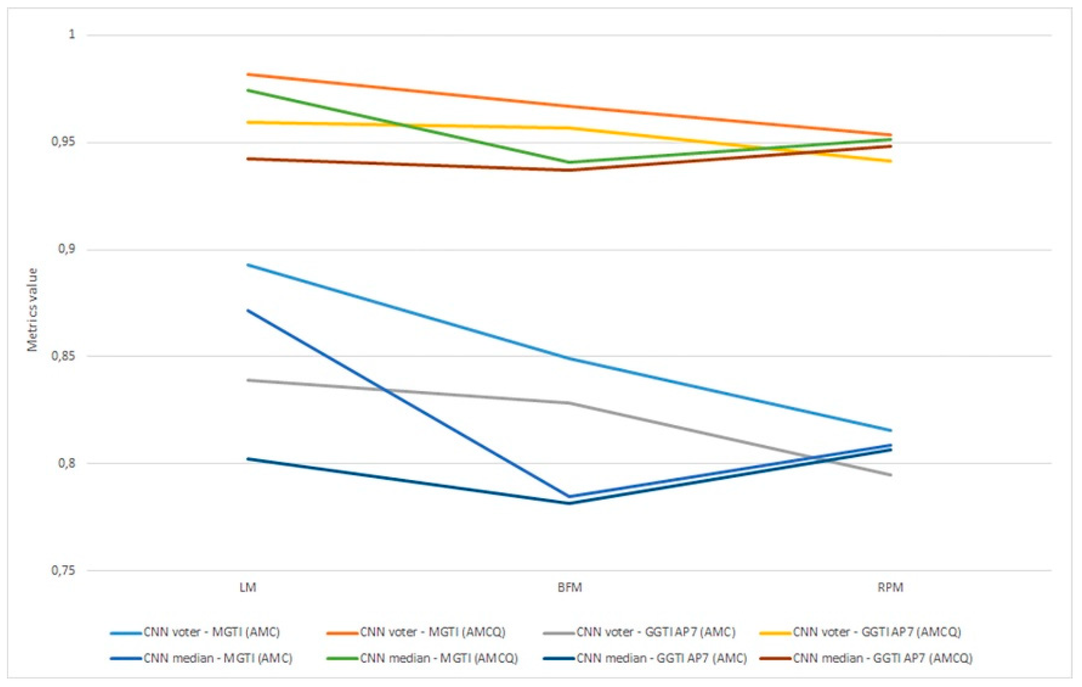
Symmetry 12 00416 g021
Figure 22. (a) Experiment 1-6, results for LPM method and AMCQ metrics. (b) Experiment 1-6, results for BFM method and AMCQ metrics. (c) Experiment 1–6, results for RPM method and AMCQ metrics.
Symmetry 12 00416 g022aSymmetry 12 00416 g022b
Figure 23. (a) Variant 1A—segmented slice of MGTI and LM CNN voter. (b) Variant 1B—segmented slices of MGTI and LM CNN voter.
Symmetry 12 00416 g023
Figure 24. (a) Variant 2A—segmented slices of MGTI and LM CNN voter. (b) Variant 2B—segmented slices of MGTI and LM CNN median.
Symmetry 12 00416 g024
Figure 25. (a) Variant 3A—segmented slice of MGTI and BFM CNN voter. (b) Variant 3B—segmented slices of MGTI and BFM CNN voter.
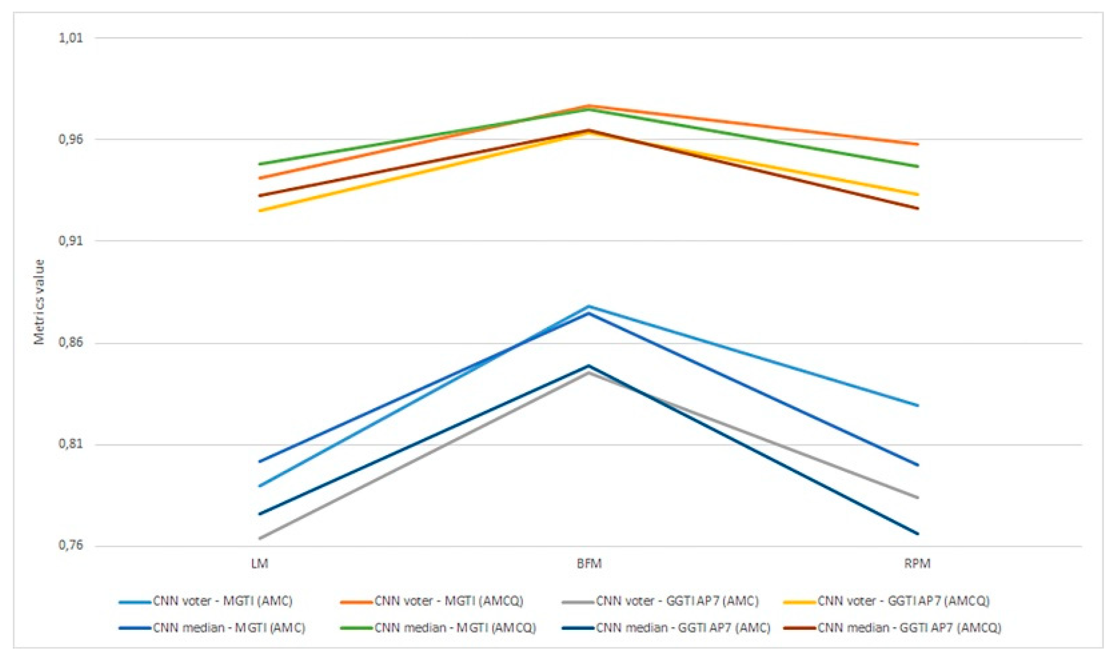
Symmetry 12 00416 g025
Figure 26. Experiment 7, results for six 3D stack samples and AMCQ metrics.
Symmetry 12 00416 g026
Figure 27. Segmentation of first and last five slices of Arabidopsis thaliana sample 1. GGTI AP7 is not having controlled segmentation over darker slices of samples, while GGTI DL gives controlled and reliable segmentation.
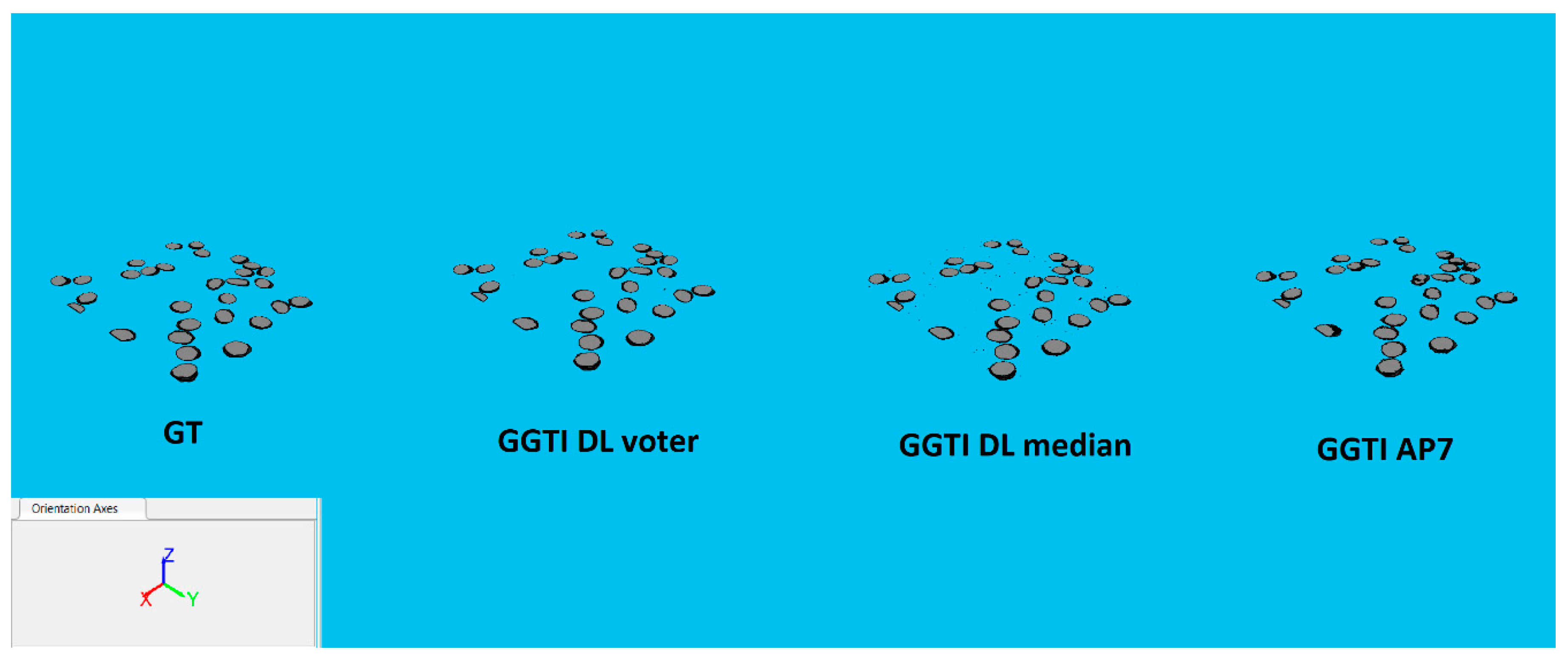
Symmetry 12 00416 g027
Figure 28. 3D segmentations of sample 4: MGTI, GGTI DL CNN voter, GGTI DL CNN median and GGTI AP7.
Symmetry 12 00416 g028
Figure 29. Experiment 8, results for all generalization variants and AMCQ metrics.
Symmetry 12 00416 g029
Figure 30. 3D segmentations of BBBC039 testing sample: GT, GGTI DL CNN voter, GGTI DL CNN median and GGTI AP7.
Symmetry 12 00416 g030
Figure 31. 3D segmentations of BBBC035 testing sample: GT, GGTI DL CNN voter, GGTI DL CNN median and GGTI AP7.
Symmetry 12 00416 g031
Table 1. Preview of variants 1A–3B.
VariantTraining Usage of Pre-Trained CNNsSemantic Segmentation—Validation
Number of Slices Per 3D Stack SampleNumber of 3D Stack Samples
Variant 1A11NoValidation slice belongs to training 3D stack sample, different than training slice.
Variant 1B1>1NoValidation slice belongs to 3D stack sample that has not been used in training.
Variant 2A>11NoValidation slice belongs to training 3D stack sample, different than training slices.
Variant 2B>1>1NoValidation slice belongs to 3D stack sample that has not been used in training.
Variant 3A>11Yes—from variant 2AValidation slice belongs to training 3D stack sample, different than training slices.
Variant 3B>1>1Yes—from variant 2BValidation slice belongs to 3D stack sample that has not been used in training.
Table 2. Results for variant 1A—CNN voter compared to MGTI.
MetricsLMBFMRPM
AMC0.880780.833610.84929
AMCQ0.976830.958120.96392
Table 3. Results for variant 1A—CNN voter compared to GGTI AP7.
MetricsLMBFMRPM
AMC0.823000.764980.76699
AMCQ0.952210.920900.92143
Table 4. Results for variant 1A—CNN median compared to MGTI.
MetricsLMBFMRPM
AMC0.840170.844680.84664
AMCQ0.963530.963400.96325
Table 5. Results for variant 1A—CNN median compared to GGTI AP7.
MetricsLMBFMRPM
AMC0.811290.783470.76811
AMCQ0.950340.931910.92203
Table 6. Results for variant 1B—CNN voter compared to MGTI.
MetricsLMBFMRPM
AMC0.878350.873160.87280
AMCQ0.976280.974840.97476
Table 7. Results for variant 1B—CNN voter compared to GGTI AP7.
MetricsLMBFMRPM
AMC0.852120.844500.84727
AMCQ0.964930.962390.96397
Table 8. Results for variant 1B—CNN median compared to MGTI.
MetricsLMBFMRPM
AMC0.878570.863070.86438
AMCQ0.976390.970830.97116
Table 9. Results for variant 1B—CNN median compared to GGTI AP7.
MetricsLMBFMRPM
AMC0.853510.849030.85025
AMCQ0.965490.964720.96522
Table 10. Results for variant 2A—CNN voter compared to MGTI.
MetricsLMBFMRPM
AMC0.893080.849200.81585
AMCQ0.981590.966680.95337
Table 11. Results for variant 2A—CNN voter compared to GGTI AP7.
MetricsLMBFMRPM
AMC0.838800.828220.79492
AMCQ0.959490.956940.94158
Table 12. Results for variant 2A—CNN median compared to MGTI.
MetricsLMBFMRPM
AMC0.871300.784910.80887
AMCQ0.974290.940650.95123
Table 13. Results for variant 2A—CNN median compared to GGTI AP7.
MetricsLMBFMRPM
AMC0.8023650.781290.80637
AMCQ0.9425180.936900.94822
Table 14. Results for variant 2B—CNN voter compared to MGTI.
MetricsLMBFMRPM
AMC0.885640.878810.87008
AMCQ0.978790.976160.97308
Table 15. Results for variant 2B—CNN voter compared to GGTI AP7.
MetricsLMBFMRPM
AMC0.855520.842120.83191
AMCQ0.966290.960000.95552
Table 16. Results for variant 2B—CNN median compared to MGTI.
MetricsLMBFMRPM
AMC0.887280.878270.86879
AMCQ0.979120.975640.97283
Table 17. Results for variant 2B—CNN median compared to GGTI AP7.
MetricsLMBFMRPM
AMC0.863130.849810.83226
AMCQ0.969590.962980.95602
Table 18. Results for variant 3A—CNN voter compared to MGTI.
MetricsLMBFMRPM
AMC0.789640.877920.82941
AMCQ0.941420.976690.95796
Table 19. Results for variant 3A—CNN voter compared to GGTI AP7.
MetricsLMBFMRPM
AMC0.763920.845300.78378
AMCQ0.925260.963470.93344
Table 20. Results for variant 3A—CNN median compared to MGTI.
MetricsLMBFMRPM
AMC0.801830.874810.80027
AMCQ0.947860.974930.94680
Table 21. Results for variant 3A—CNN median compared to GGTI AP7.
MetricsLMBFMRPM
AMC0.776260.848620.76622
AMCQ0.932600.964780.92621
Table 22. Results for variant 3B—CNN voter compared to MGTI.
MetricsLMBFMRPM
AMC0.922810.933900.90248
AMCQ0.987830.990640.98234
Table 23. Results for variant 3B—CNN voter compared to GGTI AP7.
MetricsLMBFMRPM
AMC0.882020.889440.86098
AMCQ0.973560.975360.96547
Table 24. Results for variant 3B—CNN median compared to MGTI.
MetricsLMBFMRPM
AMC0.910940.916950.89490
AMCQ0.985500.986070.97895
Table 25. Results for variant 3B—CNN median compared to GGTI AP7.
MetricsLMBFMRPM
AMC0.883260.877480.86304
AMCQ0.975700.971870.96556
Table 26. Results for Sample 1—2012-12-21-crwn12-008_GC1 batch 3D segmentation - CNN voter, CNN median, GGTI AP7 and NucleusJ compared to MGTI.
MetricsGGTI DL Voter Compared to MGTIGGTI DL Median Compared to MGTIGGTI AP7 Compared to MGTINucleusJ Compared to MGTI
AMC0.792180.799830.852710.89196
AMCQ0.934500.940390.964550.97612
Table 27. Results for Sample 2—2012-12-21-crwn12-009_GC1 batch 3D segmentation - CNN voter, CNN median, GGTI AP7 and NucleusJ compared to MGTI.
MetricsGGTI DL Voter Compared to MGTIGGTI DL Median Compared to MGTIGGTI AP7 Compared to MGTINucleusJ Compared to MGTI
AMC0.805840.805200.937010.91979
AMCQ0.944480.944380.991650.98655
Table 28. Results for Sample 3—2012-12-21-crwn12-009_GC2 batch 3D segmentation - CNN voter, CNN median, GGTI AP7 and NucleusJ compared to MGTI.
MetricsGGTI DL Voter Compared to MGTIGGTI DL Median Compared to MGTIGGTI AP7 Compared to MGTINucleusJ Compared to MGTI
AMC0.842450.838380.925160.91983
AMCQ0.961100.959910.989070.98760
Table 29. Results for Sample 4—2013-01-23-col0-3_GC1 batch 3D segmentation - CNN voter, CNN median, GGTI AP7 and NucleusJ compared to MGTI.
MetricsGGTI DL Voter Compared to MGTIGGTI DL Median Compared to MGTIGGTI AP7 Compared to MGTINucleusJ Compared to MGTI
AMC0.897530.880320.857230.81302
AMCQ0.982000.977240.966040.94573
Table 30. Results for Sample 5—2013-01-23-col0-3_GC2 batch 3D segmentation - CNN voter, CNN median, GGTI AP7 and NucleusJ compared to MGTI.
MetricsGGTI DL Voter Compared to MGTIGGTI DL Median Compared to MGTIGGTI AP7 Compared to MGTINucleusJ Compared to MGTI
AMC0.878930.861410.899510.84845
AMCQ0.971820.966660.980870.95708
Table 31. Results for Sample 6—2013-01-23-col0-8_GC1 batch 3D segmentation - CNN voter, CNN median, GGTI AP7 and NucleusJ compared to MGTI.
MetricsGGTI DL Voter Compared to MGTIGGTI DL Median Compared to MGTIGGTI AP7 Compared to MGTINucleusJ Compared to MGTI
AMC0.916280.887570.929870.89224
AMCQ0.985250.976370.989280.97586
Table 32. Variant 1G—Results for dataset: BBBC039—Nuclei of U2OS cells in a chemical screen; GGTI DL/GGTI AP7 compared to GT.
MetricsGGTI DL Voter Compared to GTGGTI DL Median Compared to GTGGTI AP7 Compared to GT
AMC0.914550.911820.94410
AMCQ0.985680.985170.99341
Table 33. Variant 1G—Results for dataset: BBBC035—Simulated nuclei of HL60 cells; GGTI DL/GGTI AP7 compared to GT.
MetricsGGTI DL Voter Compared to GTGGTI DL Median Compared to GTGGTI AP7 Compared to GT
AMC0.944510.936260.92042
AMCQ0.991720.989700.98569
Table 34. Variant 2G—Results for dataset: BBBC039—Nuclei of U2OS cells in a chemical screen; GGTI DL/GGTI AP7 compared to GT.
MetricsGGTI DL Voter Compared to GTGGTI DL Median Compared to GTGGTI AP7 Compared to GT
AMC0.956880.955360.94410
AMCQ0.996160.995960.99341
Table 35. Variant 2G—Results for dataset: BBBC035—Simulated nuclei of HL60 cells; GGTI DL/GGTI AP7 compared to GT.
MetricsGGTI DL Voter Compared to GTGGTI DL Median Compared to GTGGTI AP7 Compared to GT
AMC0.934320.931330.92042
AMCQ0.988910.988300.98569
Table 36. Variant 3G—Results for dataset: BBBC039—Nuclei of U2OS cells in a chemical screen; GGTI DL/GGTI AP7 compared to GT.
MetricsGGTI DL Voter Compared to GTGGTI DL Median Compared to GTGGTI AP7 Compared to GT
AMC0.947540.946660.94410
AMCQ0.994440.994310.99341
Table 37. Variant 3G—Results for dataset: BBBC035—Simulated nuclei of HL60 cells; GGTI DL/GGTI AP7 compared to GT.
MetricsGGTI DL Voter Compared to GTGGTI DL Median Compared to GTGGTI AP7 Compared to GT
AMC0.913230.913950.92042
AMCQ0.983760.983920.98569

