1. Introduction and Motivation
The monotonicity of the hazard (failure) rate function (HRF) of a life model plays an important role in modeling failure time data. Probability distributions with an increasing failure rate (IFR) have various applications in pricing and supply chain contracting studies. The IFR property is a well-known and useful concept in reliability theory, dynamic programming, and other areas of applied probability and statistics (See [
1,
2]). Recently, [
3] introduced a new two-parameter lifetime model with IFR. The model of [
3] is named the binomial-exponential
(BE-2) model, which is constructed as the distribution of the random sum (RSum) of independent exponential random variables (IID RVs) when the sample size (
) has a zero truncated binomial (ZTB) model. The BE-2 distribution can be used as an alternative to the standard Weibull (W), standard gamma (Ga), exponentiated exponential (EE), and weighted exponential (WhE) distributions. The cumulative distribution function (CDF) of BE-2 distribution is given by:
where
is the scale parameter, and
is the shape parameter, where
. The probability density function (PDF) corresponding to (1) can be expressed as:
The PDF in (1) can be written as:
where
. The BE-2 distribution is a mixture of the exponential (E) distribution (with scale parameter
), and the Ga distribution (with shape parameter
and scale parameter
), with mixing proportion
. We notice that when
we get the standard exponential distribution, and when
the BE-2 distribution reduces to the gamma distribution with shape parameter
and scale parameter
. The BE-2 distribution has a PDF whose shape is like those of Ga, W, WhE, and EE distributions.
Recently, [
4] proposed a general family of distributions called the Marshall–Olkin (MO-G) family of distributions. The MO-G family of distributions is also known as the proportional odds (PO) family. The CDF of the MO-G family is defined by:
The survival function (SF)
is given by:
where
, for
, we get the baseline model, i.e.;
, where the shape parameter
is called the tilt parameter. The PDF corresponding to (4) can be expressed as:
and the HRF is given by:
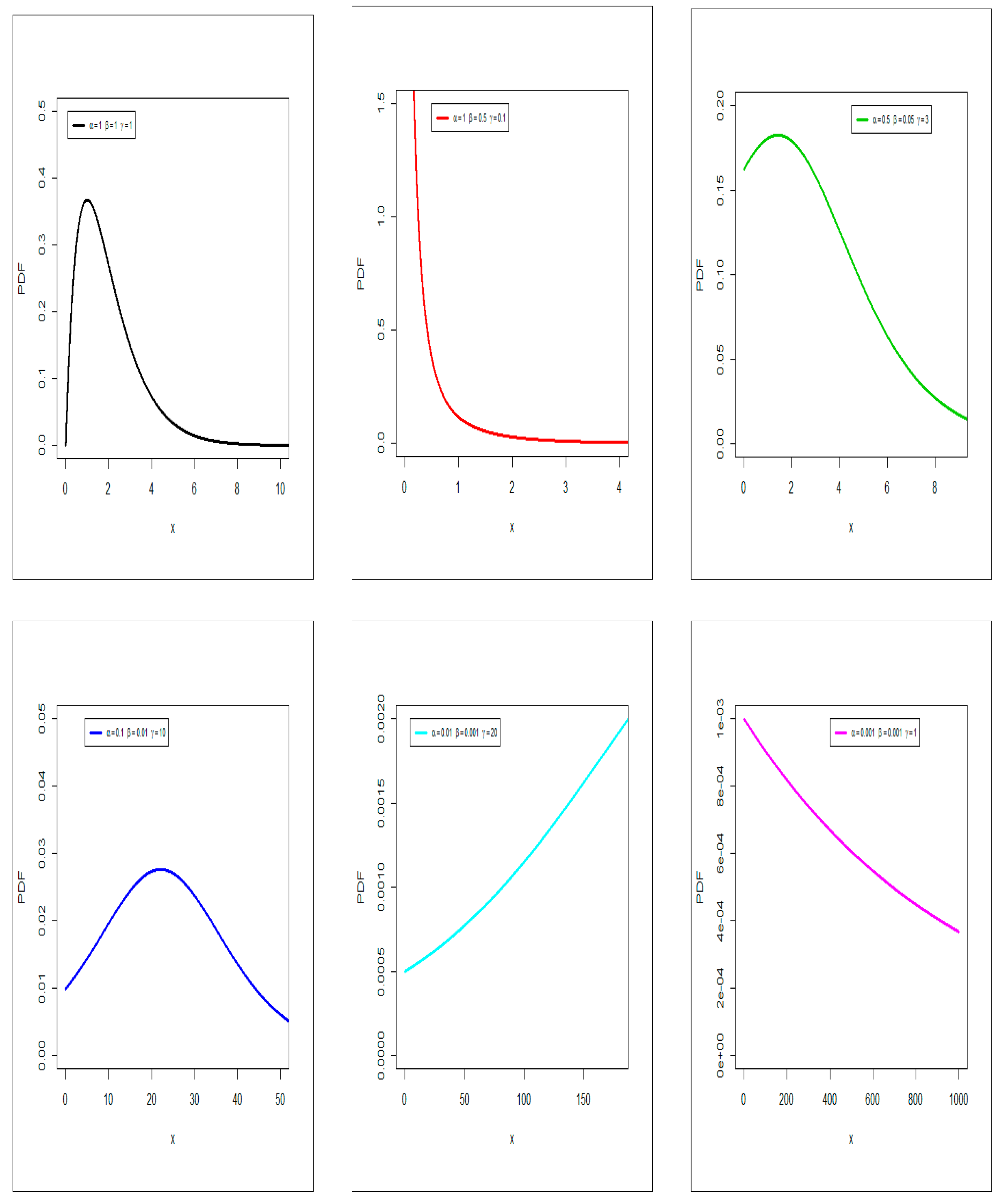
The new PDF of the proposed lifetime model distribution can be right-skewed, symmetric, and left-skewed with many different useful shapes (see
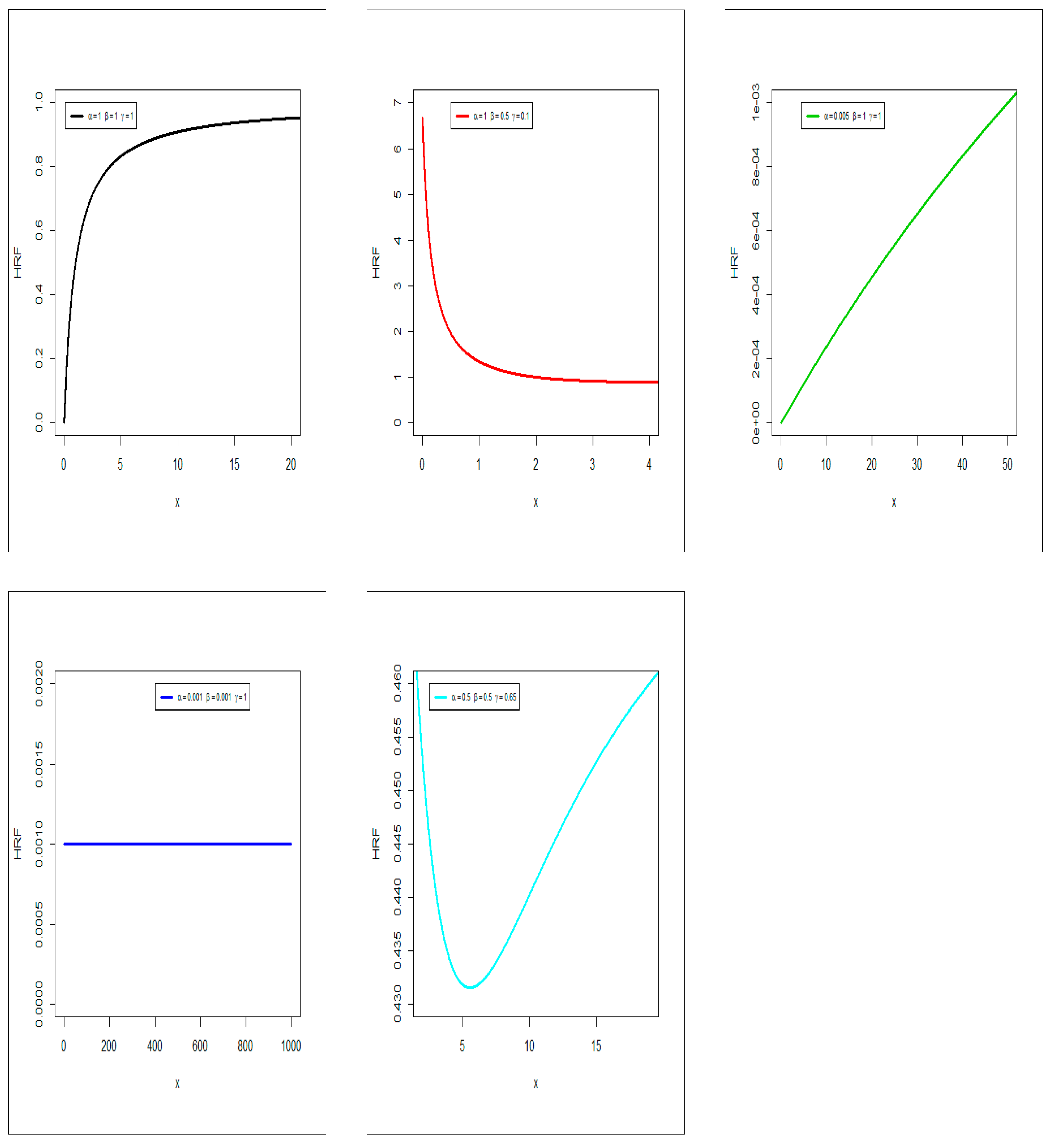
Figure 1), and this means that the new model will be suitable for modeling different real data sets, and the HRF of the new model exhibits many important HRF shapes such as the “increasing-constant”, “decreasing”, “increasing”, “constant”, and “bathtub” shapes (see
Figure 2).
Practically, the proposed lifetime model is much better than many competitive versions of the exponential model, such as the odd Lindley exponential, the Marshall–Olkin exponential, moment exponential, the logarithmic Burr–Hatke exponential, the generalized Marshall–Olkin exponential, beta exponential, the Marshall–Olkin–Kumaraswamy exponential, the Kumaraswamy exponential, and the Kumaraswamy–Marshall–Olkin exponential, so the new lifetime model may be a good alternative to these models in modeling relief times and survival times data sets.
2. Genesis of the New Model
In this section, we introduce the three parameters of the MOBE-2 distribution. Using (1) and (2) in Equations (4)−(6), we obtain the CDF, SF, and PDF of the MOBE-2 distribution, (for
) with vector of parameters
. The CDF and SF can be written as:
respectively. The corresponding PDF can be derived as:
Henceforth, let
MOBE-2
, with PDF (10). For the MOBE-2 distribution, the HRF can be written as:
The MOBE-2 distribution is a very flexible model that approaches different distributions when its parameters are changed. For
, the MOBE-2 distribution reduces to the Marshall–Olkin extended exponential (MOEE) distribution. For
, we get MOEGa distribution with shape parameter
and scale parameter
. For
, we get BE-2 distribution (see Bakouch et al. (2014)). For
and
, we get the exponential (E) distribution. For
, the MOBE-2 distribution reduces to the Ga model with shape parameter
and scale parameter
. A useful representation for the new PDF is given in
Appendix A.
Figure 1 below gives some plots of the new PDF based on some selected parameters values. Based on
Figure 1, we note that the new MOBE-2 distribution PDF can be right-skewed and left-skewed with many different useful shapes.
Figure 2 below gives some plots of the new HRF based on some selected parameters values. From
Figure 2 we note that the HRF of the new model exhibits many important HRF shapes, such as the increasing-constant
, decreasing
, increasing
, constant
, and bathtub
shapes.
The solution of the following relationship is used to find the quantile function (QF) of the MOBE-2 distribution, as follows:
Since the uniform RVs are easily generated numerically in most statistical packages, the above scheme in (12) is very useful to generate MOBE-2 RVs and therefore can be easily implemented. It facilitates ready quantile-based statistical modeling. In particular, the median of
is
, given by setting
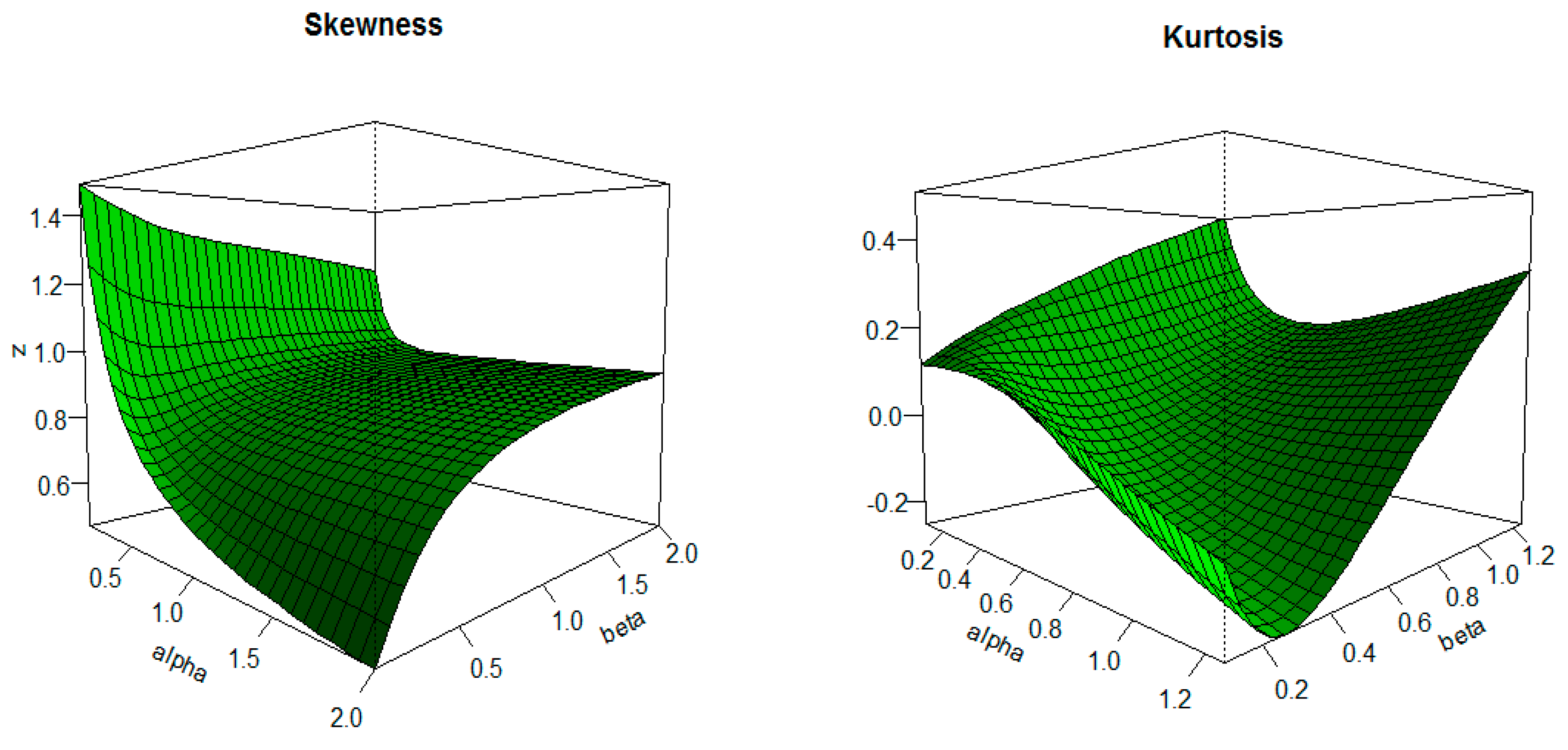
in (12). Also using (12), we can determine the Bowley’s skewness and the Moors’ kurtosis. The Bowley’s skewness is based on quartiles.
Figure 3 indicates that both measures depend very much on the shape parameters
.
6. Modeling
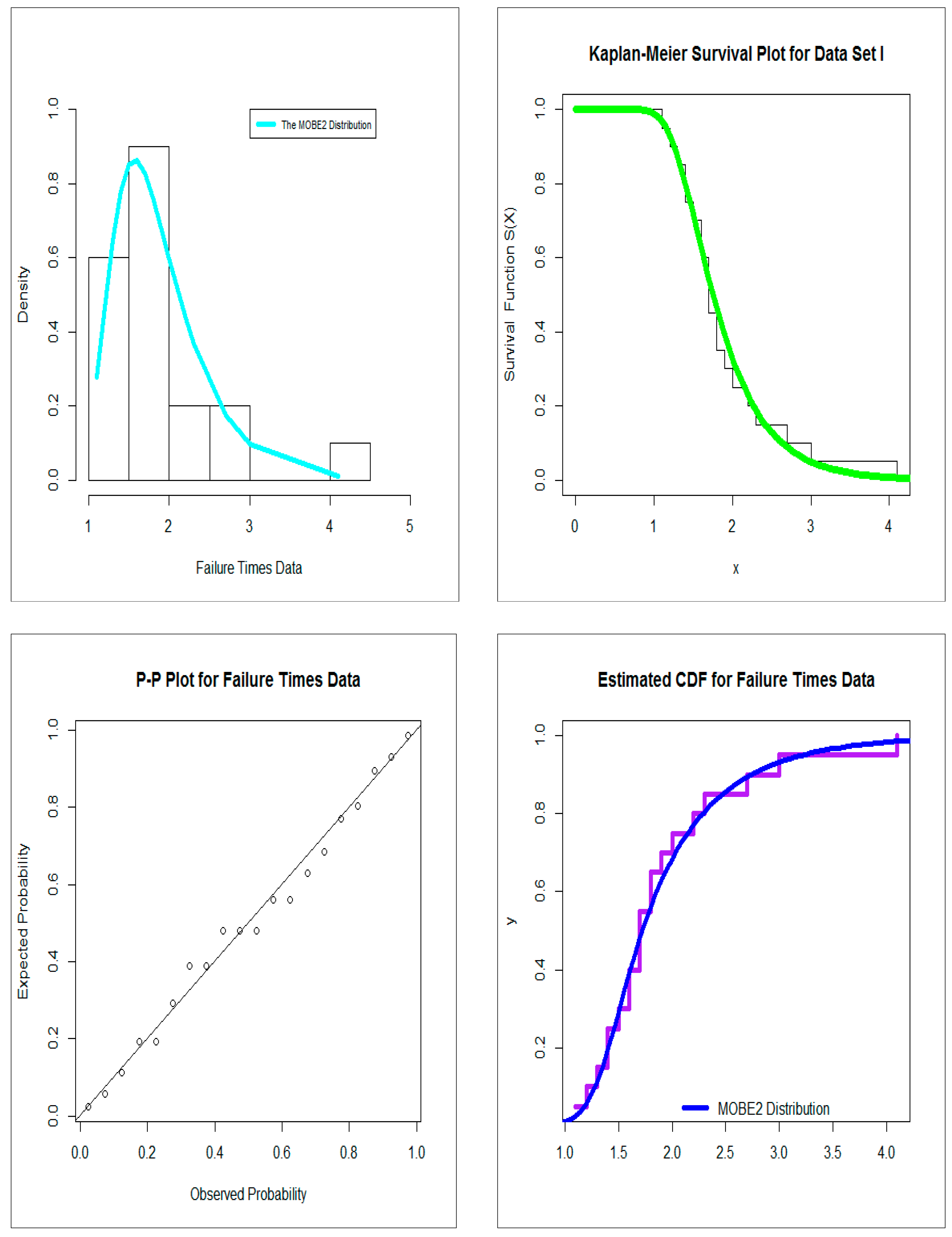
In this Section, two real data applications are presented for illustrating the importance and flexibility of the new model. The first data set (1.1, 1.4, 1.3, 1.7, 1.9, 1.8, 1.6, 2.2, 1.7, 2.7, 4.1, 1.8, 1.5, 1.2, 1.4, 3, 1.7, 2.3, 1.6, 2), called the failure time data, represents the lifetime data relating to relief times (in minutes) of patients receiving an analgesic (for more applications to this data see [
6,
7,
8,
9,
10,
11,
12]).
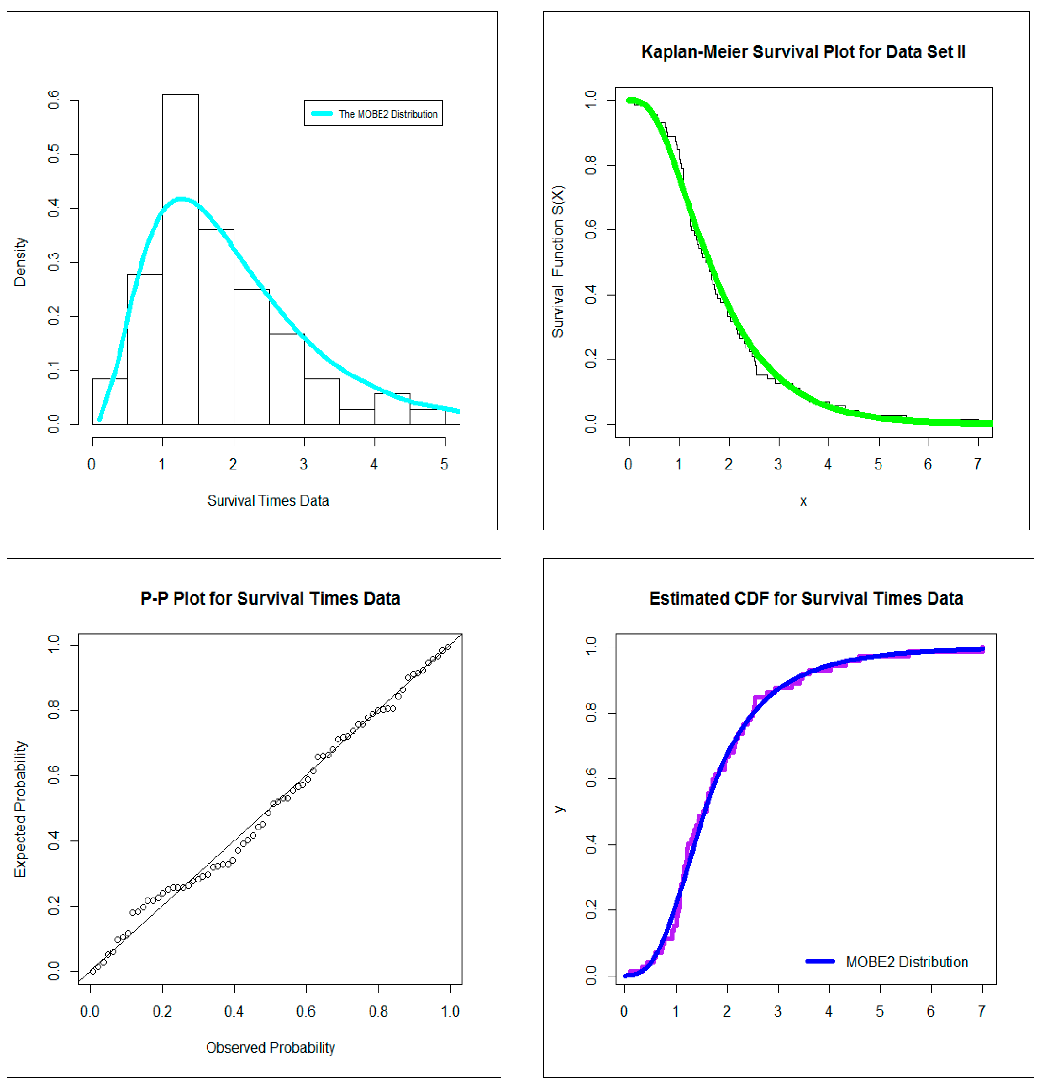
The second data set (0.1, 0.33, 0.44, 0.56, 0.59, 0.72, 0.74, 0.77, 0.92, 0.93, 0.96, 1, 1, 1.02, 1.05, 1.07, 07, 1.08, 1.08, 1.08, 1.09, 1.12, 1.13, 1.15, 1.16, 1.2, 1.21, 1.22, 1.22, 1.24, 1.3, 1.34, 1.36, 1.39, 1.44, 1.46, 1.53, 1.59, 1.6, 1.63, 1.63, 1.68, 1.71, 1.72, 1.76, 1.83, 1.95, 1.96, 1.97, 2.02, 2.13, 2.15, 2.16, 2.22, 2.3, 2.31, 2.4, 2.45, 2.51, 2.53, 2.54, 2.54, 2.78, 2.93, 3.27, 3.42, 3.47, 3.61, 4.02, 4.32, 4.58, 5.55) represents the survival times (in days) of 72 guinea pigs infected with virulent tubercle bacilli, observed and reported by Bjerkedal (1960). Many other real data sets related to failure times can be found in [
13,
14,
15,
16,
17,
18,
19,
20].
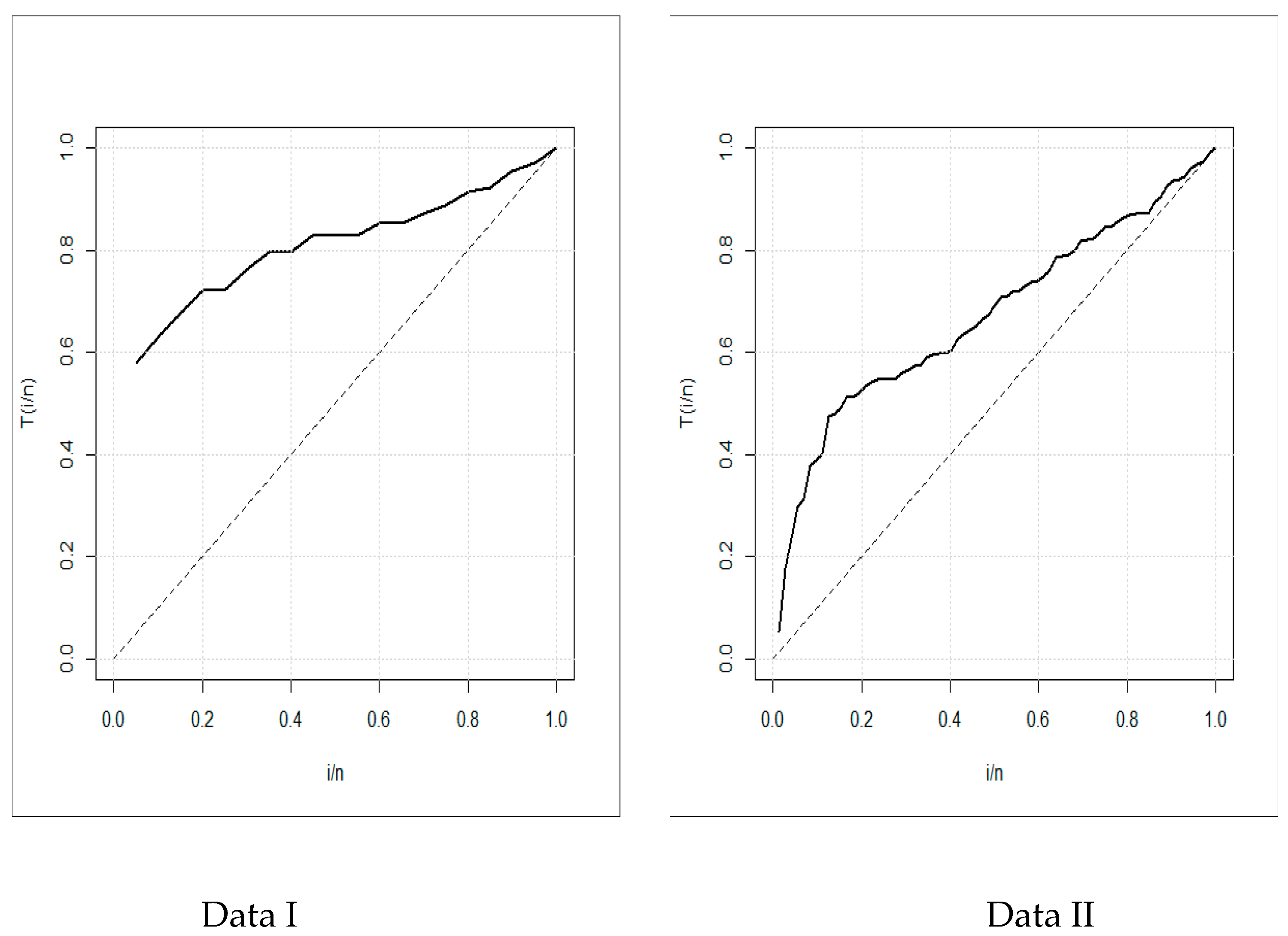
Figure 3 gives the total time test (TTT) plots.
Figure 4 and
Figure 5 gives the estimated PDF (EPDF), estimated survival function (ESF), P-P plots, and estimated CDF (ECDF) for the two data sets, respectively. From
Figure 3, we note that the empirical HRF is increasing for the two data sets.
We compared the fits of the MOBE-2 distribution with some competitive models, namely: exponential (E
), odd Lindley exponential (OLiE), MO exponential (MOE
), moment exponential (MomE
), the logarithmic Burr–Hatke exponential (Log BrHE
), generalized MO exponential (GMOE
), beta exponential (BE
), MO–Kumaraswamy exponential (MOKwE
), Kumaraswamy exponential (KwE
), and Kumaraswamy MO exponential (KwMOE
). See the PDFs of the competitive moels in [
21,
22,
23,
24,
25,
26,
27,
28,
29,
30,
31]. We considered the Cramér-Von Mises (
), the Anderson–Darling (
), and the Kolmogorov–Smirnov (KS) statistics. The
and
statistics are given by:
and:
where:
and:
where
and
’s values are the ordered observations. Moreover, we considered some other goodness-of-fit measures, including the Akaike Information Criterion (AIC), Consistent Akaike Information Criterion (CAIC), Hannan–Quinn Information Criterion (HQIC), and Bayesian Information Criterion (BIC).
Table 1 gives the maximum likelihood estimations (MLE) and SE values for the relief times data.
Table 2 give the AIC, BIC, CAIC, and HQIC for the relief times data.
Table 3 gives
,
, KS, and
p-value for the relief times data.
Table 4 gives the MLE and SE values for the survival times data.
Table 5 gives the AIC, BIC, CAIC, and HQIC for the survival times data.
Table 6 gives the
,
, KS, and
p-value for the survival times data.
Based on
Table 2,
Table 3,
Table 5 and
Table 6, the proposed lifetime MOBE-2 model is much better than many competitive models, such as the E, MomE, MOE, GMOE, KwE, BE, MOKE, and KMOE models, so the new lifetime model may be a good alternative to these models in modeling relief times and survival times data sets. From
Figure 5 and
Figure 6, we note that the MOBE-2 model gives an adequate fit with the two real data sets.


