Brain Extraction Using Active Contour Neighborhood-Based Graph Cuts Model

Abstract

The extraction of brain tissue from brain MRI images is an important pre-procedure for the neuroimaging analyses. The brain is bilaterally symmetric both in coronal plane and transverse plane, but is usually asymmetric in sagittal plane. To address the over-smoothness, boundary leakage, local convergence and asymmetry problems in many popular methods, we developed a brain extraction method using an active contour neighborhood-based graph cuts model. The method defined a new asymmetric assignment of edge weights in graph cuts for brain MRI images. The new graph cuts model was performed iteratively in the neighborhood of brain boundary named the active contour neighborhood (ACN), and was effective to eliminate boundary leakage and avoid local convergence. The method was compared with other popular methods on the Internet Brain Segmentation Repository (IBSR) and OASIS data sets. In testing cross IBSR data set (18 scans with 1.5 mm thickness), IBSR data set (20 scans with 3.1 mm thickness) and OASIS data set (77 scans with 1 mm thickness), the mean Dice similarity coefficients obtained by the proposed method were 0.957 ± 0.013, 0.960 ± 0.009 and 0.936 ± 0.018 respectively. The result obtained by the proposed method is very similar with manual segmentation and achieved the best mean Dice similarity coefficient on IBSR data. Our experiments indicate that the proposed method can provide competitively accurate results and may obtain brain tissues with sharp brain boundary from brain MRI images.

1. Introduction

Brain extraction or skull stripping is needed before most of neuroimaging analyses, such as registration between MRI images [1,2,3], measurement of brain volume [4,5], brain tissue classification [6], and cortical surface reconstruction [7]. During recent years, automatic or semi-automatic brain extraction techniques have become the choices for fast brain extraction. These techniques can generally be categorized into three types: region-based [8,9,10], boundary-based [2,6,7,11,12], and hybrid methods [13,14,15,16,17,18,19,20].

The region-based methods first use thresholding or clustering techniques to divide brain MRI image into several regions by considering that the voxels in the same tissue have similar intensities, and then the brain region can be extracted from these regions by morphological operations or region merging. These thresholding or clustering techniques frequently used in brain extraction are Gaussian mixture model [8], intensity thresholding [9] and watershed algorithm [10]. The parameters in the region-based methods have remarkable effects on the brain extraction and need to be determined properly [12].

The boundary-based methods partition the brain MRI image into internal part (brain) and external part (non-brain) by detecting the boundary between brain and non-brain tissues. Smith [2] proposed a Brain Extraction Tool (BET) by using smoothing and pushing forces to push a tessellated mesh to the brain boundary. Shattuck et al. [6] proposed the Brain Surface Extraction (BSE) method by using a Marr–Hildreth edge detector to separate brain and non-brain tissues. The boundary-based methods [11,12] used active contour model that has made great progress in medical image segmentation during recent years.

The hybrid methods try to use a two steps strategy to improve the extraction result. In the first step, a rough brain region or boundary is obtained to be the initial brain region or boundary in the next step. Next, the brain contour or region is refined to get a more accurate result since it is close to the brain boundary at the first stage. Huang et al. [13] employed the expectation maximization algorithm on a mixture of Gaussian models to determine the initial brain contour for the geodesic active contour evolution. Ségonne et al. [14] proposed a hybrid watershed algorithm (HWA) applying the watershed algorithm to get an initial brain volume for deformable brain mesh. Sadananthan et al. [15] used graph cuts based image segmentation to refine the preliminary binary mask generated by intensity thresholding. Jiang et al. [16] used BET to generate the initial brain boundary, and then refined the brain boundary using a hybrid level set model.

To improve the robustness, some hybrid-based methods warp the brain volume to an atlas using registration techniques before brain extraction, then use the parameter learning techniques such as meta-algorithm, random forest and neural networks to get the proper initial region or parameters to perform brain extraction. Wang et al. [17] warped an atlas to the brain volume to obtain the initial brain mask, and then refined the mask with a deformable-surface similar with BET. Iglesias et al. [18] proposed a robust, learning-based brain extraction system (ROBEX). ROBEX used a trained random forest classifier to detect the brain boundary. Then the contour was refined to obtain the final brain tissues using graph cuts. Eskildsen et al. [19] proposed an atlas-based method with nonlocal segmentation technique, without the need of time-consuming non-rigid registrations. Huang et al. [20] used a trained Locally Linear Representation-based Classification (LLRC) method for brain extraction. By using registration techniques, the atlas-based methods can address the problem of variability in anatomy and modality and produce more robust results. However, the registration in atlas-based methods is usually highly time-consuming and if the registration fails, bad result may be obtained.

In recent years, the deep learning techniques were used for brain extraction. Kleesiek et al. [21] used a 3D convolutional neural network for brain extraction. Saleh et al. [22] applied U-Net for brain extraction. However, the output of these learning-based brain extraction method tends to be over-smoothed if the training data are obtained by automatic brain extraction method under the checking by human experts or by weak bounding box labeling [23]. In other words, if we want the learning-based brain extraction method to output brain tissue with sharp boundary, the training data should be quite precise and be obtained by manual. For example, Hwang et al. [24] recently applied 3D U-Net for brain extraction and achieved high extraction accuracy by using a fine training data.

Although the above methods have greatly improved the accuracy and robustness for brain extraction, these methods can not completely substitute for manual method for the appearances of over-smoothness, leakage through a weak boundary and missing brain tissues caused by local convergence. Unfortunately, it is a conflicting problem to improve all of them. Brain extraction is a compromised problem where a semi-global understanding of the image is required as well as a local understanding [2]. For example, it is effective that we use local region features to obtain sharp brain boundary and eliminate the leakage, but it is easy to lead to local convergence at the edges between the white matter and gray matter if the initial region is far from the true brain boundary. Trying to address these problems, we proposed a new brain extraction method from T1-weighted MRI volume. The main contributions of our work can be summarized as follows:

1. We defined a new asymmetric assignment of edge weights in graph cuts for brain MRI image to obtain brain boundary.

2. We performed the new graph cuts model iteratively in the neighborhood of brain boundary named the active contour neighborhood (ACN), and the new model was effective to eliminate boundary leakage and avoid local convergence.

3. By the asymmetric function of edge weights, we reduced the edge weights in the region between the ACN and the region in the current boundary to obtain a sharp brain boundary.

The remainder of this paper is organized as follows. In Section 2, the details of the designed brain extraction method including the ACN and graph cuts are introduced. In Section 3, experiments and results are presented. Finally, we give a detailed discussion on the analysis of our experiments in Section 4.

2. Materials and Methods

2.1. Data Sets

To measure the extraction accuracy of our method, we used the following three data sets:

1. Data set 1 (IBSR18): 18 normal T1-weighted MR Image data sets with expert segmentations from IBSR. Each volume has around 128 coronal slices, with 256 × 256 pixels per slice and 1.5mm thickness.

2. Data set 2 (IBSR20): 20 normal T1-weighted MR Image data sets from IBSR, with 256 × 256 pixels per coronal slice and 3.1 mm thickness. Obvious intensity inhomogeneity and other significant artifacts present in most of the MR images in this data set. Another challenge of this data set is that the neck and even shoulder areas are included.

3. Data set 3 (OASIS77): 77 T1-weighted MR Image data sets were obtained from OASIS project. Each volume has around 208 coronal slices, with 176 × 176 pixels per slice and 1mm thickness. The brain masks for this set were obtained by an atlas-based brain extraction method automatically, checked by human experts before releasing the data. Although the lack of exactitude makes it unfit for testing the precision of a method, we can use it to test the robustness of a method because it includes scans from a very diverse population with a very wide age range as well as diseased brains [19].

We downloaded IBSR data sets from https://www.nitrc.org/projects/ibsr and OASIS77 data set from http://www.oasis-brains.org/ by agreeing the license agreements to access all the data sets.

2.2. Graph Cuts

In our previous work [16] we used BET to pre-process T1-weighted MRI scans to generate a robust initial contour and obtained the active contour neighborhood (ACN) [25] by dilating the contour with a small size. In this paper, we used a modified graph cuts to refine the brain contour in ACN. Thus, the ACN and brain contour can be obtained iteratively. Since the initial contour obtained by BET is close to the real brain boundary, the real brain boundary should be the global minimum within the ACN obtained by the initial contour, and the redefined edge weights are more powerful than GCUT [15] for brain extraction.

The graph cuts approaches [26,27,28,29] model the image as a weighted undirected graph $𝒢$ = ($𝒱$, $ℰ$, $𝒲$), where $𝒱$, $ℰ$ and $𝒲$ are sets of vertices, edges and edge weights respectively. Let A = (A₁,...,A_p,..., A_|$𝒫$|) be a binary vector whose components A_p specify assignments to pixels p in data set $𝒫$. Each A_p can be either “obj” or “bkg” (abbreviations of “object” and “background”). In the graph described by Boykov and Jolly [26], an energy function was defined as below:

$$E(A)=\lambda R(A)+B(A)$$

(1)

$$R(A)=\sum _{p\in \mathcal{P}}{R}_p(A_p)$$

(2)

$$R_p(“\mathrm{obj}”)=-\ln \mathrm{Pr}(I_p|\mathcal{O})$$

(3)

$$R_p(“\mathrm{bkg}”)=-\ln \mathrm{Pr}(I_p|\mathcal{B})$$

(4)

where R(A) is the regional term and B(A) is the boundary term. R_p(“obj”) and R_p(“bkg”) reflect how the intensity of the pixel p fits the histogram of the object ($𝒪$) and background ($ℬ$) models respectively. The boundary term B(A) was described by:

$$B(A)={\displaystyle \sum _{p,q\in \mathcal{N}}B\left\{p,q\right\}\cdot \delta (A_p,A_q)}$$

(5)

where

$$\delta (A_p,A_q)=\{\begin{array}{l}1 A_p\ne A_q\\ 0 \mathrm{otherwise}\end{array}$$

(6)

A well-known Min-Cut/Max-Flow algorithm can be used to minimize the energy function, and the cut will separate the image into deferent regions. Usually, the graph $𝒢$ = ($𝒱$, $ℰ$, $𝒲$) has two special vertices (terminals), namely, the source $𝒮$ and the sink $𝒯$. Let {p, q} be the two vertices in the graph and $𝒩$ be the neighbors of them. The edge weights between all the vertices in the graph are described in

Table 1. The edge weights in the graph.

Edge	Weight	for
$\{p,q\}$	$B\{p,q\}$	$\{p,q\}\in \mathcal{N}$
$\{p,\mathcal{S}\}$	$\lambda R_p(“\mathrm{bkg}”)$	$p\in \mathcal{P},p\notin \mathcal{O}\cup \mathcal{B}$
	K	$p\in \mathcal{O}$
	0	$p\in \mathcal{B}$
$\{p,\mathcal{T}\}$	$\lambda R_p(“\mathrm{obj}”)$	$p\in \mathcal{P},p\notin \mathcal{O}\cup \mathcal{B}$
	0	$p\in \mathcal{O}$
	K	$p\in \mathcal{B}$

.

where

$$K=1+\underset{p\in \mathcal{P}}{\max }\sum _{q:\{p,q\}}B\{p,q\}$$

(7)

2.3. Active Contour Neighborhood-Based Graph Cuts Model

To address the over smoothness, boundary leakage and asymmetry problem, we used a piecewise function to define the edge weights in graph cuts, which was more powerful than GCUT. To avoid local convergence, we performed graph cuts in ACN.

2.3.1. Description of ACN Model (ACNM)

The elements of the pipeline for the ACN model are shown in Figure 1. The first step is to obtain a rough boundary by a modified BET method for 2D images [30] from a round initial contour. Although the rough boundary is too smooth, it is close to the brain tissue and is still fit well for providing a good initial contour for brain extraction, due to the good robustness of BET. Then, the ACN is obtained by dilating the rough boundary. In the ACN, a graph cuts model is defined and performed to obtain a new boundary. Finally, a more accurate and sharper brain boundary is obtained by iteratively replacing the new boundary and the ACN. The maximum iteration number in Figure 1 was 10 in this paper.

2.3.2. Edge Weights Assignment in ACNM

In the defined graph cuts model for brain extraction, the edge weights between all the vertices in the graph are described in

Table 2. The edge weight in the graph used in ACN.

Edge	Weight	for
$\{p,q\}$	$B\{p,q\}$	$\{p,q\}\in \mathcal{N}$
$\{p,\mathcal{S}\}$	$\lambda R_p(“brain”)$	$p\in ACN$
	$\lambda \underset{p\in ACN}{\min }{R}_p(“brain”)$	$p\in \mathcal{O}$
	$\lambda \underset{p\in ACN}{\max }{R}_p(“brain”)$	$p\in \mathcal{B}$
$\{p,\mathcal{T}\}$	$\lambda R_p(“nonbrain”)$	$p\in ACN$
	$\lambda \underset{p\in ACN}{\max }{R}_p(“nonbrain”)$	$p\in \mathcal{O}$
	$\lambda \underset{p\in ACN}{\min }{R}_p(“nonbrain”)$	$p\in \mathcal{B}$

. The brain tissues and non-brain tissues are considered as the Object ($𝒪$) and Background ($ℬ$) respectively in our work, thus the ACN in Table 2 exactly corresponds to the area $p\in \mathcal{P},p\notin \mathcal{O}\cup \mathcal{B}$ in Table 1 (see in Figure 2). R(“brain”) and R(“nonbrain”) are the likelihood items reflecting how the vertex is fit for brain or non-brain tissues respectively. For ACN, we firstly classified the ACN into “brain” and “nonbrain” regions using Fuzzy C-Means clustering method (FCM) [31,32], then obtained the their likelihood items from Equation (3) and Equation (4). Recalling that $ℬ$ should include most of the non-brain tissues and inversely in $𝒪$, we simply set the edge weights between the terminal ($𝒮$ and $𝒯$) and vertex in $𝒪$ and $ℬ$ as the minimal or maximal value of R(“brain”) and R(“nonbrain”) in ACN respectively.

When setting the edge weights between the vertex and its neighbors ($𝒩$) B{p,q}, we used the following equations:

$$B\{p,q\}=D(p,q)\cdot G(p,q)\cdot R(p,q)$$

(8)

where

$$D(p,q)=\underset{p,q\in \mathcal{N}}{\max }\left[D_t(p),D_t(q)\right]$$

(9)

$$D_t(p)=\{\begin{array}{l}{k}_D\exp (\frac{2d_{pb}}{W}), p\in ACN\cap R_b\\ \exp (\frac{2d_{pb}}{W}), \mathrm{otherwize}\end{array}$$

(10)

$$G(p,q)=\underset{p,q\in \mathcal{N}}{\min }\left[I_G(p),I_G(q)\right]$$

(11)

$$I_G(p)=\{\begin{array}{l}\exp \left(k_0\frac{I(p)-\mu }{I_m-\mu }\right), I(p)-\mu >0\\ \exp \left(k_1\frac{\mu -I(p)}{I_m-\mu }\right), I(p)-\mu \le 0\end{array}$$

(12)

$$R(p,q)=\underset{p,q\in \mathcal{N}}{\max }\left[I_R(p),I_R(q)\right]$$

(13)

$$I_R(p)=\exp (2I_{\max })$$

(14)

$$I_{\max }=\max \left(t_m,I(0),I(1),\cdots ,I(d)\right)$$

(15)

Compared with the B{p,q} used in GCUT [15], we redefined the D(p,q) and G(p,q) in Equations (9)–(12) and added a new regional item R(p,q) in Equations (13)–(15).

In (10) $d_{pb}$ is the minimal distance between p and the current brain boundary, and W is the width of the image. This assignment increases the weight of edges locating deep within the foreground region, making cuts here less likely. $k_D$ is a parameter to control the smoothness. If over-smoothness occurs, a small $k_D$ can be selected to reduce the edge weights in the region between the ACN and $R_b$ (the region in the current boundary), and then the current brain boundary will move inside to touch the true brain boundary. The new G(p,q) in Equation (11) was defined by a piecewise function (12), which depends on the grayscale value of p, the mean grayscale value μ of the ACN and the maximal value $I_m$ of the ACN. The plot corresponding to Equation (12) is shown in Figure 3.

In Figure 3, $\mu =0.5$, $I_{\mathrm{m}}=0.9$, $k_0=6$ and $k_1=0.55k_0$, they control the range of the grayscale values that could be considered inside the brain tissues. Generally, the true brain boundary should locate rather on the vertices with grayscale values close to $\mu$ than on the vertices with lower or higher grayscale values. So, wherever $I(p)$ equals to $\mu$, we set $I_G(p)=1$ to make the voxels whose grayscale values are close to $\mu$ touched by the active contour. Wherever $I(p)\ne \mu$, we set $I_G(p)>1$ and the active contour will move away from the voxels whose grayscale values are far from $\mu$. Considering the true brain boundary more likely locates on the lower intensity side of the vertices whose grayscale values are close to $\mu$, we set $k_1=0.55k_0$. Thus, Equation (12) is a piecewise function, which is also well fit for the asymmetric distribution of intensity in the brain images.

The regional term R(p,q) in Equations (13)–(15) is used to eliminate boundary leakage trough the edge between the brain and eyeball. R(p,q) depends on the regional maximal value $I_{\max }$ which was firstly used in BET and then used by Zhuang et al. [11] and Liu et al. [12]. $I_{\max }$ is searched along a line pointing inward from the current vertex within a distance d. t_m is the median intensity of the brain tissue on each slice, which is approximated from the pixels within the initial brain region. $I_{\max }$ increases the edge weights on the eyeball to avoid the brain boundary leaking through the eyeball tissue.

3. Results

3.1. Evaluation Metrics

1. Similarity coefficients. We used Jaccard similarity, defined as $JS=\left|M\cap N\right|/\left|M\cup N\right|$, and Dice similarity, defined as $DS=2\left|M\cap N\right|/(\left|M\right|+\left|N\right|)$, where M and N refer to the extraction result and the ground truth respectively.

2. Segmentation error coefficients. We used False Positives Rate ($F{P}_{Rate}$) and False Negatives Rate ($F{N}_{Rate}$), defined as $F{P}_{Rate}=(\left|M\right|-\left|M\cap N\right|)/\left|N\right|$ and $F{N}_{Rate}=(\left|N\right|-\left|N\cap M\right|)/\left|N\right|$.

3. The recognizing rate (Sensitivity, SE) and rejecting rate (Specificity, SP). We used $SE=\left|M\cap N\right|/\left|N\right|$, and $SP=\left|I-M-N\right|/\left|I-N\right|$.

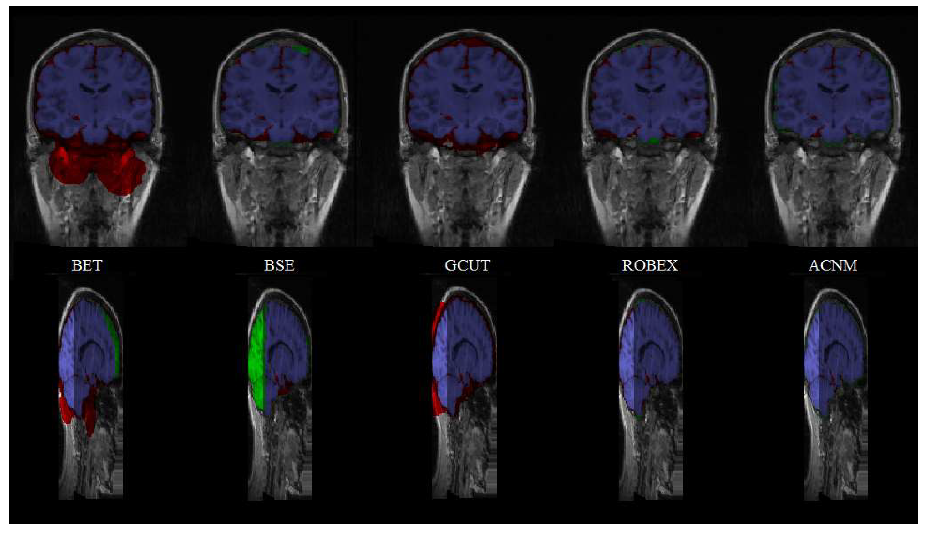
3.2. Comparison to Other Methods

Because BET, BSE, GCUT and ROBEX are all free and publicly available, a comparison to them was performed on the chosen data sets. The software of our work was programmed with matlab2016 and we tested it on a computer with 8GB RAM and Intel i7-4790 CPU. The software cost about 2 minutes to process one MRI volume on this computer. In this software, only two parameters $k_D$ and $k_0$ in Equation (10) and Equation (12) were needed to be set by the user for different volumes. $k_D$ is positively associated with the smoothness degree of brain boundary. $k_0$ is negatively associated with the average intensity of brain tissue. In testing, we chose $k_D=0.80$ and $k_0=5.5$ for IBSR18, $k_D=0.83$ and $k_0=1.2$ for IBSR20, $k_D=1$ and $k_0=6$ for OASIS77 to get the best results. The extremely low $k_0$ used in IBSR20 was to deal with the extremely high value and inhomogeneity of intensities in brain tissue. Before performing our method, the modified BET was done on the coronal middle slice once to obtain the initial contour. The initial contours of the other slices in the 3D volume were obtained by the resultant brain boundary of previous slice in a slice by slice manner, which was described in detail in our previous work [16]. The parameters of the BET were almost the same for all the data sets, which are quite easy to be set according to our previous work [30] for the robustness of BET. When estimating the centroid and the equivalent radius of the brain in BET, extra biases were added to them for IBSR20 because the images in IBSR20 include a lot of tissues in neck. For GCUT and ROBEX, we used the default parameters setting in their software. For BET and BSE, we used the different parameters on different volumes in the three data sets to obtain the best results by processing each volume for several times.

Table 3. Comparison of our method with BET, BSE, GCUT and ROBEX using IBSR18 Data Set.

Method	DS Mean (SD)	JS Mean (SD)	FPRATE (%) Mean (SD)	FNRATE (%) Mean (SD)
BET P*-value	0.946(0.012) 3.0 × 10−4	0.898(0.021) 3.3 × 10−4	8.36(2.77) 4.65 × 10−7	2.83(2.92) 1.09 × 10−4
BSE P*-value	0.943(0.039) 5.0 × 10−2	0.895(0.066) 4.87 × 10−2	7.82(6.20) 8.71 × 10−3	3.68(6.30) 2.71 × 10−1
GCUT P*-value	0.911(0.015) 8.72 × 10−8	0.837(0.025) 7.08 × 10−8	18.47(3.89) 1.02 × 10−12	0.92(0.04) 1.34 × 10−6
ROBEX P*-value	0.927(0.032) 2.42 × 10−3	0.865(0.054) 2.0 × 10−3	14.74(8.14) 2.0 × 10−5	1.1(0.81) 1.34 × 10−6
ACNM	0.957(0.013)	0.917(0.024)	4.06(1.24)	4.55(2.48)

,

Table 4. Comparison of our method with BET, BSE, GCUT and ROBEX using IBSR20 Data Set.

Method	DS Mean (SD)	JS Mean (SD)	FPRATE (%) Mean (SD)	FNRATE (%) Mean (SD)
BET P*-value	0.849(0.076) 2.96 × 10−6	0.745(0.110) 9.93 × 10−7	22.87(7.95) 1.21 × 10−8	9.00(11.30) 2.76 × 10−2
BSE P*-value	0.933(0.054) 2.02 × 10−2	0.878(0.084) 1.58 × 10−2	6.43(2.43) 1.27 × 10−8	6.57(9.46) 7.41 × 10−2
GCUT P*-value	0.88(0.015) 1.62 × 10−12	0.786(0.024) 1.0 × 10−12	27.34(3.91) 1.57 × 10−15	0.01(0.02) 1.89 × 10−6
ROBEX P*-value	0.94(0.012) 1.33 × 10−6	0.888(0.021) 9.93 × 10−7	11.9(2.75) 6.72 × 10−12	0.67(0.46) 1.86 × 10−6
ACNM	0.960(0.009)	0.924(0.016)	4.61(2.08)	3.40(2.40)

and

Table 5. Comparison of our method with BET, BSE, GCUT and ROBEX using OASIS77 Data Set.

Method	DS Mean(SD)	JS Mean(SD)	FPRATE (%)Mean(SD)	FNRATE (%)Mean(SD)
BET P*-value	0.931(0.019) 2.64 × 10−2	0.871(0.033) 2.54 × 10−2	11.0(3.70) 1.14 × 10−35	3.45(2.94) 2.95 × 10−33
BSE P*-value	0.923(0.060) 3.80 × 10−2	0.862(0.090) 4.99 × 10−2	14.1(18.2) 5.32 × 10−8	3.29(2.02) 2.22 × 10−33
GCUT P*-value	0.950(0.008) 3.57 × 10−8	0.904(0.015) 2.90 × 10−8	7.55(2.82) 1.13 × 10−40	2.76(1.79) 9.57 × 10−6
ROBEX P*-value	0.955(0.008) 1.02 × 10−21	0.914(0.015) 1.36 × 10−22	2.54(1.3) 4.22 × 10−10	6.23(2.1) 6.16 × 10−23
ACNM	0.936(0.018)	0.879(0.031)	1.95(1.30)	10.32(3.87)

display the means and standard deviations of the metrics from each method on the three data sets. The P^*-values listed in Table 3, Table 4 and Table 5 are the adjusted P-values of paired t-tests with the Bonferroni-Holm correction to show the statistical difference between the compared methods and the proposed method. Most of the P*-values are below 0.05 except those of FN_RATE and DS for BSE on IBSR18 and IBSR20 data sets, which means the performance of the proposed method was different with the compared methods. Figure 4 and Figure 5 display sample outputs from each method on both IBSR data sets and mark false negative and false positive voxels with different colors to show the extraction errors. To clearly and correctly show the visual extraction errors on all test images for each method, we first warped all the results and the ground truth to the atlas [19], thus every 3D brain extracted from different methods had the same size, and then the false positive and false negative voxels of each warped result could be obtained. The hot color map of the false positive and false negative voxels are shown in Figure 6 and Figure 7. The brighter the hot color in Figure 6 and Figure 7 is, the bigger the error on the corresponding area is. Because the ground truth of OASIS77 (see in Figure 8) is not as precise as those of IBSR18 and IBSR20 data sets, we do not show the errors for OASIS77 in Figure 4, Figure 5, Figure 6 and Figure 7, but directly display the sample outputs from each method on both IBSR data sets and OASIS77 data set in Figure 8 to show the differences among them.

BET shows good results on IBSR18 and OASIS77 data sets. However, it performs poorly on IBSR20 data set, because of the included neck and shoulder areas featured with the obvious intensity inhomogeneity. BET then shows both high FP_Rate and high FN_Rate in Table 4 caused by a bad estimation of brain center. The obvious intensity inhomogeneity also makes it difficult for BET to obtain a good result with the same parameter for all slices of the MRI volume, leading to low DS and JS.

BSE performs well on most of the MRI images in IBSR18, IBSR20 and OASIS77 data sets, however it brought very bad results on some of MRI images whatever we changed the parameters (Some of the tissues in metencephalon and cerebellum were missed by BSE in Figure 5 and Figure 8 due to the obvious intensity inhomogeneity in the image). GCUT shows poor results on both IBSR data sets with the highest FP_Rate. A very high FP_Rate shows that it tends to maintain non-brain tissue by GCUT. ROBEX performs equally on all data sets, as it is robust across different data. However, the DS and JS for ROBEX are not high in Table 3 and Table 4. By the proposed ACNM method, the average DS is 0.957 for IBSR18, 0.960 for IBSR20, and 0.936 for OASIS77. The proposed ACNM method shows the highest extraction accuracy on both IBSR data sets. Both FP_Rate and FN_Rate are lower than 5%, indicating that a balance of FN_Rate and FP_Rate is achieved by the proposed method on both IBSR data sets. From the coefficients in Table 5, it seems ACNM does not perform as well as ROBEX and GCUT on OASIS77 data set. It is important to note that the ground truth of OASIS77 data set is not as precise as IBSR data set and has the tendency to over cover the brain, which is similar to the result from ROBEX and GCUT. So, it is reasonable that ROBEX and GCUT obtain better evaluation on OASIS77 than ACNM does. In Figure 8, it is clear that ACNM does the best on OASIS77.

We also compared the proposed method with the deep learning-based method (CNN) proposed by Kleesiek et al. [21] in literature due to no available soft for it. In [21], only the average DS, SE and SP for all the images in IBSR and OASIS data sets were listed, so we listed them in

Table 6. Combined results for the IBSR and OASIS data sets.

Method	DS Mean	SE Mean	SP Mean
CNN	0.958	0.943	0.994
ACNM	0.951	0.940	0.994

. The DS, SE and SP of ACNM are very close to those of CNN, so the proposed method almost reached the deep learning-based method without using any learning and registration techniques.

4. Discussion

Among these methods evaluated in this paper, BET, BSE and GCUT are very sensitive to parameters. If the parameters are well set, BSE can obtain a highly accurate result. However, BSE sometimes failed to obtain a good result no matter how the parameters were set. BET performed with high robustness if the brain center was well predicted. The remain of a lot of neck tissues in IBSR20 made BET predict wrong center of the brain and obtain very bad result for IBSR20. Although our proposed method used BET in the initial step, it achieved much better results than BET due to a better way to calculate the brain center. GCUT did not obtain any good results on both IBSR data sets using fixed parameters suggested in the literature. ROBEX did not achieve good result on IBSR18 with quite different ranges of intensity between MRI subjects. The main reason may be that the graph cuts models in the refine step of ROBEX and GCUT are sensitive to parameters and usually lead to over smoothness. The proposed method used BET to initialize the brain contour which is very close to the brain boundary and ensures that the active contour evolves to the true brain boundary by performing a modified graph cuts model in the neighborhood of the contour (ACN). The modified graph cuts model used an asymmetric edge weighting function which is more powerful than that used in GCUT and can output brain tissue with sharp boundary.

Although the proposed method has the above advantages, there are some disadvantages of the current implementation. First, the computational cost is higher than the other method. Second, two parameters are required to be manually set, if the parameters are set poorly, the extraction result might not be very desirable. Third, our proposed method was implemented as a 2D algorithm and could produce some rough artifacts on the brain surface. On the contrary, the deep learning technique-based brain extraction methods [21,22,24] usually run very fast and stably by using the GPU accelerating and learning techniques. However, the deep learning techniques also face a lot of challenges such as few-shot learning and capacity for transfer and must be supplemented by other techniques if we are to reach artificial general intelligence [33]. Furthermore, the U-Net based brain extraction methods [22,24] only used the original network, the network should be improved for the generalization capabilities across multiple datasets. Recently, Rundo et al. [34] incorporated Squeeze and Excitation blocks into U-Net (named USE-Net) for prostate zonal segmentation of multi-institutional MRI data sets. USE-Net provided excellent cross-dataset generalization when testing was performed on samples of the datasets used during training. As inspired by this, future work is to combine the improved U-Net technique with the ACN method, as the improved U-Net can provide more robust initial brain contour than BET across multiple data sets and predict more appropriate parameters for ACN.

References

1. Woods, R.P.; Grafton, S.T.; Watson, J.D.G.; Sicotte, N.L.; Mazziotta, J.C. Automated image registration—Part II: Intersubject validation of linear and nonlinear models. J. Comput. Assist. Tomogr. 1998, 22, 139–152. [Google Scholar] [CrossRef] [PubMed]
2. Smith, S.M. Fast robust automated brain extraction. Hum. Brain Mapp. 2002, 17, 143–155. [Google Scholar] [CrossRef] [PubMed]
3. Gholipour, A.; Kehtarnavaz, N.; Briggs, R.; Devous, M.; Gopinath, K. Brain functional localization: A survey of image registration techniques. IEEE Trans. Med. Imaging 2007, 26, 427–451. [Google Scholar] [CrossRef] [PubMed]
4. Bermel, R.A.; Sharma, J.; Tjoa, C.W.; Puli, S.R.; Bakshi, R. A semiautomated measure of whole-brain atrophy in multiple sclerosis. J. Neurol. Sci. 2003, 208, 57–65. [Google Scholar] [CrossRef]
5. Jensen, K.; Srinivasan, P.; Spaeth, R.; Tan, Y.; Kosek, E.; Petzke, F.; Carville, S.; Fransson, P.; Marcus, H.; Williams, S.C. Overlapping structural and functional brain changes in patients with long-term exposure to fibromyalgia. Arthritis. Rheum. 2013, 65, 3293–3303. [Google Scholar] [CrossRef] [PubMed]
6. Shattuck, D.W.; Sandor-Leahy, S.R.; Schaper, K.A.; Rottenberg, D.A.; Leahy, R.M. Magnetic resonance image tissue classification using a partial volume model. Neuroimage 2001, 13, 856–876. [Google Scholar] [CrossRef] [Green Version]
7. Dale, A.M.; Fischl, B.; Sereno, M.I. Cortical surface-based analysis—Part I: Segmentation and surface reconstruction. Neuroimage 1999, 9, 179–194. [Google Scholar] [CrossRef]
8. Cox, R.W. AFNI:Software for analysis and visualization of functional magnetic resonance neuroimages. Comput. Biomed. Res. 1996, 29, 162–173. [Google Scholar] [CrossRef]
9. Lemieux, L.; Hagemann, G.; Krakow, K.; Woermann, F.G. Fast, accurate, and reproducible automatic segmentation of the brain in T1-weighted volume MRI data. Magn. Reson. Med. 1999, 42, 127–135. [Google Scholar] [CrossRef]
10. Hahn, H.K.; Peitgen, H.O. The Skull Stripping Problem in MRI Solved by a Single 3D Watershed Transform. In Proceedings of the Third International Conference on Medical Image Computing and Computer-Assisted Intervention, Pittsburgh, PA, USA, 11–14 October 2000. [Google Scholar]
11. Zhuang, A.H.; Valentino, D.J.; Toga, A.W. Skull-stripping magnetic resonance brain images using a model-based level set. Neuroimage 2006, 32, 79–92. [Google Scholar] [CrossRef] [Green Version]
12. Liu, J.; Chen, Y.; Chen, L. Accurate and robust extraction of brain regions using a deformable model based on radial basis functions. J. Neurosci. Methods 2009, 183, 255–266. [Google Scholar] [CrossRef] [PubMed]
13. Huang, A.; Abugharbieh, R.; Ram, R.; Traboulsee, A. MRI brain extraction with combined expectation maximization and geodesic active contours. In Proceedings of the IEEE International Symposium on Signal Processing and Information Technology, Vancouver, BC, Canada, 27–30 August 2006. [Google Scholar]
14. Segonne, F.; Dale, A.M.; Busa, E.; Glessner, M.; Salat, D.; Hahn, H.K.; Fischl, B. A hybrid approach to the skull stripping problem in MRI. Neuroimage 2004, 22, 1060–1075. [Google Scholar] [CrossRef] [PubMed]
15. Sadananthan, S.A.; Zheng, W.; Chee, M.W.; Zagorodnov, V. Skull stripping using graph cuts. Neuroimage 2010, 49, 225–239. [Google Scholar] [CrossRef] [PubMed]
16. Jiang, S.; Zhang, W.; Wang, Y.; Chen, Z. Brain extraction from cerebral MRI volume using a hybrid level set based active contour neighborhood model. Biomed. Eng. Online 2013, 12. [Google Scholar] [CrossRef] [Green Version]
17. Wang, Y.; Nie, J.; Yap, P.T. Knowledge-guided robust MRI brain extraction for diverse large-scale neuroimaging studies on humans and non-human primates. PLoS ONE 2014, 9. [Google Scholar] [CrossRef] [Green Version]
18. Iglesias, J.; Liu, C.; Thompson, P.; Tu, Z. Robust Brain Extraction Across Data sets and Comparison with Publicly Available Methods. IEEE Trans. Med. Imaging 2011, 30, 1617–1634. [Google Scholar] [CrossRef]
19. Eskildsen, S.F.; Coupé, P.; Fonov, V.; Manjón, J.V.; Leung, K.K.; Guizard, N.; Wassef, S.N.; Østergaard, L.R.; Collins, D.L. BEaST: Brain Extraction based on nonlocal Segmentation Technique. Neuroimage 2012, 59, 2362–2373. [Google Scholar] [CrossRef]
20. Huang, M.; Yang, W.; Jiang, J.; Wu, Y.; Zhang, Y.; Chen, W.; Feng, Q. Brain extraction based on locally linear representation-based classification. Neuroimage 2014, 92, 322–339. [Google Scholar] [CrossRef]
21. Kleesiek, J.; Urban, G.; Hubert, A.; Schwarz, D.; Maier-Hein, K.; Bendszus, M.; Biller, A. Deep MRI brain extraction: A 3D convolutional neural network for skull stripping. Neuroimage 2016, 129, 460–469. [Google Scholar] [CrossRef]
22. Salehi, S.S.M.; Erdogmus, D.; Gholipour, A. Auto-Context Convolutional Neural Network (Auto-Net) for Brain Extraction in Magnetic Resonance Imaging. IEEE Trans. Med. Imaging 2017, 36, 2319–2330. [Google Scholar] [CrossRef]
23. Rundo, L.; Militello, C.; Russo, G.; Vitabile, S.; Gilardi, M.C.; Mauri, G. GTVcut for neuro-radiosurgery treatment planning: An MRI brain cancer seeded image segmentation method based on a cellular automata model. Nat. Comput. 2017, 17, 521–536. [Google Scholar] [CrossRef]
24. Hwang, H.; Rehman, H.Z.U.; Lee, S. 3D U-Net for skull stripping in brain MRI. Appl. Sci. 2019, 9, 569. [Google Scholar] [CrossRef] [Green Version]
25. Xu, N.; Bansal, R.; Ahuja, N. Object segmentation using graph cuts based active contours. In Proceedings of the CVPR 2003, Madison, WI, USA, 16–22 June 2003. [Google Scholar]
26. Boykov, Y.; Jolly, M.P. Interactive graph cuts for optimal boundary and region segmentation of objects in N-D images. In Proceedings of the ICCV, Vancouver, BC, Canada, 7–14 July 2001. [Google Scholar]
27. Boykov, Y.; Veksler, O.; Zabih, R. Fast Approximate Energy Minimization via Graph Cuts. IEEE Trans. Pattern Anal. Mach. Intell. 2001, 23, 1222–1239. [Google Scholar] [CrossRef] [Green Version]
28. Kolmogorov, V.; Zabih, R. What Energy Functions can be Minimized via Graph Cuts? IEEE Trans. Pattern Anal. Mach. Intell. 2004, 26, 147–159. [Google Scholar] [CrossRef] [Green Version]
29. Boykov, Y.; Kolmogorov, V. An experimental comparison of min-cut/max-flow algorithms for energy minimization in vision. IEEE Trans. Pattern Anal. Mach. Intell. 2004, 26, 1124–1137. [Google Scholar] [CrossRef] [Green Version]
30. Jiang, S.; Yang, S.; Chen, Z.; Chen, W. Automatic extraction of brain from cerebral MR image based on improved BET method. In Proceedings of the 2nd International Conference on Biomedical Engineering and Information, Tianjin, China, 17–19 October 2009. [Google Scholar]
31. Bezdek, J.C.; Ehrlich, R.; Full, W. FCM: The fuzzy c-means clustering algorithm. Comput. Geosci. 1984, 10, 191–203. [Google Scholar] [CrossRef]
32. Militello, C.; Rundo, L.; Vitabile, S.; Russo, G.; Pisciotta, P.; Marletta, F.; Ippolito, M.; D’Arrigo, C.; Midiri, M.; Gilardi, M.C. Gamma Knife treatment planning: MR brain tumor segmentation and volume measurement based on unsupervised Fuzzy C-Means clustering. Int. J. Imaging Syst. Technol. 2015, 25, 213–225. [Google Scholar] [CrossRef]
33. Marcus, G. Deep learning: A critical appraisal. arXiv 2018, arXiv:1801.00631. preprint. [Google Scholar]
34. Rundo, L.; Han, C.; Nagano, Y.; Zhang, J.; Hataya, R.; Militello, C.; Tangherloni, A.; Nobile, M.S.; Ferretti, C.; Besozzi, D.; et al. USE-Net: Incorporating Squeeze-and-Excitation blocks into U-Net for prostate zonal segmentation of multi-institutional MRI datasets. Neurocomputing 2019, 365, 31–43. [Google Scholar] [CrossRef] [Green Version]
Figure 1. Steps of the proposed brain extraction method.
Symmetry 12 00559 g001
Figure 2. The maps of , 𝒪 and ACN. : background, 𝒪: object, ACN: active contour neighborhood, Dash line: current brain boundary.
Symmetry 12 00559 g002
Figure 3. The plot corresponding to Equation (12).
Symmetry 12 00559 g003
Figure 4. Outputs from two scans in IBSR18 data set. Blue voxels represent the segmentation results of the corresponding brain extraction methods. Green voxels indicate the false negatives and red voxels indicate the false positives.
Symmetry 12 00559 g004
Figure 5. Outputs from two scans in IBSR20 data set. Blue voxels represent the segmentation results of the corresponding brain extraction methods. Green voxels indicate the false negatives and red voxels indicate the false positives.
Symmetry 12 00559 g005
Figure 6. Average of the false positive and false negative voxels for each method on IBSR18 data set.
Symmetry 12 00559 g006
Figure 7. Average of the false positive and false negative voxels for each method on IBSR20 data set.
Symmetry 12 00559 g007
Figure 8. Sample outputs of three scans from IBSR18, IBSR20 and OASIS77 data sets.
Symmetry 12 00559 g008