Efficient Chaotic Imperialist Competitive Algorithm with Dropout Strategy for Global Optimization

Abstract

The imperialist competitive algorithm combined with chaos theory (CICA) demonstrates excellent performance in global optimization problems. However, its computational complexity increases with the introduction of chaotic maps. To address this, we integrate CICA with a dropout strategy that randomly samples the dimensions of each solution at each iteration of the computation. We investigate the potential of the proposed algorithm with different chaotic maps through six symmetric and six asymmetric benchmark functions. We also apply the proposed algorithm to AUVs’ path planning application showing its performance and effectiveness in solving real problems. The simulation results show that the proposed algorithm not only has low computational complexity but also enhances local search capability near the globally optimal solution with an insignificant loss in the success rate.

1. Introduction

The imperialist competitive algorithm (ICA) is a new meta-heuristic optimization algorithm inspired by a socio-political process of the imperialistic competition mechanism [1]. ICA regards each solution of the specific problem as a country and divides them into imperialist countries and colonies. ICA comprises two main steps: the movement of the colonies to their related imperialist and the imperialistic competition. Recently, the investigation of irregular behavior caused by deterministic chaos or by stochastic processes becomes an important issue [2,3]. Several studies combine optimization algorithms to stochastic strategies, such as crossover or mutation [4,5,6,7]. On the contrary, some other studies [8,9,10,11] showed a tendency to apply the chaos system to stochastic optimization algorithms because information entropy is closely related to chaoticity. The chaotic imperialist competitive algorithm (CICA), which is an ICA-based algorithm combined with chaos theory, has shown excellent performance in global optimization problems [12]. However, its computational complexity is increased by the introduction of chaotic maps [13].

To address this problem, we introduce dropout strategy to the CICA in this study. Dropout is a technique that temporarily removes neurons and the related connections in a neural network prevents overfitting during training [14]. Recently, dropout has been applied to several models and its efficiency was also demonstrated [15,16,17]. Therefore, our study is inspired from the concept of dropout. We randomly sample the dimensions of the solutions, and ignore the remaining dimensions during computation; we assume that reducing the dimensions of the solution leads to lower computational complexity.

In this paper, we investigate the potential of the proposed method using different benchmark functions to verify our hypothesis, which presumes that the dropout strategy improves the CICA both on the quality of the solution and the computational complexity. Furthermore, to verify its performance and effectiveness of the method, we apply it to a path planning application for AUVs operating in turbulent environments. The simulation results show that our method, with a proper dropout rate, reduces computational complexity and enhances local search capability near the globally optimal solution, with only a minor loss in the success rate.

The remainder of this paper is organized as follows. Section 2 provides a review of the previous studies. In Section 3, a detailed description of the proposed algorithm is introduced. Section 4 evaluates the proposed method through benchmark functions. In Section 5, we apply the proposed method to the path planning problem and discuss the experimental results. Our conclusions are presented in the last section.

2. Literature Review

This section reviews previous studies, such as the imperialist competitive algorithm (ICA), the chaotic imperialist competitive algorithm (CICA), and the concept of dropout.

2.1. Imperialist Competitive Algorithm (ICA)

The original imperialist competitive algorithm (ICA) was proposed to address the continuous optimization problems by Esmaeil and Lucas [1], whose work was inspired by the imperialistic competition mechanism. Figure 1 shows the flowchart of the original ICA. It comprises two main steps: the movement of the colonies and the imperialistic competition.

ICA regards each solution as a country, which is formed as a $1\times N$ array of variable values, and the related fitness of each country is evaluated by the objective function F. A country is usually defined as below:    

$$country=\{x_1,x_2,\dots ,x_N\}$$

(1)

Subsequently, ICA divides countries into imperialists and colonies according to the fitness; and colonies, along with an imperialist, compose an empire. The total number of initial countries is $N_{country}$, the number of imperialist countries is $N_{imp}$, and $N_{col}$ indicates the number of the colonies belonging to an empire. To distribute the colonies among imperialists proportionally, the normalized fitness $C_n$ of the imperialist is defined as follow:

$$C_n=\underset{i}{max}\left(F\left(I_i\right)\right)-F\left(I_n\right)$$

(2)

where $I_n$ is the nth imperialist and $F\left(I_n\right)$ is the fitness of $I_n$. Using the normalized fitness $C_n$, the number of colonies for each imperialist can be calculated as below.

$$N{C}_n=round(\left|\frac{C_n}{{\sum }_{i=1}^{N_{imp}}{C}_i}\right|·N_{col})$$

(3)

where $N{C}_n$ is the initial number of the colonies that randomly distribute to the nth empire.

For each iteration, each empire attempts to assimilate its colonies according to an assimilation policy, modeled to move the colonies toward the imperialist. This movement is defined as:

$${\left\{X\right\}}_{new}={\left\{X\right\}}_{old}+U(0,\beta \times d)\times \left\{V_1\right\}$$

(4)

where ${\left\{X\right\}}_{old}$ is the current colony. $\beta$ is a factor greater than 1 and near to 2. $\left\{V_1\right\}$ is a unit vector to the imperialist from the previous location of the colony, and d is the distance between colony and imperialist. To increase the search area around the imperialist, a new direction determined by a random number $\theta$ is added, as shown in Figure 2.

After assimilation, ICA checks whether the fitness of the colony is better than the corresponding imperialist. If so, that colony swaps positions with the imperialist.

On the contrary, the empire also competes with the other empires to seize their colonies by inter-empire war; therefore, a model to evaluate the power of each empire is required. The total power of each empire is determined by two parts; the imperialist power and average of its colonies’ power.

$$T{C}_n=F\left(I_n\right)+\xi ·\frac{{\sum }_{i=1}^{N{C}_n}F\left(E{C}_i\right)}{N{C}_n}$$

(5)

where $I_n$ is the nth imperialist, and $N{C}_n$ is the number of colonies for the imperialist $I_n$, and $E{C}_i$ is the ith colony of the empire, and $F\left(I_n\right)$ is the fitness of the nth imperialist. The last part of the equation determines the average fitness of its colonies; therefore, $T{C}_n$ becomes the total fitness of the nth empire. $\xi$ is a positive number that determines the contribution of colony parts and it usually set to be less than 1.

Similar to Equation (2), the normalized total fitness is defined as follows.   

$$NT{C}_n=\underset{i}{max}\left(T{C}_i\right)-T{C}_n$$

(6)

where $NT{C}_n$ is the normalized total fitness of the nth empire. With the normalized total fitness, the possession probability of each empire can be evaluated as follows.

$$P_n=\left|\frac{NT{C}_n}{{\sum }_{i=1}^{N_{imp}}NT{C}_i}\right|$$

(7)

According to the possession probability, the most powerful empire will capture the weakest colony of the weakest empire; and an empire will collapse if all its colonies are lost. After a few iterations, only the most powerful empire will survive, and all the colonies will belong to it; consequently, the imperialist of this empire becomes the optimal solution.

2.2. Chaotic Imperialist Competitive Algorithm (CICA)

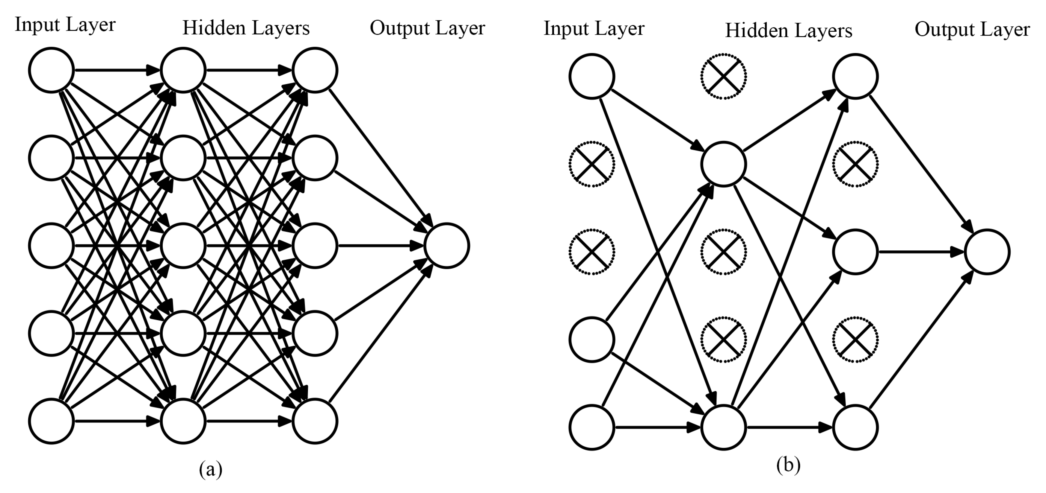
CICA is quite similar to the original ICA, with its main improvement being the assimilation policy, which controls the movement of all the colonies toward the imperialist.

Kaveh et al. [18] improved the movement method by an orthogonal vector with random variables. Talatahari et al. [12] applied chaotic functions to Kaveh et al.’s movement model to substitute these random variables. This movement is shown in Figure 3, and its equation is defined as:

$$\begin{array}{cc}\hfill {\left\{X\right\}}_{new}=& {\left\{X\right\}}_{old}+\beta \times d\times \left\{CM\right\}\otimes \left\{V_1\right\}\hfill \\ \hfill & +cm\times tan\left(\mathsf{\Theta }\right)\times d\times \left\{V_2\right\}\hfill \end{array}$$

(8)

$$\begin{array}{cc}\hfill Subjectto:& \left\{V_1\right\}·\left\{V_2\right\}=0,\hfill \\ \hfill & \left|\right|\left\{V_2\right\}\left|\right|=1\hfill \end{array}$$

where the most notations are identical to the original ICA described previously. The $cm$ represents a chaotic mapping function and $\left\{CM\right\}$ is a vector that allows the application of a different $cm$ to a different element of $\left\{V_1\right\}$. Furthermore, $\left\{V_2\right\}$ is the orthogonal unit vector of $\left\{V_1\right\}$. The sign ‘⊗’ denotes an element-by-element multiplication. Seven chaotic mapping functions and empirical parameters are shown in

Table 1. Chaotic maps.

Map	Definition	Parameters
Logistic map [19]	$x_{k+1}=a{x}_k(1-x_k)$	$a=4$
ICMIC map [20]	$x_{k+1}=sin\left(\frac{a}{x_n}\right)$	$a=0.9$
Sinusoidal map [19]	$x_{k+1}=a{x}_k^{2}sin\left(\pi x_k\right)$	$a=2.3,x_0=0.7$
Gauss map [21]	$x_{k+1}=exp(-\alpha x_k^2)+\beta$	$\alpha =4.9,\beta =-0.58$
Tent map [22]	$x_{k+1}=\mu min\{x_k,1-x_k\}$	$\mu =2$
Circle map [23]	$x_{k+1}=x_k+b-(a/2\pi )sin\left(2\pi x_k\right)mod\left(1\right)$	$a=0.5,b=0.2$
Complex squaring map [24]	$x_{k+1}=x_k^2$	$x_k=x_0^{2n}$

.

2.3. Dropout

Dropout is an efficient technique to prevent the neural network from overfitting [14]. This technique temporarily removes neurons from the network. As shown in Figure 4, the main idea is to remove the randomly chosen hidden neurons along with their connections during training.

In recent years, several works were inspired by the dropout strategy, thereby demonstrating its efficiency. Wu et al. [15] applied dropout to convolutional neural networks (CNNs) by proposing a max-pooling dropout method to probabilistically affect the output of a pooling layer. Park and Kwak [16] presented changes in the dropout probability with a uniform or normal distribution in the training iteration to make the network more robust to variations in images owing to noise. RNNdrop [17] provided a simple solution to better preserve memory when applying dropout to recurrent neural networks (RNNs). Recurrent dropout [25] applied dropout only to the hidden state of the RNN to preserve memory in a long short-term memory (LSTM). Wang et al. [26] presented a Bayesian perspective-based fast dropout technique, which regards the output of the dropout layer as sampling from a Gaussian distribution.

3. Chaotic Imperialist Competitive Algorithm with Dropout (CICA-D)

Our work was inspired by the concept of dropout. As defined in Equation (8) in CICA, all the dimensions of a colony $\left\{X\right\}$ need to be involved in the calculation. To reduce the computational complexity, we introduce dropout to the assimilation policy of CICA. The dropout strategy defines an extra hyperparameter called dropout rate, which is the probability of retaining a unit p. It is the intensity of dropout, where $p=1$ implies no dropout, and lower values of p indicate higher dropout. Our method selects a random number of dimensions from $\left\{X\right\}$ according to the dropout rate as stated by Equation (9), and subsequently applies them to Equation (8). An intuitive description is shown in Figure 5.

$$\begin{array}{c}\hfill Let\pi betheuniquepermutationof\left\{X\right\},then\\ \hfill \left\{X_{dp}\right\}=\{\pi \left(1\right),\dots ,\pi \left(N^{\prime }\right)|N^{\prime }=ceil(p·N)\}\end{array}$$

(9)

where $\left\{X\right\}$ is a colony with N dimensions. $\left\{X_{dp}\right\}$ is the dropout strategy selecting a subset of $\left\{X\right\}$ with $N^{\prime }$ dimensions according to dropout rate $p=U(0,1]$. $\pi$ selects a unique permutation from $\left\{X\right\}$. $\left\{X^{\prime }\right\}$ indicates the result of $\left\{X_{dp}\right\}$ calculated by Equation (8). $\left\{X^{\prime }\right\}$ and the retained dimensions of $\left\{X\right\}$ compose the new solution $\left\{X_{new}\right\}$.

The CICA-D is described in Algorithm 1.

Algorithm 1 CICA-D

1: Initialize and evaluate the empires with Objective function, Equations (2) and (3)  2: while convergence criterion or maximum iterations is not satisfied do  3:     Select partial dimensions of each colony with dropout rate by Equation (9)  4:     Move the colonies toward their relevant imperialist by Equation (8)  5:     if any colony in empire has a better fitness than the imperialist then  6:        Switch the positions of that colony and of the imperialist  7:     end if  8:     Compute the total power of all empires by Equations (5)–(7)  9:     Imperialistic competition(the most powerful empire catches the weakest colony from the weakest empire) 10:     if there is an empire with no colony then 11:        Eliminate the empire 12:     end if 13: end while

4. Numerical Examples

In this section, we present the numerical simulation results of CICA and CICA-D on twelve benchmark functions.

Table 2. Specifications of the benchmark problems.

Function	Definition	Interval	Optimum
Griewank	$f_1\left(X\right)=1+\frac{1}{4000}{\sum }_{i=1}^n{x}_i^2-{\prod }_{i=1}^{n}cos(\frac{x_i}{\sqrt{i}})$	[−150, 150]	0.0
Ackley	$f_2\left(X\right)=-20exp(-0.2\sqrt{\frac{1}{n}{\sum }_{i=1}^n{x}_i^2})-exp\left(\frac{1}{n}{\sum }_{i=1}^{n}cos\left(2\pi x_i\right)\right)+20+e$	[−32, 32]	0.0
Brown	$f_3\left(X\right)={\sum }_{i=1}^{n-1}{\left(x_i^2\right)}^{(x_{i+1}^2+1)}+{\left(x_{i+1}^2\right)}^{(x_i^2+1)}$	[−1, 4]	0.0
Rastrigin	$f_4\left(X\right)={\sum }_{i=1}^n(x_i^2-10cos\left(2\pi x_i\right)+10)$	[−10, 10]	0.0
Schwefel’s 2.22	$f_5\left(X\right)={\sum }_{i=1}^n|x_i|+{\prod }_{i=1}^n\left|x_i\right|$	[−100, 100]	0.0
Schwefel’s 2.23	$f_6\left(X\right)={\sum }_{i=1}^n{x}_i^{10}$	[−10, 10]	0.0
Qing	$f_7\left(X\right)={\sum }_{i=1}^n{(x^2-i)}^2$	[−500, 500]	0.0
Rosenbrock	$f_8\left(X\right)={\sum }_{i=1}^{n-1}(100{(x_i^2-x_{i+1})}^2+{(1-x_i)}^2)$	[−2.048, 2.048]	0.0
Schwefel	$f_9\left(X\right)=418.9829·n+{\sum }_{i=1}^n(-x_{i}sin\left(\sqrt{|x_i|}\right))$	[−10, 10]	0.0
Weierstrass	$f_{10}\left(X\right)={\sum }_{i=1}^n({\sum }_{k=0}^{20}({0.5}^{k}cos(2\pi ·3^k(x_i+0.5))))-n{\sum }_{k=0}^{20}({0.5}^{k}cos\left(3^k\pi \right))$	[−0.5, 0.5]	0.0
Whitley	$f_{11}\left(X\right)={\sum }_{i=1}^n{\sum }_{j=1}^n(\frac{{(100{(x_i^2-x_j)}^2+{(1-x_j)}^2)}^2}{4000}-cos(100{(x_i^2-x_j)}^2+{(1-x_j)}^2)+1)$	[−10.24, 10.24]	0.0
Zakharov	$f_{12}\left(X\right)={\sum }_{i=1}^n{x}_i^2+{\left({\sum }_{i=1}^{n}0.5i{x}_i\right)}^2+{\left({\sum }_{i=1}^{n}0.5i{x}_i\right)}^4$	[−5, 10]	0.0

details the benchmark functions, which are some well-known mathematical examples. The $f_1$–$f_6$ are symmetric, and the rest are asymmetric. We first investigate the success rates of the algorithms with seven different chaotic maps, respectively. Subsequently, we describe the detailed statistical results of the simulations. Finally, we analyze the improvement in computational complexity.

4.1. Success Rate

To discover the potential of the algorithms, we investigate the success rates on seven different chaotic maps that demonstrated efficacy in Talatahari’s work [12]. For CICA-D, we consider the different dropout rates of 0.5 and 0.1, which are extracted from the literature. In this simulation, the griewank function with N = 30 is solved 100 times by these algorithms, respectively. In addition, the maximum iteration number is set to 1000.

The success rate is defined in Equation (10) as follows.

$$S_r=100·\frac{N_{succeed}}{N_{all}}{|}_Q$$

(10)

where $N_{all}$ is the number of all trials, $N_{succeed}$ is the number of successful trials which found the solution on the Q. Q is the successful condition that is defined as:

$$|F\left(X_i\right)-F\left(X^{\ast }\right)|<=Q$$

(11)

where $F\left(X_i\right)$ is the objective function in ith iteration and $F\left(X^{\ast }\right)$ is the global optimum of the benchmark functions. The results of the success rates are presented in

Table 3. Success rate of CICA and CICA-D algorithms using different chaotic maps for Griewank function (N = 30, Q = 10⁻⁵).

	CICA	CICA-D(0.1)	CICA-D(0.2)	CICA-D(0.3)	CICA-D(0.4)	CICA-D(0.5)
Logistic map	76	63	56	38	49	52
ICMIC map	55	47	42	39	31	36
Sinusoidal map	89	83	63	72	54	67
Gauss map	23	21	19	23	14	16
Tent map	32	29	22	24	19	26
Circle map	25	22	18	8	13	10
Complex squaring map	39	32	27	25	29	27

. What stands out in the table is the dropout strategy slightly reduces the success rate, but CICA-D with a dropout rate of 0.1 can obtain a similar success rate compared to the CICA, especially with the Sinusoidal map. The results also show that the growth of the dropout rate leads to a lower success rate.

4.2. Statistical Results

To evaluate the degree of algorithm consistency, the CICA-D is used for all the benchmark functions (N = 10) described in Table 2 and subsequently compared with ICA and CICA. The CICA-D is applied with the Sinusoidal map and a dropout rate of 0.1. An empirical selection of parameter $N_{imp}$ is usually 10–20% of $N_{country}$. In our simulations, the initial $N_{imp}$ is set to 150 while $N_{country}$ is set to 1000. However, the parameters should be tuned manually for each benchmark problem to obtain the best results. The simulations are performed 30 times for each algorithm and the maximum iteration number of each trial is set to 2000.

Statistical results of

Table 4. Statistical results for Griewank function (N = 10).

	Min(best)	Mean	Max(worst)	St.Dev.
ICA	2.6990e-11	1.0341e-10	2.6780e-08	8.1404e-10
CICA	1.1707e-16	3.4777e-14	2.5794e-12	5.0708e-15
CICA-D	0	1.0767e-08	2.9765e-07	5.4310e-08

,

Table 5. Statistical results for Ackley function (N = 10).

	Min(best)	Mean	Max(worst)	St.Dev.
ICA	8.3538e-07	7.1169e-05	9.7544e-05	8.2014e-06
CICA	5.7959e-08	1.0239e-07	5.1388e-06	1.2366e-07
CICA-D	2.4248e-11	1.8701e-06	9.4602e-06	3.0191e-06

,

Table 6. Statistical results for Brown function (N = 10).

	Min(best)	Mean	Max(worst)	St.Dev.
ICA	5.3185e-03	8.2913e-02	3.4768e-01	5.9350e-02
CICA	0	3.6893e-04	7.6523e-04	2.3507e-04
CICA-D	0	1.6878e-03	3.6494e-03	1.1136e-03

,

Table 7. Statistical results for Rastrigin function (N = 10).

	Min(best)	Mean	Max(worst)	St.Dev.
ICA	0	1.6667e-06	0.00005	9.1287e-06
CICA	0	9.3427e-09	1.0685e-07	3.4296e-08
CICA-D	0	1.0604e-07	1.9899e-06	3.9926e-07

,

Table 8. Statistical results for Schwefel’s 2.22 function (N = 10).

	Min(best)	Mean	Max(worst)	St.Dev.
ICA	2.1853e-06	3.6150e-05	4.3900e-05	1.0507e-05
CICA	8.4180e-09	1.3307e-08	1.5124e-08	1.8661e-09
CICA-D	7.6125e-10	7.7876e-07	3.5125e-05	3.1734e-06

,

Table 9. Statistical results for Schwefel’s 2.23 function (N = 10).

	Min(best)	Mean	Max(worst)	St.Dev.
ICA	6.2357e-11	2.4227e-09	8.1524e-09	1.9060e-09
CICA	8.4576e-14	6.3189e-12	4.8157e-11	4.2206e-12
CICA-D	3.6451e-15	1.2597e-09	7.6530e-08	6.9023e-09

,

Table 10. Statistical results for Qing function (N = 10).

	Min(best)	Mean	Max(worst)	St.Dev.
ICA	3.7096e-04	1.2428e-03	5.8762e-02	5.2740e-03
CICA	5.2507e-08	7.8159e-08	8.3169e-07	6.9295e-08
CICA-D	1.8346e-11	6.8298e-07	7.4924e-07	1.9475e-07

,

Table 11. Statistical results for Rosenbrock function (N = 10).

	Min(best)	Mean	Max(worst)	St.Dev.
ICA	0.001296	0.201608	1.217682	0.362075
CICA	0.000182	0.024174	0.07179	0.021891
CICA-D	0.000061	0.081672	0.36303	0.101833

,

Table 12. Statistical results for Schwefel function (N = 10).

	Min(best)	Mean	Max(worst)	St.Dev.
ICA	3.2679e-06	2.9866e-05	7.2682e-05	8.4658e-06
CICA	6.2612e-09	8.1053e-09	1.5335e-08	1.2321e-09
CICA-D	5.3896e-10	6.4659e-08	4.2363e-06	3.8251e-07

,

Table 13. Statistical results for Weierstrass function (N = 10).

	Min(best)	Mean	Max(worst)	St.Dev.
ICA	2.7647e-03	3.2945e-02	6.3290e-02	1.8813e-02
CICA	0	1.5156e-05	3.1263e-05	9.8972e-06
CICA-D	0	3.9078e-04	7.9613e-04	2.5196e-04

,

Table 14. Statistical results for Whitley function (N = 10).

	Min(best)	Mean	Max(worst)	St.Dev.
ICA	5.3185e-09	3.0960e-08	3.4768e-08	7.4846e-09
CICA	6.8309e-14	9.5997e-13	7.6523e-12	6.5952e-13
CICA-D	4.2985e-15	7.3188e-11	3.6494e-10	3.3985e-11

and

Table 15. Statistical results for Zakharov function (N = 10).

	Min(best)	Mean	Max(worst)	St.Dev.
ICA	8.3546e-11	4.3202e-09	3.7554e-08	4.2478e-09
CICA	4.4263e-13	6.4897e-10	5.4924e-09	6.2908e-10
CICA-D	3.8908e-15	8.2997e-09	8.8761e-08	7.7855e-09

present the best, worst, mean, and standard deviation for the ICA, CICA, and CICA-D. Overall, the CICA-D makes a noticeable improvement in the quality of the best solution due to the enhancement of local search capability. The CICA-D obtains better results than ICA, but slightly worse than the CICA. It can be seen that the dropout strategy weakens the global exploration capability of CICA since the CICA showing better standard deviations than the CICA-D, Additionally, the CICA-D gains on global optimum straightforwardly on symmetric functions than on asymmetric functions.

4.3. Computational Complexity

The computational cost of ICA and CICA is determined by the initial number of solutions ($N_{country}$), the maximum iterations (M), and the dimensions of each solution (N). Thus, the computational complexity can be defined as $O(N_{country}\times M\times N)$. CICA-D reduces the computational complexity intuitively since it eliminates part of the dimensions of each solution using the dropout strategy. It not only reduces the number of loops but also avoids the calculation of obstacle detection on the unchanging sub-paths. Owing to the complex of real-world problems, other overhead still affects the actual computational time. In the next section, we will investigate the performance of our algorithm in solving real-world problems by applying it to path planning.

5. Application

The path planning problem is essential for autonomous underwater vehicles (AUVs) operating in a variable ocean. The most elementary form of this problem is to find an available path for AUVs, from the starting point to the destination point, while avoiding the turbulence in the ocean.

The path planning problem has been studied actively since the 1970s [27]. These algorithms can be divided into two main categories: accurate methods and heuristic methods [28,29]. Accurate methods find the globally optimal solution in a limited time and also provides the assurance of its optimality [30]. Such methods are as diverse as Roadmap Methodology [31], Cell Decomposition [32] and Artificial Potential Field [33]. A heuristic method is an approximation algorithm that explores the search space with a random process to find a near optimal solution rather than the global optimal in a limited time. Heuristic methods can be further divided into two categories: problem-specific heuristics (such as the A* algorithm) and meta-heuristics. Meta-heuristic methods, also called evolutionary algorithms, start with a set of random solutions (usually called population), and approximate the optimal solution by iteration. Several meta-heuristic algorithms are inspired by natural systems or socio-political characteristics such as genetic algorithms, artificial neural network, ant colony algorithm, particle swarm optimization(PSO), and imperialist competitive algorithm (ICA). Hocaoglu et al. [34] applied evolutionary algorithms to the global path planning problem. Jung et al. [35] proposed a neural network-based method to plan an available path in a static environment. The PSO is inspired by the social collaborative or foraging behavior of biological populations and was first proposed by Kennedy and Eberhart [36]. Huang et al. [37] successfully applied a hybrid meta-heuristic GA-PSO method to solve the global path planning problem.

Here, we apply ICA, CICA, and CICA-D to the path planning problem for AUVs operating in turbulent environments. In this study, we regard turbulent flows as obstacles that the agent should not pass through. We first define the objective function of the path planning problem. Next, we design experimental scenarios in 30 × 30 grid-based maps with irregular turbulence, and finally the experimental results are presented.

5.1. Objective Function

It is necessary to build a mathematical model to solve path planning as an optimization problem. First, we abstract the terrain into a grid-based 2D map. Figure 6 shows a sample map based on a 10 × 10 grid, and each cell of the grid has a unique index. Dark cells represent obstacles, while white cells indicate passable. The agent can move from the current cell to the available cells among its eight adjacent cells. Then we initialize a set $OBS$ with all indices of dark cells. The red line is an example of a planned path from cell 1 to cell 100 while avoiding the obstacles, and the resulting way-points are shown as the black points on the red line.

Subsequently, we define an objective function for path planning to evaluate the fitness of each solution as follows.

$$F\left(X\right)=\underset{X}{\mathrm{argmin}}(\sum _{i=1}^{N-1}D(x_i,x_{i+1}))$$

(12)

$$subjectto:X\cap OBS=\varnothing$$

where D is a function to calculate the Euclidean distance between two way-points. X is the solution with N way-points in a potential path.

$$X=\{x_1,x_2,\dots ,x_{N-1},x_N\}$$

(13)

while $x_1$ indicates the starting point, and $x_N$ indicates destination point. $OBS$ is a set of the indices of obstacles in the map. To summarize the above-mentioned equations, Equation (12) finds the solution X with the shortest path while the way-points in X do not pass through the cells in $OBS$.

5.2. Experimental Results

As shown in Figure 7, we design two 30 × 30 grid-based scenarios for the simulations.

The submarine marker in the lower-left is the starting point. The black flag marker in the upper right is the destination point. The irregular blue shapes are the turbulent areas that the agent should not pass through. To investigate the performance with different dimensions of the solution, we design that scenario 2 more complicated than scenario 1.

In the simulation, we apply the ICA, CICA, and CICA-D to the experimental scenarios, respectively. Both the CICA and CICA-D use the sinusoidal map (dropout rate is set to 0.1, 0.3, and 0.5) which performed well in Section 4. Each algorithm is executed 120 times. The performance of each algorithm is evaluated for fitness, execution time, and success rate of each. As shown in Figure 7, the solid red line indicates the optimal path generated by the proposed CICA-D method; the blue dotted line and the green dashed line indicate the optimal routes generated by ICA and CICA, respectively.

The success rate is the ratio of all near-optimal trails to the total trails. It is defined in Equation (10) with the successful condition Q defined as:

$$Q=\{F\left(X_i\right)<=F\left(X_{median}\right)|X_i\cap OBS=\varnothing \}$$

(14)

where $F\left(X_i\right)$ is the fitness of the final solution in ith trail and $F\left(X_{median}\right)$ is the median fitness of all trails. Failure trail cases are listed below.

• The optimal solution passes through the obstacles.
• The optimal solution is worse than the median of all trails.

Table 16. Performance comparison of ICA, CICA, and CICA-D with scenario 1.

		ICA	CICA	CICA-D(0.1)	CICA-D(0.3)	CICA-D(0.5)
Fitness	Min.	64.21	61.83	60.93	61.98	63.33
	Mean	66.50	63.49	64.60	66.13	67.76
	Max.	69.76	67.91	70.13	70.97	72.41
	St. Dev.	1.6335	1.1657	2.7274	2.5325	2.7108
Execution	Mean	28.67	34.91	12.87	19.81	36.03
Time (sec)	St. Dev.	14.28	18.15	7.24	8.14	14.56
Success Rate		86.67%	93.33%	87.50%	82.50%	75.83%

shows the fitness, execution time, and success rate of the original ICA, CICA, and CICA-D with scenario 1. The execution time of the CICA-D with dropout rate of 0.1 is significantly shortened, in the fact that the dropout strategy reduces the computation of each iteration by specifying only partial elements of the solution. The improvement of the best fitness of CICA-D shows that the dropout strategy enhances the local search capability; though, as a side effect, the success rate is slightly less compared to CICA due to the rising of the standard deviation of the fitness of CICA-D. Another finding from Table 16 is a more significant dropout rate affects the performance and the success rate of the proposed algorithm. Figure 8 shows the visual comparison and the convergence curve of the best solutions of ICA-, CICA-, and CICA-D-Based Path Planners with scenario 1. The CICA and CICA-D achieve similar results both visually and numerically. The rate of convergence of CICA-D is lower than the others since its elapsed iterations are increased as shown in Figure 8b.

We also applied the algorithms to a complex scenario simultaneously, as shown in Figure 9. Similar to the simulation results of scenario 1, the CICA-D with dropout of 0.1 improves the execution time and the local search capability with an insignificant loss in the success rate and the rate of convergence. The elapsed iterations of CICA-D are also increased, as shown in Figure 9b. Scenario 2 requires a more substantial dimension (N) of solutions than scenario 1 since it is more complicated. With the increase of the dimension of solutions, the execution time is raised and the success rate is reduced compared to scenario 1, as shown in

Table 17. Performance comparison of ICA, CICA and CICA-D with scenario 2.

		ICA	CICA	CICA-D(0.1)	CICA-D(0.3)	CICA-D(0.5)
Fitness	Min.	67.42	64.11	63.89	64.02	64.57
	Mean	69.68	66.18	67.57	70.28	72.62
	Max.	75.65	73.71	79.71	79.52	83.55
	St. Dev.	1.5567	1.3839	3.0785	4.0630	5.7615
Execution	Mean	52.18	57.89	17.98	46.57	69.05
Time (sec)	St. Dev.	12.41	14.59	4.79	12.48	19.24
Success Rate		80.83%	88.33%	82.50%	76.67%	70.83%

. Inappropriate dropout rate can lead to a performance degradation. This result may be explained by the fact that the loss of the increase of elapsed iterations more significant than the benefit of reducing the dimension. Based on this finding, it should be initialized with a smaller value, when tuning the parameter of the dropout rate.

In summary, the experimental results show that the proposed CICA-D with the dropout rate of 0.1 is approximately three times faster than the other algorithms. However, our approach suffers from the minor drawbacks of a slightly decreased success rate and an increased number of elapsed iterations. The elapsed iterations are increased as the dropout strategy weakens the global exploration capability while enhancing the local search potentiality. The success rate decline is due to the CICA-D having a larger standard deviation, as mentioned previously.

6. Conclusions

In this article, a novel improved chaotic imperialist competitive algorithm (CICA) integrated with a dropout strategy (CICA-D) was presented for global optimization. We introduced the dropout strategy to reduce the computational complexity of CICA. By comparing our methods with the previous ones, we investigate the success rate and the statistical properties using different benchmark functions. To demonstrate the performance and effectiveness of the proposed strategy in solving real problems, we applied the ICA, CICA, and proposed CICA-D to a path planning application, thus presenting the statistical and visual results. The simulation results showed that our proposed method with an improved dropout strategy reduced computational complexity showing three times faster execution time. In addition, the incorporation of dropout enhanced local search capability near the globally optimal solution, with only a minor drop in the success rate.

Further research could be conducted to determine the effectiveness of the proposed method on other real-world problems, such as task assignment, energy management, and training neural networks. In addition, more studies also need to be carried out to evaluate the performance of other optimization algorithms combined with the dropout strategy.

References

1. Atashpaz-Gargari, E.; Lucas, C. Imperialist competitive algorithm: An algorithm for optimization inspired by imperialistic competition. In Proceedings of the 2007 IEEE Congress on Evolutionary Computation, Singapore, 25–28 September 2007; IEEE: Piscataway, NJ, USA, 2007; pp. 4661–4667. [Google Scholar]
2. Cattani, M.; Caldas, I.L.; Souza, S.L.d.; Iarosz, K.C. Deterministic chaos theory: Basic concepts. Rev. Bras. de Ensino de Física 2017, 39. [Google Scholar] [CrossRef] [Green Version]
3. Rosso, O.; Larrondo, H.; Martin, M.; Plastino, A.; Fuentes, M. Distinguishing noise from chaos. Phys. Rev. Lett. 2007, 99, 154102. [Google Scholar] [CrossRef] [PubMed] [Green Version]
4. Chen, Y.; Li, L.; Xiao, J.; Yang, Y.; Liang, J.; Li, T. Particle swarm optimizer with crossover operation. Eng. Appl. Artif. Intell. 2018, 70, 159–169. [Google Scholar] [CrossRef]
5. Aliniya, Z.; Keyvanpour, M.R. CB-ICA: A crossover-based imperialist competitive algorithm for large-scale problems and engineering design optimization. Neural Comput. Appl. 2019, 31, 7549–7570. [Google Scholar] [CrossRef]
6. Xu, S.; Wang, Y.; Lu, P. Improved imperialist competitive algorithm with mutation operator for continuous optimization problems. Neural Comput. Appl. 2017, 28, 1667–1682. [Google Scholar] [CrossRef]
7. Ma, Z.; Yuan, X.; Han, S.; Sun, D.; Ma, Y. Improved Chaotic Particle Swarm Optimization Algorithm with More Symmetric Distribution for Numerical Function Optimization. Symmetry 2019, 11, 876. [Google Scholar] [CrossRef] [Green Version]
8. Alatas, B.; Akin, E.; Ozer, A.B. Chaos embedded particle swarm optimization algorithms. Chaos Solitons Fractals 2009, 40, 1715–1734. [Google Scholar] [CrossRef]
9. Gandomi, A.H.; Yang, X.S.; Talatahari, S.; Alavi, A.H. Firefly algorithm with chaos. Commun. Innonlinear Sci. Numer. Simul. 2013, 18, 89–98. [Google Scholar] [CrossRef]
10. Wang, G.G.; Deb, S.; Gandomi, A.H.; Zhang, Z.; Alavi, A.H. Chaotic cuckoo search. Soft Comput. 2016, 20, 3349–3362. [Google Scholar] [CrossRef]
11. Zhao, H.; Gao, W.; Deng, W.; Sun, M. Study on an Adaptive Co-Evolutionary ACO Algorithm for Complex Optimization Problems. Symmetry 2018, 10, 104. [Google Scholar] [CrossRef] [Green Version]
12. Talatahari, S.; Azar, B.F.; Sheikholeslami, R.; Gandomi, A. Imperialist competitive algorithm combined with chaos for global optimization. Commun. Nonlinear Sci. Numer. Simul. 2012, 17, 1312–1319. [Google Scholar] [CrossRef]
13. Fiori, S.; Di Filippo, R. An improved chaotic optimization algorithm applied to a DC electrical motor modeling. Entropy 2017, 19, 665. [Google Scholar] [CrossRef] [Green Version]
14. Srivastava, N.; Hinton, G.; Krizhevsky, A.; Sutskever, I.; Salakhutdinov, R. Dropout: A simple way to prevent neural networks from overfitting. J. Mach. Learn. Res. 2014, 15, 1929–1958. [Google Scholar]
15. Wu, H.; Gu, X. Towards dropout training for convolutional neural networks. Neural Netw. 2015, 71, 1–10. [Google Scholar] [CrossRef] [Green Version]
16. Park, S.; Kwak, N. Analysis on the dropout effect in convolutional neural networks. In Asian Conference on Computer Vision; Springer: Berlin/Heidelberg, Germany, 2016; pp. 189–204. [Google Scholar]
17. Moon, T.; Choi, H.; Lee, H.; Song, I. Rnndrop: A novel dropout for rnns in asr. In Proceedings of the 2015 IEEE Workshop on Automatic Speech Recognition and Understanding (ASRU), Scottsdale, AZ, USA, 13–17 December 2015; IEEE: Piscataway, NJ, USA, 2015; pp. 65–70. [Google Scholar]
18. Kaveh, A.; Talatahari, S. Optimum design of skeletal structures using imperialist competitive algorithm. Comput. Struct. 2010, 88, 1220–1229. [Google Scholar] [CrossRef]
19. May, R.M. Simple mathematical models with very complicated dynamics. In The Theory of Chaotic Attractors; Springer: Berlin/Heidelberg, Germany, 2004; pp. 85–93. [Google Scholar]
20. He, D.; He, C.; Jiang, L.G.; Zhu, H.W.; Hu, G.R. Chaotic characteristics of a one-dimensional iterative map with infinite collapses. IEEE Trans. Circuits Syst. I Fundam. Theory Appl. 2001, 48, 900–906. [Google Scholar]
21. Hilborn, R.C. Chaos and Nonlinear Dynamics: An Introduction for Scientists and Engineers; Oxford University Press on Demand: Oxford, UK, 2004. [Google Scholar]
22. Ott, E. Chaos in Dynamical Systems; Cambridge University Press: Cambridge, UK, 2002. [Google Scholar]
23. Zheng, W.M. Kneading plane of the circle map. Chaos Solitons Fractals 1994, 4, 1221–1233. [Google Scholar] [CrossRef]
24. Little, M.; Heesch, D. Chaotic root-finding for a small class of polynomials. J. Differ. Equ. Appl. 2004, 10, 949–953. [Google Scholar] [CrossRef] [Green Version]
25. Semeniuta, S.; Severyn, A.; Barth, E. Recurrent Dropout without Memory Loss. In Proceedings of the COLING 2016, the 26th International Conference on Computational Linguistics: Technical Papers, Osaka, Japan, 11–16 December 2016; pp. 1757–1766. [Google Scholar]
26. Wang, S.; Manning, C. Fast dropout training. In Proceedings of the International Conference on Machine Learning, Atlanta, GA, USA, 16–21 June 2013; pp. 118–126. [Google Scholar]
27. Choset, H.M.; Hutchinson, S.; Lynch, K.M.; Kantor, G.; Burgard, W.; Kavraki, L.E.; Thrun, S. Principles of Robot Motion: Theory, Algorithms, and Implementation; MIT Press: Cambridge, MA, USA, 2005. [Google Scholar]
28. Lamini, C.; Fathi, Y.; Benhlima, S. Collaborative Q-learning path planning for autonomous robots based on holonic multi-agent system. In Proceedings of the 2015 10th International Conference on Intelligent Systems: Theories and Applications (SITA), Rabat, Morocco, 20–21 October 2015; IEEE: Piscataway, NJ, USA, 2015; pp. 1–6. [Google Scholar]
29. Woon, S.F.; Rehbock, V. A critical review of discrete filled function methods in solving nonlinear discrete optimization problems. Appl. Math. Comput. 2010, 217, 25–41. [Google Scholar] [CrossRef] [Green Version]
30. Puchinger, J.; Raidl, G.R. Combining metaheuristics and exact algorithms in combinatorial optimization: A survey and classification. In Proceedings of the International Work-Conference on the Interplay Between Natural and Artificial Computation, Las Palmas, Canary Islands, Spain, 15–18 June 2005; Springer: Berlin/Heidelberg, Germany, 2005; pp. 41–53. [Google Scholar]
31. Šeda, M. Roadmap methods vs. cell decomposition in robot motion planning. In Proceedings of the 6th WSEAS International Conference on Signal Processing, Robotics and Automation, Corfu Island, Greece, 16–19 February 2007; World Scientific and Engineering Academy and Society (WSEAS): Athens, Greece, 2007; pp. 127–132. [Google Scholar]
32. Cai, C.; Ferrari, S. Information-driven sensor path planning by approximate cell decomposition. IEEE Trans. Syst. Man Cybern. Part B (Cybern.) 2009, 39, 672–689. [Google Scholar]
33. Rimon, E.; Koditschek, D.E. Exact robot navigation using artificial potential functions. Dep. Pap. (ESE) 1992, 323. [Google Scholar] [CrossRef] [Green Version]
34. Hocaoglu, C.; Sanderson, A.C. Planning multiple paths with evolutionary speciation. IEEE Trans. Evol. Comput. 2001, 5, 169–191. [Google Scholar] [CrossRef]
35. Jung, I.K.; Hong, K.B.; Hong, S.K.; Hong, S.C. Path planning of mobile robot using neural network. In Proceedings of the ISIE’99. IEEE International Symposium on Industrial Electronics (Cat. No. 99TH8465), Bled, Slovenia, Slovenia, 12–16 July 1999; IEEE: Piscataway, NJ, USA, 1999; Volume 3, pp. 979–983. [Google Scholar]
36. Kennedy, J. Particle swarm optimization. In Encyclopedia of Machine Learning; Springer: Berlin/Heidelberg, Germany, 2010; pp. 760–766. [Google Scholar]
37. Huang, H.C.; Tsai, C.C. Global path planning for autonomous robot navigation using hybrid metaheuristic GA-PSO algorithm. In Proceedings of the SICE Annual Conference, Tokyo, Japan, 13–18 September 2011; IEEE: Piscataway, NJ, USA, 2011; pp. 1338–1343. [Google Scholar]
Figure 1. Flowchart of the original ICA.
Symmetry 12 00635 g001
Figure 2. Movement of colony to its new location in ICA.
Symmetry 12 00635 g002
Figure 3. Movement of colony to its new location in CICA.
Symmetry 12 00635 g003
Figure 4. Dropout Strategy. (a) A standard neural network. (b) Applying dropout to the neural network on the left by dropping the crossed units.
Symmetry 12 00635 g004
Figure 5. Incorporation of Dropout into the assimilation policy of CICA, the gray cell of { X } is dropped.
Symmetry 12 00635 g005
Figure 6. A grid-based map example.
Symmetry 12 00635 g006
Figure 7. Scenarios for simulation. Submarine marker: the starting position. Flag marker: the destination. Blue irregular shape: the turbulence. Solid red line: the optimal path by CICA-D; blue dotted line: the optimal path by ICA; green dashed line: the optimal path by CICA.
Symmetry 12 00635 g007
Figure 8. Comparison of ICA-, CICA-, and CICA-D-Based Path Planners with Scenario 1.
Symmetry 12 00635 g008
Figure 9. Comparison of ICA-, CICA-, and CICA-D-Based Path Planners with Scenario 2.
Symmetry 12 00635 g009