Abstract
Linguistic interval-valued intuitionistic fuzzy sets, as an extension of interval-valued intuitionistic fuzzy sets, have strong practical value in the management of complex uncertainty system with qualitative evaluation information. This study focuses on the development of several linguistic interval-valued intuitionistic fuzzy Hamacher (LIVIFH) aggregation operators based on the extended Hamacher t-norm and s-norm. First, the extended Hamacher t-norm and s-norm, which are applicable to linguistic information environment, are applied to define the linguistic interval-valued intuitionistic fuzzy Hamacher operational laws. Second, based on the proposed operational laws, this study defines the linguistic interval-valued intuitionistic fuzzy Hamacher weighted average (LIVIFHWA) operator and the linguistic interval-valued intuitionistic fuzzy Hamacher weighted geometric (LIVIFHWG) operator, and then investigates their properties. Furthermore, the degeneracy and monotonicity of the proposed operators with respect to the adjustable parameter are explored. Finally, a multiple attribute group decision-making (MAGDM) approach is developed based on the proposed LIVIFH aggregation operators, and then this approach is applied to a supplier selection problem. Parameter analysis indicates that the adjustable parameter in the proposed LIVIFH aggregation operators could reflect the attitudes of decision makers. The LIVIFHWA operator would be more appropriate to optimistic decision makers, and the LIVIFHWG operator to pessimistic decision makers. In addition, as the adjustable parameter increasing, both attitudes tend to be neutral. The proposed method is also compared with two other approaches to show its feasibility and efficiency.
1. Introduction
Linguistic multi-attribute group decision-making (LMAGDM) is an important branch in decision theory. When making qualitative evaluations for alternative-to-attribute objects in the decision-making process, experts get used to use linguistic variables [1], such as “Reject”, “Major revision”, “Minor revision”, and “Accept”, rather than numerical scales. Ordered qualitative scales generated by linguistic variable are common in social sciences, engineering, computer sciences, and other fields. Along with the development of fuzzy information processing technology, many extensions based on the concept of linguistic variable have been introduced in recent years, such as 2-tuple fuzzy linguistic representation model [2], virtual linguistic model [3], proportional 2-tuple linguistic variable [4], etc. These extended concepts and models support the construction of normative description, operation and aggregation of linguistic evaluation information, and improve the efficiency of solving LMAGDM problems. Furthermore, as the LMAGDM problems are getting complicated, in order to facilitate the integration of linguistic evaluation information provided by group experts, scholars have extended statistical methods such as probability theory, possibility theory, and proportional concepts to linguistic variables based on hesitant fuzzy sets [5], and proposed various corresponding distribution linguistic term sets (DLTSs) [6,7,8,9,10,11]. Decision-makers can apply these DLTSs based on the characteristics of MAGDM problems and linguistic evaluation information from experts. The DLTSs show its wide applicability in the fields of medical treatment [12,13], product evaluation [14,15], engineering construction [16], and public emergency [17,18,19].
It is worth noting that the above-mentioned DLTSs focus on the qualitative representation of membership degree, and do not pay attention to the non-membership degree that can feedback experts’ negation. In order to comprehensively consider the advantages of membership and non-membership in characterizing experts’ psychological characteristics, scholars extended the concept of intuitionistic fuzzy sets (IFSs) [20] to linguistic information environment and proposed linguistic intuitionistic fuzzy sets (LIFSs) [21,22]. LIFSs could qualitatively represent membership or non-membership through linguistic variables. When dealing with LMAGDM problems, linguistic aggregation operator is usually the key technique to fuse the evaluation information of multiple experts. In order to deal with the LMAGDM problem with attribute association, based on the Power average (PA), Bonferroni mean (BM) and Heronian mean (HM), the linguistic intuitionistic PA, BM and HM operators [23,24,25,26] are developed. Some aggregation operators that can capture and reflect and interrelationships among aggregated arguments are intensively studied, which include the linguistic intuitionistic Hamy and Shapley fuzzy operator [27,28]. They enrich the linguistic intuitionistic fuzzy set theory and its decision-making method. However, in some complex LMAGDM problems, it is difficult for experts to provide accurate linguistic terms, instead, it is not uncommon to represent preference through interval-valued linguistic numbers [29]. Therefore, some scholars [30,31] put forward the concept of linguistic interval-valued intuitionistic fuzzy sets (LIVIFSs), so that experts can use interval-valued linguistic terms to express the membership degree and non-membership degree of alternatives under evaluation attributes. Some algebraic operational laws [30,31] are defined to construct the interval-valued linguistic intuitionistic fuzzy aggregation operators. A rank method is developed to distinguish between different interval-valued linguistic intuitionistic fuzzy numbers (LIVIFNs) by proposing the score and accuracy functions [30,31].
In developing various linguistic term sets such as hesitant fuzzy linguistic term sets (HFLTSs), LIFSs, and DLTSs, the basic operations play a critical role, and LIVIFSs is no exception. However, few studies have been conducted with regard to the operations for LIVIFSs [30,31], especially for the generalized operations. In fact, based on the Hamacher t-norm and s-norm [32], several generalized operations on various types of extended fuzzy sets have been developed, such as intuitionistic fuzzy Hamacher operations [33], hesitant fuzzy Hamacher operations [34], and Pythagorean fuzzy Hamacher operations [35]. Two main characteristics of Hamacher t-norm and s-norm are that: (i) decision-makers (DMs) can obtain various types of t-norm and s-norm by selecting different parameter values. In the cases of and , for example, the Hamacher t-norm(s-norm) will reduce to the Algebraic t-norm(s-norm) and Einstein t-norm(s-norm), respectively, and (ii) the Hamacher t-norm and s-norm would decrease and increase respectively with the increasing of parameter . When solving group decision-making problems, these properties will provide a new perspective for the analysis of expert behavior. What needs to be mentioned is that, based on the traditional t-norm and s-norm, literature [36] proposed extended t-norm and s-norm that are suitable for LMAGDM environment, and constructed a serial of generalized operations and aggregation operators of linguistic term sets.
Inspired by their research, based on the Hamacher operational laws, to the current study develops the linguistic interval-valued intuitionistic fuzzy Hamacher weighted average (LIVIFHWA) and interval-valued intuitionistic fuzzy Hamacher weighted geometric (LIVIFHWG) operators, which will be used to fuse the evaluation information of multiple experts. Then, the relationships between the proposed linguistic interval-valued intuitionistic fuzzy Hamacher (LIVIFH) aggregation operators and their corresponding adjustable parameters will be explored, focused on the degeneracy and monotonicity properties. Finally, based on the proposed LIVIFH aggregation operators, a MAGDM approach is developed to deal with the problems with LIVIFNs, and the practical meaning of the adjustable parameters is illustrated accordingly through a numerical example.
The rest of the paper is structured as follows. Some preliminaries of LIVIFSs and extended Hamacher t-norm(s-norm) are provided in Section 2. In Section 3, the linguistic interval-valued intuitionistic fuzzy Hamacher operations and operator are proposed, and their special cases and desire properties are explored. Furthermore, in Section 4, this study proposes a LIVIF MAGDM approach for solving the LMAGDM problems, and applies this method to select a platform supplier for a large corporation. Finally, Section 5 concludes this paper.
2. Preliminaries
This section introduces primarily the definitions of LIVIFSs as well as their operational laws. Some concepts of the extended Hamacher t-norm and s-norm are also introduced.
Definition 1.
[1] Letbe a finite and totally ordered linguistic term set, andis a positive integer andis the possible value of linguistic variable. We callas a discrete linguistic set ifsatisfies: (i) if, then; (ii) there exists negation function, so that .
For ease of calculation, literature [37] extended the discrete linguistic set into continuous linguistic set , and also satisfied the aforementioned conditions.
Generalization of interval-valued intuitionistic fuzzy set and linguistic term set leads to the concept of a linguistic interval-valued intuitionistic fuzzy set, which provides the more freedom to the decision-makers [31].
Definition 2.
[30,31] Letbe a fixed set and be a continuous linguistic set. Then a linguistic interval-valued intuitionistic fuzzy set associated with can be written as
where and are the membership degree and non-membership degree, respectively, and . is the hesitant degree of .
For convenience, we call as linguistic interval-valued intuitionistic fuzzy number (LIVIFN) and simply express it as , where and , and ,.
Definition 3.
[31] Let be two LIVIFNs, then
- (1)
- if, then ;
- (2)
- if, then ;
- (3)
- the negation ofis defined as .
To compare the LIVIFNs, the score function and accuracy function are defined as follows.
Definition 4.
[31] Letbe a LIVIFN, then the score function and accuracy function ofare defined asand , respectively.
Letbe two LIVIFNs, then the rank method based on score function and accuracy function are defined as follows:
- (1)
- if, then ;
- (2)
- if , , then .
Next, we introduce the existing operational laws and weighted aggregation operators for LIVIFNs.
Definition 5.
[30,31] Letbe two LIVIFNs, and parameter, then some operational laws of1are defined as follows:
- (1)
- ;
- (2)
- ;
- (3)
- ;
- (4)
- .
Definition 6.
[31] Let,, be a collection of LIVIFNs, then
- (1)
- the linguistic interval-valued intuitionistic fuzzy weighted average (LIVIFWA) operator is a mapping given by
- (2)
- the linguistic interval-valued intuitionistic fuzzy weighted geometric (LIVIFWG) operator is a mappinggiven bywhereis the weight vector, and .
Extended Hamacher T-Norm and S-Norm
Next, we require some related concepts of Hamacher t-norm and s-norm, which are the core theoretical tools for constructing linguistic interval-valued intuitionistic fuzzy Hamahcer laws and aggregation operators. Then, we analyse the relationship between Hamacher t-norm(s-norm) and extended Hamacher t-norm(s-norm) based on the negative function.
Definition 7.
A functionis called an extended negation function if it satisfies the following conditions: (1)is continuous; (2); (3) if, then; (4) .
Definition 8.
Given an extended negation function ,
- (1)
- ifsatisfies: (1),; (2),,, thenis called an extended aggregation function.
- (2)
- ifsatisfies, thenandare dual aggregation function with.
Definition 9.
A mappingis called an extended triangular norm (t-norm) if it satisfies the following conditions:
- (1)
- Commutativity:;
- (2)
- Associativity:;
- (3)
- Monotonicity:;
- (4)
- Neutral element:.
Definition 10.
A mappingis called an extended t-conorm (s-norm) if it satisfies the following conditions:
- (1)
- Commutativity:;
- (2)
- Associativity:;
- (3)
- Monotonicity:;
- (4)
- Neutral element:.
Definition 11.
Given an extended t-norm and s-normand, thenandare dual with respect to functionif and only if
Remark 1.
When, some degenerate properties of above functions is provided: (1) extended negative functionreduce to the traditional negative function [38]; (2) extended aggregation functionreduce to the aggregation function in unit interval [38]; (3) extended t-norm and s-norm reduce to the traditional t-norm and s-norm [38].
On the basis of Hamacher t-norm and s-norm, the research [32] proposed the extended Hamacher t-norm and s-norm.
Definition 12.
A mappingis called an extended Hamacher t-norm if it satisfies:
where the parameter.is the generator ofand.is the pseudo inverse function of,and.
Definition 13.
A mappingis called an extended Hamacher s-norm if it satisfies:
where the parameter.is the generator of, and
whereis negation function and.
Theorem 1.
Letandbe a pair of dual extended Hamacher t-norm and s-norm, then
- (1)
- ;
- (2)
According to Theorem 1, and are dual with respect to .
3. Linguistic Interval-Valued Intuitionistic Fuzzy Hamacher Aggregation Operators
3.1. Linguistic Interval-Valued Intuitionistic Fuzzy Hamacher Operational Laws
In the theoretical study of fuzzy sets, t-norm and s-norm are generally used to construct operational laws, while laws are further used to construct aggregation operators, which are progressive layer by layer. Next, we will use the extended Hamacher t-norm and s-norm to construct the Hamacher operational laws.
Definition 14.
Letbe two LIVIFNs,, then linguistic interval-valued intuitionistic fuzzy Hamacher operational laws is defined as following:
- (1)
- ;
- (2)
- ;
- (3)
- ;
- (4)
- .
whereandare generators ofand. Functionandsatisfy:
Theorem 2.
The operator laws in definition 14 is closed.
Proof.
Need to prove that and are LIVIFNs. Since are LIVIFNs, then .
(1) To prove is closed is equivalent to prove that . Since is monotonicity, and , then
,
Therefore,
.
Thus, is also a LIVIFN.
(2) To prove is closed is equivalent to prove that . Since is monotonicity, and , then
Therefore,
,
Thus, is also a LIVIFN.
Similarly, and is also closed. □
Moreover, some relations of the operational laws can be summarized as follows:
Theorem 3.
Letbe two LIVIFNs, and, then
- (1)
- ;
- (2)
- ;
- (3)
- ;
- (4)
- ;
- (5)
- ;
- (6)
- .
3.2. Linguistic Interval-Valued Intuitionistic Fuzzy Hamacher Aggregation Operators
Aggregation operators are one of the most powerful tools in the fuzzy multi-attribute decision-making (MADM) problems, in which fusing fuzzy information from various sources is required. In this subsection, the proposed Hamacher operational laws are used to construct two LIVIFH operators, namely, the linguistic interval-valued intuitionistic fuzzy Hamacher weighted average (LIVIFHWA) operator and the linguistic interval-valued intuitionistic fuzzy Hamacher weighted geometric (LIVIFHWG) operator.
3.2.1. LIVIFHWA Operator and LIVIFHWG Operator
Definition 15.
Letbe a collection of LIVIFNs,is the weight vector, and. Then the linguistic interval-valued intuitionistic fuzzy Hamacher weighted average (LIVIFHWA) operator is mapping, which satisfies
Theorem 4.
Letbe a collection of LIVIFNs, then
Proof.
This is easy to prove according to induction. □
Definition 16.
Letbe a collection of LIVIFNs,is the weight vector, and. Then the linguistic interval-valued intuitionistic fuzzy Hamacher weighted geometric (LIVIFHWG) operator is mapping, which satisfies
Theorem 5.
Letbe a collection of LIVIFNs, then
3.2.2. Some Properties of Two LIVIFH Operators
Before discussing the concrete forms and related properties of the proposed LIVIFH operators, we first construct a pair of dual Hamacher functions.
Definition 17.
Letandbe the generator of extended Hamacher t-normand s-normrespectively, then
(1) A Hamacher aggregation functionis defined as
(2) A dual Hamacher aggregation functionis defined as
Now, a desirable property of above dual Hamacher functions is investigated in detail.
Theorem 6.
Given two aggregation operators defined in Definition 17, then
(1);
(2).
Proof.
Only (1) is proved here, it is similar for (2). Since , ,
Thus, . □
The following theorem reveal that the closed relations between the above dual aggregation functions and the LIVIFH operators.
Corollary 1.
Letbe a collection of LIVIFNs, then
(1);
(2).
Besides, some other basic properties of the LIVIFH operators are also studied.
Theorem 7.
Letbe a collection of LIVIFNs, then
(1) The LIVIFHWA operator and LIVIFHWG operator are closed.
(2) If,, then
(3) Letbe a collection of LIVIFNs, and, then
Proof.
As is a collection of LIVIFNs, then
(1) According to Inference 1, operator LIVIFHWA is closed is equivalent to . Then according to the monotonicity of and Theorem 6(2), we have
Thus, the LIVIFHWA operator is closed. Similarly, the LIVIFHWG operator is also closed.
(2) This is easy to prove according to idempotency.
(3) According the monotonicity of aggregation function and ,
□
Case 1. If hold for each , i.e., , then
Case 2. If there exists that does not satisfy , assume that , then .
According score function,
therefore,
Similarly, we can prove that
Theorem 8.
Letbe a collection of LIVIFNs, then
(1);
(2).
Proof.
According Inference 1,
Similarly,
□
3.3. Relationship between Operator and Parameter
In this subsection, we will discuss the relationship between two kinds of operators and their related parameters, including the degeneracy and the monotonicity of operators with regard to parameters.
3.3.1. Limiting Cases of LIVIFH Operators
Before moving forward to the investigation of degeneracy of the LIVIFHWA and LIVIFHWG operators, we study the limiting cases of the dual Hamacher functions with adjustable parameters.
Lemma 1.
Letandbe functions defined in Definition 17, then
- (1)
- ;
- (2)
- ;
- (3)
- ;
- (4)
- ;
- (5)
- ;
- (6)
- ;
- (7)
- ;
- (8)
- .
Proof.
We only proved (1), (2), (7) and (8) here.
- (1)
- According to Definition 17 and L’Hospital’s rule,
- (2)
- According to Theorem 6,
- (3)
- According to Definition 17,
- (4)
- According to Definition 17,□
Remark 2.
In the following, the limit function of,, will be denoted as, the limit function of,, will be denoted as,.
Based on the above analysis and the internal relationship between dual Hamacher functions and operators, the relationship between operators and parameters are analyzed below.
Theorem 9.
Letbe a collection of LIVIFNs, then
- (1)
- When, the LIVIFHWA operator degenerates into the Harmonic weighted average (LIVIFHarWA) operator:
- (2)
- When, the LIVIFHWG operator degenerates into the Harmonic weighted geometric (LIVIFHarWG) operator:
- (3)
- When, the LIVIFHWA operator degenerates into the Algebraic weighted average (LIVIFAWA) operator:
- (4)
- When, the LIVIFHWG operator degenerates into the Algebraic weighted geometric (LIVIFAWG) operator:
- (5)
- When, the LIVIFHWA operator degenerates into the Einstein weighted average (LIVIFEWA) operator:
- (6)
- When, the LIVIFHWG operator degenerates into the Einstein weighted geometric (LIVIFEWG) operator:
- (7)
- When, the LIVIFHWA operator degenerates into the Symmetric weighted average (LIVIFSWA) operator:
- (8)
- When, the LIVIFHWG operator degenerates into the Symmetric weighted geometric (LIVIFSWG) operator:
3.3.2. Monotonicity of Operators with Respect to Their Parameters
The degeneracy of the operator with respect to parameters is mainly based on the perspective of the discrete value of the parameter. Below we analyze the relationship between the operator and the parameter from the perspective of the continuous value of the parameter. First, the monotonicity of dual Hamacher functions with respect to their parameters are discussed.
Lemma 2.
decreases with increasing parameter, whileincreases with increasing parameter.
Proof.
(1) Since , then the derivation of regarding would be
Thus, , increases with increasing parameter .
(2) According to Theorem 6,
□
According to (1), increases with increasing parameter , then decreases with increasing parameter .
Next, the monotonicity of operators with respect to their parameters are analyzed below.
Theorem 10.
Letbe a collection of LIVIFNs, then,
- (1)
- The LIVIFHWA operator decreases with increasing parameter;
- (2)
- The LIVIFHWG operator increases with increasing parameter.
Proof.
According to Theorem 6 and the definition of score function,
Then according to Lemma 2,
is strictly monotone decreasing regarding .
is strictly monotone increasing regarding . Therefore, the LIVIFHWA operator decreases with increasing parameter , and the LIVIFHWG operator increases with increasing parameter . □
4. Multiple Attributes Decision-Making Approach Based on the LIVIFH Operators and Its Application
In this section, the proposed linguistic interval-valued intuitionistic fuzzy Hamacher operators were applied for solving the supplier selection problem.
4.1. Supplier Selection Problem
The supplier selection problem is a typical MADM problem. Decision makers need to evaluate suppliers based on a set of evaluation indicators, and then select the best supplier for cooperation. With the rapid development of economy and the increasing complexity of society, the knowledge and experience from various fields become essential in this decision-making process. To improve the reliability and rationality of the decision, a comprehensive evaluation of suppliers through an expert group is necessary. Therefore, the supplier selection problem is gradually transformed into a MAGDM problem. The supplier selection MAGDM problem generally consists of four parts: supplier alternatives, group of experts, evaluation attributes, and decision-making information matrixes. For convenience, the symbols of some sets and variables associated with the supplier selection problem will be expressed uniformly as follows.
- (1)
- Supplier alternatives: Let be the set of supplier alternatives, where denotes the th supplier alternative, . The best supplier will be selected from the set of alternatives.
- (2)
- Evaluation attributes: is the set of attributes for the supplier alternatives, where is the th attribute, .
- (3)
- Group of experts: Let be the experts from different research areas, where is the th expert,. is the weight vector of experts, where is the weight of the expert , and satisfies and for . The decision maker aims to coordinate the insights of different experts and select the best one out of supplier alternatives measured on attributes.
- (4)
- Decision-making information matrixes: The experts are requested to express their preferences by using LIVIFNs generated by a discrete linguistic set , which described in Definition 1. For an alternative with respect to an attribute , an expert provides his/her assessments by using LIVIFNs . By collecting each attribute’s evaluation information from expert , the decision-making information matrix is obtained. is continuous virtual linguistic term set with respect to , and ,, , , .
4.2. Decision-Making Method for Solving Supplier Selection Problem
Based on the proposed aggregation operators, the LIVIF MAGDM method is constructed as the following:
Step 1. Obtain decision-making matrix by collecting assessment information from experts.
Step 2. Aggregate the individual evaluation matrix into a collective evaluation matrix by using the LIVIFHWA operator or the LIVIFHWG operator.
Step 3. Aggregate the attribute values with respect to alternative in matrix by using the LIVIFHWA operator or the LIVIFHWG operator, and obtain the comprehensive evaluation values :
Step 4. Rank the comprehensive evaluation values based on the score function
Step 5. According to the rank of , obtain the rank of alternatives:
4.3. Case Study
In this section, an example was provided to illustrate how the proposed LIVIF MAGDM method was working in practice. Then a parametric analysis was performed to verify the rationality of the relevant Theorems, and to show that the proposed operators had the ability to reflect the decision attitude characteristics. Finally, the proposed LIVIF MAGDM method was compared with the existing two approaches that could deal with the MADM problem involving LIVIFSs.
4.3.1. Illustrative Example
Assume that a large corporation needs to build a data platform. There are four alternative platform suppliers , and the large corporation consults three experts to select the most suitable one, and assume the weight vector for evaluation experts is . The four platform suppliers are assessed based on four evaluation attributes [39]: Quality , “Rationality of Price , After Sales Performance , Delivery Time Performance , with the corresponding weight vector being . Based on the given linguistic term set
experts use the LIVIFNs to provide their evaluation information matrix , where is an LIVIFN. The proposed MAGDM method in Section 4.2 is applied to fuse different experts’ opinions to get the final decision.
Step 1. Collect the evaluation information from expert group, the decision matrix for experts are shown in Table 1.

Table 1.
Evaluation matrixes of experts.
Step 2. Aggregate individual evaluation matrix into a comprehensive matrix by using the LIVIFHWA operator (set ).
and where
Step 3. Aggregate the line element of alternative in matrix through the LIVIFHWA operator,
where
and then obtain :
Step 4. Calculate the score function value for each collective evaluation value
Therefore, according the score function value.
Step 5. According to the comprehensive evaluation rank, obtain the alternatives rank , and the optimal alternative .
4.3.2. Parameter Analysis
In the multi-attribute decision-making process, compared with traditional quantitative representations, the qualitative linguistic term representations can sometimes better reflect the experts’ preferences on the alternatives. Therefore, based on the example provided, we illustrated this property through parameter analysis.
To investigate to what extent the change of parameter can influence the MAGDM results, we calculated and compared different results as the parameter varying within a given range (). Use the LIVIFHWA operator and the LIVIFHWG operator to obtain the score values of four alternatives, as shown in Figure 1 and Figure 2, respectively. For convenience, denote the comprehensive evaluation value based on the LIVIFHWA operator as , and denote the comprehensive evaluation value based on the LIVIFHWG operator as .
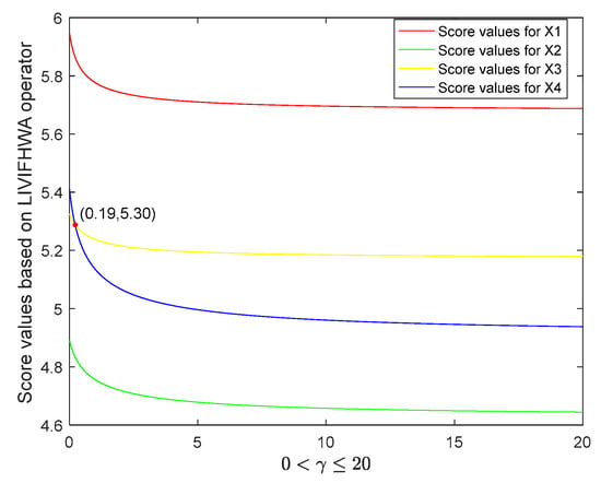
Figure 1.
Score values of alternatives based on the linguistic interval-valued intuitionistic fuzzy Hamacher weighted average (LIVIFHWA) operator.
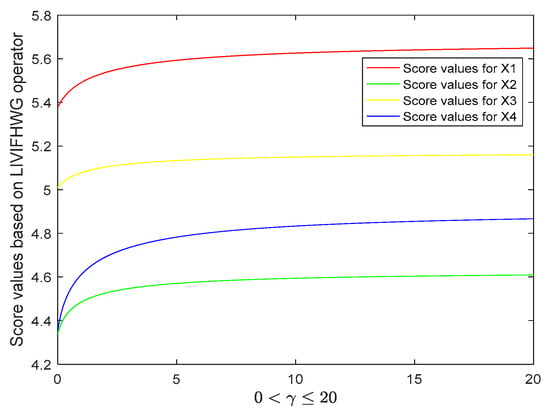
Figure 2.
Score values of alternatives based on the linguistic interval-valued intuitionistic fuzzy Hamacher weighted geometric (LIVIFHWG) operator.
Case 1. Figure 1 shows the score values of four alternatives based on the LIVIFHWA operator.
- (1)
- decreased with increasing parameter. This is consistent with the Theorem 10 (1);
- (2)
- When , the rank of alternatives was ; when , the rank of alternatives was , which means the rank of alternatives and switched. This is because the decreasing in score value of was relatively smaller compared with that of . Alternative was always the optimal alternative.
Case 2. Figure 2 shows the score values of alternatives based on LIVIFHWG operator.
- (1)
- increased with increasing parameter . This is consistent with the Theorem 10 (2);
- (2)
- The rank of alternative was always .
Case 3. Furthermore, we also explored the relationships between the two general operators (LIVIFHWA/LIVIFHWG) and the other three special aggregation operators (LIVIFHarWA, LIVIFHarWG, and LIVIFSWA), their score values are depicted in Figure 3 and Figure 4 when parameter .
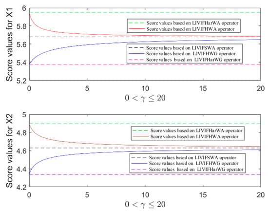
Figure 3.
Score values of alternatives X1/X2 based on five different operators.
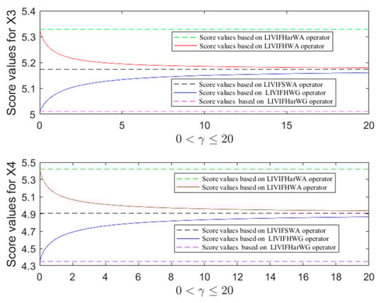
Figure 4.
Score values of alternatives X3/X4 based on five different operators.
- (1)
- The difference between score values of LIVIFHWA operator and LIVIFHarWA operator increased with increasing parameter, while the difference between score values of LIVIFHWA operator and the LIVIFSWA operator decreased.
- (2)
- The difference between score values of LIVIFHWG operator and LIVIFHarWG operator increased with increasing parameter, while the difference between score values of LIVIFHWG operator and LIVIFSWA operator decreased.To summarize, the relationships between the score values of these five operators were:
Based on the above analysis, the aggregation value of the LIVIFHWA operator was always greater than the value of the LIVIFHWG operator. As the increasing of parameter , their difference became smaller and reduced towards 0 when the parameter tended to infinity. Therefore, the LIVIFHWA operator would be more appropriate to optimistic decision makers. The bigger of the parameter represents the lower of the optimistic level. When the parameter approaches infinity, the decision maker’s attitude tended to be neutral. In contrast, the LIVIFHWG operator would be more appropriate to pessimistic decision makers. The bigger of the parameter represents the lower of the pessimistic level. When the parameter approaches infinity, the decision maker’s attitude tended to be neutral.
4.3.3. Comparative Analysis
For the MADM problem involving LIVIFSs, there are only two existing approaches available [30,31]. Therefore, in this section we made a straightforward comparison between our result and the results based on these two approaches.
(1) Comparison with the decision-making method in reference [30].
Liu and Qin [30] proposed the weighted interval-valued linguistic intuitionistic fuzzy Maclaurin symmetric mean (WIVLIFMSM) operator, and applied the WIVLIFMSM operator to solve the MADM problems with LIVIFSs.
First, based on the case study in Section 4.3.1, the operators in this paper were compared with the WIVLIFMSM operator in [30]. Since the WIVLIFMSM operator is only applicable for MADM, not for MAGDM, our approach was used to obtain the comprehensive matrix (step 1 and step 2). Then, assuming that its parameter , we applied the WIVLIFMSM operator to solve the comprehensive matrix . For more details regarding this operator and method, we encourage readers to consult [30].
Step 1–2. Same as in Section 4.3.1.
Step 3. Use the WIVLIFMSM operator to produce the comprehensive evaluation values :
Step 4. Calculate the score function value of collective evaluation value
Therefore, according the score function value.
Step 5. According to the comprehensive evaluation rank, obtain the alternatives rank , and the optimal alternative .
The decision results by using the WIVLIFMSM operator was the same as that of the LIVIFHWA operator in this paper under the limit of .
Second, based on the inner structure of operators, a comparative analysis was carried out between the WIVLIFMSM operator and the LIVIFHWA operator in this paper.
According to the Theorem 6 in [30], the WIVLIFMSM operator was decreasing when the parameter increased, . While from theorem 10(1) in Section 3.3.2 of the current study, the LIVIFHWA operator also decreased with increasing parameter , and the parameter was continuous. Moreover, regarding the degeneracy, some special cases of the WIVLIFMSM operator was analyzed with respected to the parameter in [30]. For example, when , the WIVLIFMSM operator degenerated into the LIVIFAWA operator [30]. Interestingly, according to theorem 9(3), the LIVIFHWA operator in this paper could also degenerate into the LIVIFAWA operator when .
The above comparative analysis indicates that the operators proposed in the current study had the same properties as those in [30]. In addition, the decision-making method in this paper could deal with MAGDM problems.
(2) Comparison with decision-making method in reference [31].
In [31], the LIVAIFWA operator and LIVAIFWG operator are developed to solve the MAGDM problems with LIVIFSs. In fact, according to Theorem 9(3) and (5), when , the LIVIFHWA operator and the LIVIFHWA operator in this paper reduced to the LIVAIFWA operator and LIVAIFWG operator in [31], respectively. Thus, when applying the LIVAIFWA operator and LIVAIFWG operator to solve the MAGDM problem in the Section 4.3, we could obtain the same decision results as the LIVIFHWA operator () and the LIVIFHWG operator : .
In comparison to the WIVLIFMSM and the LIVAIFWA/LIVAIFWG operators, the proposed LIVIFH aggregation operators could be concluded with the following merits.
- (1)
- The adjustable parameter could reflect the DM’s attitude.The parameter analysis has manifested that the LIVIFH aggregation operators were capable of reflecting the DM’s preferences by determining the appropriate values of the adjustable parameter .
- (2)
- The expansion of the domain for evaluation.The WIVLIFMSM operator could deal with MADM problems with LIVIF inputs, but not MAGDM problems. While the LIVAIFWA/LIVAIFWG operators are capable of dealing with MAGDM problems with LIVIF inputs, but they were merely degenerate cases of the proposed LIVIFHWA and LIVIFHWG operators when the adjustable parameter .
5. Conclusions
Linguistic interval-valued intuitionistic fuzzy set is proposed in [30,31] by combining the concepts of linguistic variable and the interval-valued intuitionistic fuzzy set. Its prominent properties are that that (i) represent the preference like the linguistic variable does and (ii) consider both membership and non-membership information. The Hamacher t-norm and s-norm are popular in defining operations and aggregation operators of various fuzzy sets because of their advantages on parameter degeneracy and monotonicity. With these considerations, the extended Hamacher t-norm and s-norm were used to the LIVIF environment in this paper.
In this study, we applied the extended Hamacher t-norm and s-norm to define the linguistic interval-valued intuitionistic fuzzy Hamacher operations. We revealed that the operations for LIVIFNs in reference [31] were a special case of generalized operation in this paper. Some basic properties of this generalized operations, such as its closeness and exchangeability, were discussed. Then, we constructed the LIVIFHWA and LIVIFHWG operators on the basis of the developed Hamacher operations, and investigated their instrumental properties. Several limiting cases of the LIVIFHWA and LIVIFHWG operators have been explored with regard to the introduced adjustable parameter. Based on the LIVIFHWA (or LIVIFHWAG) operator, we developed a new decision-making technique for the classical LMAGDM problem, and verified its applicability and feasibility through an example of supplier selection problem. Furthermore, the parameter analysis illustrated the adjustable parameter’s capability to reflect the DM’s attitudes, and the comparative analysis showed the superiority of the proposed LIVIFHWA and LIVIFHWG operators over the previous techniques.
Author Contributions
Conceptualization, W.-B.Z.; methodology, W.-B.Z.; software, W.-B.Z.; validation, W.-B.Z.; formal analysis, W.-B.Z.; data curation, W.-B.Z.; writing—original draft preparation, W.-B.Z.; writing—review and editing, W.-B.Z. and B.S. and S.-H.Z.; visualization, W.-B.Z.; supervision, W.-B.Z. and S.-H.Z.; funding acquisition, B.S. All authors have read and agreed to the published version of the manuscript.
Funding
This research was funded by National Natural Science Foundation of China, NO. 71173177; Science and technology service project of transportation supervision department of national railway administration; Southwest Jiaotong University “Double-First Class” Construction Project NO.JDSYLYB2018029.
Conflicts of Interest
The authors declare no conflict of interest.
References
- Zadeh, L. The concept of a linguistic variable and its application to approximate reasoning—I. Inf. Sci. 1975, 8, 199–249. [Google Scholar] [CrossRef]
- Martinez, L.; Herrera, F. A 2-tuple fuzzy linguistic representation model for computing with words. IEEE Trans. Fuzzy Syst. 2000, 8, 746–752. [Google Scholar] [CrossRef]
- Xu, Z. Deviation measures of linguistic preference relations in group decision making. Omega 2005, 33, 249–254. [Google Scholar] [CrossRef]
- Wang, J.-H.; Hao, J. A new version of 2-tuple fuzzy linguistic representation model for computing with words. IEEE Trans. Fuzzy Syst. 2006, 14, 435–445. [Google Scholar] [CrossRef]
- Torra, V. Hesitant fuzzy sets. Int. J. Intell. Syst. 2010, 25, 529–539. [Google Scholar] [CrossRef]
- Rodríguez, R.M.; Martinez, L.; Herrera, F. Hesitant Fuzzy Linguistic Term Sets for Decision Making. IEEE Trans. Fuzzy Syst. 2011, 20, 109–119. [Google Scholar] [CrossRef]
- Zhang, G.; Dong, Y.; Xu, Y. Consistency and consensus measures for linguistic preference relations based on distribution assessments. Inf. Fusion 2014, 17, 46–55. [Google Scholar] [CrossRef]
- Wu, Z.; Xu, J. Possibility Distribution-Based Approach for MAGDM with Hesitant Fuzzy Linguistic Information. IEEE Trans. Cybern. 2015, 46, 694–705. [Google Scholar] [CrossRef]
- Chen, Z.-S.; Chin, K.-S.; Li, Y.-L.; Yang, Y. Proportional hesitant fuzzy linguistic term set for multiple criteria group decision making. Inf. Sci. 2016, 357, 61–87. [Google Scholar] [CrossRef]
- Pang, Q.; Wang, H.; Xu, Z. Probabilistic linguistic term sets in multi-attribute group decision making. Inf. Sci. 2016, 369, 128–143. [Google Scholar] [CrossRef]
- Zhang, Z.; Guo, C.H.; Martínez, L. Managing multi-granular linguistic distribution assessments in large-scale multi-attribute group decision-making. IEEE Trans. Syst. Man Cybern. Syst. 2017, 47, 3063–3076. [Google Scholar] [CrossRef]
- Zhang, S.T.; Liu, X.D.; Zhu, J.J.; Wang, Z.Y. Adaptive consensus model with hesitant fuzzy linguistic information considering individual cumulative consensus contribution. Control Decis. 2019. [Google Scholar] [CrossRef]
- Huang, X.J.; Peng, W.S. Correlation coefficient for linguistic hesitant fuzzy sets and its application in decision-making. Control Decis. 2020, 35, 1211–1216. [Google Scholar]
- Zhou, J.; Xiao, F.; Du, N.; Yan, X.Y.; Sun, L.J. Linguistic multi-criteria decision-making method based on emotion perception. Control Decis. 2019. [Google Scholar] [CrossRef]
- Liao, H.C.; Yang, Z.; Xu, Z.S.; Gu, X. A hesitant fuzzy linguistic PROMETHEE method and its application in Sichuan liquor brand evaluation. Control Decis. 2019, 34, 2727–2736. [Google Scholar] [CrossRef]
- Wei, C.P.; Ma, J. Consensus model for hesitant fuzzy linguistic group decision-making. Control Decis. 2018, 33, 275–281. [Google Scholar]
- Wu, H.; Ren, P.; Xu, Z. Hesitant Fuzzy Linguistic Consensus Model Based on Trust-Recommendation Mechanism for Hospital Expert Consultation. IEEE Trans. Fuzzy Syst. 2019, 27, 2227–2241. [Google Scholar] [CrossRef]
- Yin, N.H.; Wang, Z.Q.; Pu, Y. Linguistic information-based decision-making method for responding public construction emergency. China Saf. Sci. J. 2013, 23, 161–165. [Google Scholar]
- Chang, J.P.; Chen, Z.S.; Zhou, G.H. Emergency decision-making considering group conflict and evaluation indexes correlation under the uncertain environment. Comput. Integr. Manuf. Syst. 2018, 24, 228–240. [Google Scholar]
- Atanassov, K.T. Intuitionistic fuzzy sets. Fuzzy Sets Syst. 1986, 20, 87–96. [Google Scholar] [CrossRef]
- Zhang, H. Linguistic Intuitionistic Fuzzy Sets and Application in MAGDM. J. Appl. Math. 2014, 2014, 1–11. [Google Scholar] [CrossRef]
- Chen, Z.; Liu, P.; Pei, Z. An approach to multiple attribute group decision making based on linguistic intuitionistic fuzzy numbers. Int. J. Comput. Intell. Syst. 2015, 8, 747–760. [Google Scholar] [CrossRef]
- Liu, P.; Qin, X. Power average operators of linguistic intuitionistic fuzzy numbers and their application to multiple-attribute decision making. J. Intell. Fuzzy Syst. 2017, 32, 1029–1043. [Google Scholar] [CrossRef]
- Peng, H.-G.; Wang, J.-Q.; Cheng, P. A linguistic intuitionistic multi-criteria decision-making method based on the Frank Heronian mean operator and its application in evaluating coal mine safety. Int. J. Mach. Learn. Cybern. 2017, 9, 1053–1068. [Google Scholar] [CrossRef]
- Liu, P.; Liu, J.; Merigó, J.M. Partitioned Heronian means based on linguistic intuitionistic fuzzy numbers for dealing with multi-attribute group decision making. Appl. Soft Comput. 2018, 62, 395–422. [Google Scholar] [CrossRef]
- Liu, P.; Liu, J. A Multiple Attribute Group Decision-making Method Based on the Partitioned Bonferroni Mean of Linguistic Intuitionistic Fuzzy Numbers. Cogn. Comput. 2019, 12, 49–70. [Google Scholar] [CrossRef]
- Liu, P.; Liu, X. Linguistic Intuitionistic Fuzzy Hamy Mean Operators and Their Application to Multiple-Attribute Group Decision Making. IEEE Access 2019, 7, 127728–127744. [Google Scholar] [CrossRef]
- Yuan, R.; Tang, J.; Meng, F. Linguistic Intuitionistic Fuzzy Group Decision Making Based on Aggregation Operators. Int. J. Fuzzy Syst. 2018, 21, 407–420. [Google Scholar] [CrossRef]
- Xu, Z. Uncertain linguistic aggregation operators based approach to multiple attribute group decision making under uncertain linguistic environment. Inf. Sci. 2004, 168, 171–184. [Google Scholar] [CrossRef]
- Liu, P.; Qin, X. A New Decision-Making Method Based on Interval-Valued Linguistic Intuitionistic Fuzzy Information. Cogn. Comput. 2018, 11, 125–144. [Google Scholar] [CrossRef]
- Garg, H.; Kumar, K. Linguistic Interval-Valued Atanassov Intuitionistic Fuzzy Sets and Their Applications to Group Decision Making Problems. IEEE Trans. Fuzzy Syst. 2019, 27, 2302–2311. [Google Scholar] [CrossRef]
- Hamacher, H. Über Logische Verknüpfungen Unscharfer Aussagen und deren Zugehörige Bewertungsfunktionen; working paper No. 75/14, Lehrstuhl fiir Unternehmensforschung; RWTH Aachen University: Aachen, Germany, 1975. [Google Scholar]
- Xia, M.; Xu, Z.; Zhu, B. Some issues on intuitionistic fuzzy aggregation operators based on Archimedean t-conorm and t-norm. Knowl. Based Syst. 2012, 31, 78–88. [Google Scholar] [CrossRef]
- Tan, C.; Yi, W.; Chen, X. Hesitant fuzzy Hamacher aggregation operators for multicriteria decision making. Appl. Soft Comput. 2015, 26, 325–349. [Google Scholar] [CrossRef]
- Wei, G.; Lu, M.; Tang, X.; Wei, Y. Pythagorean hesitant fuzzy Hamacher aggregation operators and their application to multiple attribute decision making. Int. J. Intell. Syst. 2018, 33, 1197–1233. [Google Scholar] [CrossRef]
- Tao, Z.; Liu, X.; Chen, H.; Zhou, L. Using new version of extended t-norms and s-norms for aggregating interval linguistic labels. IEEE Trans. Syst. Man Cybern. Syst. 2017, 47, 3284–3298. [Google Scholar] [CrossRef]
- Xu, Z. A method based on linguistic aggregation operators for group decision making with linguistic preference relations. Inf. Sci. 2004, 166, 19–30. [Google Scholar] [CrossRef]
- Klir, G.; Yuan, B. Fuzzy Sets and Fuzzy Logic: Theory and Applications; Prentice-Hall: Upper Saddle River, NJ, USA, 1995. [Google Scholar]
- Ayhan, M.; Kilic, H.S. A two stage approach for supplier selection problem in multi-item/multi-supplier environment with quantity discounts. Comput. Ind. Eng. 2015, 85, 1–12. [Google Scholar] [CrossRef]


© 2020 by the authors. Licensee MDPI, Basel, Switzerland. This article is an open access article distributed under the terms and conditions of the Creative Commons Attribution (CC BY) license (http://creativecommons.org/licenses/by/4.0/).