Fixing Acceleration and Image Resolution Issues of Nuclear Magnetic Resonance

Abstract

Lately, Magnetic Resonance scans have struggled with their own inherent limitations, such as spatial resolution as well as long examination times. A novel, rapid compressively-sensed magnetic resonance high-resolution image resolution algorithm is presented in this research paper. This technique addresses these two key issues by employing a highly-sparse sampling scheme and super-resolution reconstruction (SRR) method. Due to highly challenging requirements for the accuracy of diagnostic images registration, the presented technique exploits image priors, deblurring, parallel imaging, and a deformable human body motion analysis. Clinical trials as well as a phantom-based study have been conducted. It has been proven that the proposed algorithm can enhance image spatial resolution and reduce motion artefacts and scan times.

1. Introduction

Brain nuclear imaging has, in the last few years, become one of the most critical techniques to diagnose brain abnormalities. High-definition imaging with enough details has had its impact on medical imaging. As a result of these applications, the requirement for high quality visualisation is rapidly expanding. Yet, because of the constraints of inherent limitations of magnetic resonance imaging (MRI) scanners or issues related to the bandwidth in the transmission process, obtaining the high-definition head MR scans that meets the requirements for applications has been proving to be difficult. Efforts made to resolve this predicament have led to the improvement of developing studies in digital signal processing, especially in the field of image resolution enhancement. This area of interest has been especially has been researched in the latest years. The algorithm shown in this research paper enriches Iterative Back Projection (IBP) [1] and its improved version [2] in a few directions. It utilises a deformable image registration.

The SRR (Super-Resolution Image Reconstruction) has proven its worth in the field of various medical modalities [3,4,5]. Super Resolution Image Reconstruction is an example of an improperly modelled problem because of too-few low-resolution images. Numerous regularisation algorithms have been given to develop the inversion of this underdetermined problem. Freeman et al. [6] were the first to suggest that machine training procedures could be used to enhance the resolution of the frames.

By using the Markov random field (MRF), the authors defined the connection between the High- Resolution frame and the Low-Resolution frame. The preliminary estimate of the High-Resolution frame was accomplished by using interpolating polynomials. The missing upper frequencies of the High-Resolution frame were resolved using training technique and a preliminary estimate. Afterwards, the High-Resolution frame was calculated. Sun [7] has improved this technology by enhancing image features. The SR methods utilising the neural nets with convolution were proposed in the references [8,9]. This technique was employed in order to conduct single-multi-contrast SRR at the same time. It should be noted that the above-mentioned strategies rely on directories, which consist of large numbers of High-Resolution and Low-Resolution patch pairs. These large patch pair numbers amplify the complexity of computing. Moreover, fake high-frequency components exist, which are calculated by training procedures using external dictionaries. Despite all the addressed problems in the field of Super-Resolution, there are still shortcomings, and, in a certain sense, these problems are rather serious. Tao and Sajjadi [10,11] have gone further in improving the regular video super-resolution flowchart by using the previously estimated HR image to reconstruct the succeeding frame. The accuracy of these algorithms depends on the estimation of the motion vectors, which is time-consuming. Jo [12] has presented a curious slant on that matter. The point of his algorithm is to exploit an end-to-end deep neural nets to create dynamic upsampling filters and to derive a residual image. These two steps are calculated with respect to the local spatio-temporal knowledge obtained from neighbouring voxels. These procedures avoid using explicit motion compensation procedures. It should be noted, that deriving the temporal parameters exploiting 3D-kernels takes more time than in the case of 2D ones. Lately, Dong [13] suggested nesting deep convolutional neural networks at the core of SRR framework. Therefore, their report had also reflected the achievements made so far and highlighted the still-existing deficits, as a legacy from its predecessor to the one presented by them. Kim went deeper into the problem and applied [8,9,14] the residual network in order to improve network training procedures. Furthermore, Kim [15], Zhang [16,17] suggested using a residual scaling to create a network. Inspiring others to use the latest achievements in technology, the Deep Back-Projection Nets for SR implements down/up sampling structural layers to iteratively calculate an error feedback mechanism for error projection for all the stages of the algorithm.

A long examination phase is one of the key drawbacks of Magnetic Resonance Imaging. Despite this reason, making MRI data acquiring faster has been in the crosshairs of numerous scientists.

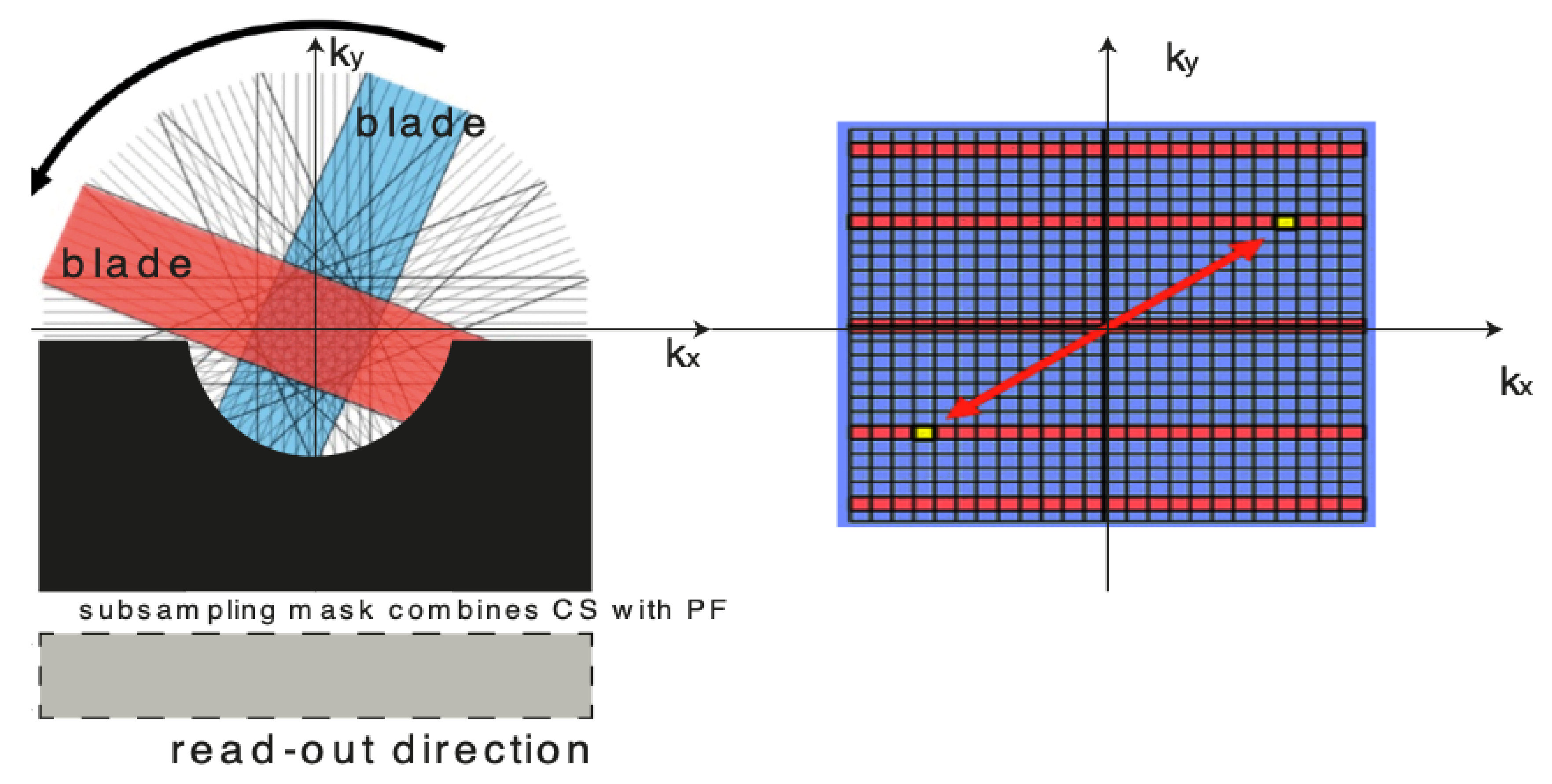
One of the possible scenarios of what could be developed is the change of phase encoding intervals in k-space filling. Unfortunately, weakened image quality can be a result. Yet, weakened image quality could be surmounted by utilising the proposed k-space sampling pattern. The sampling scheme suggested in this paper combines PROPELLER (Periodically Rotated Overlapping ParallEL Lines with Enhanced Reconstruction) sampling scheme [2] with Compressed Sensing and Partial Fourier, see Figure 1. The Partial Fourier framework claims that the phase changes gradually within the scanned object. Despite of the circumstances, numerous parallel imaging approaches such as SMASH (simultaneous acquisition of spatial harmonics) or SENSE (sensitivity encoding technique) [18], exploiting receiver-coil sensitivity prior knowledge is also useful in shortening the acquisition time [19]. The absent part of k-space could be salvaged by utilising its conjugate symmetry [20,21,22].

Consecutively, Compressed Sensing (CS) techniques [23], recently presented, may deliver further optimisation of sampling patterns. MRI revealed its relevance as the right place for applying CS frameworks. These methods can potentially accelerate the process to a higher level than any PI (Parallel Imaging) methods [23,24]. Numerous compressively-sensed methods have been brought into the limelight and tested. Considering the differences between several k-space sampling schemes, numerous efforts have been made to mutually utilise and associate unique, redundant knowledge achieved from various k-space sampling schemes. The combining of parallel imaging procedures with the Compressed Sensing methodology turns out to be more efficient in obtaining decreased image noise than with both the technologies used separately. In this work, the author presents a new MRI-associated method, which blends SR [2,3], deformable motion estimation with robust sampling trajectory pattern. The experimental results are promising and reveal the method’s true value.

2. MRI Sparse Sampling Schemes

The compressed sensing (CS) methodology was proposed to break the limitations of conventional sampling procedures [25,26]. The CS procedure exploits random undersampling and a sparsity-based template model image [27,28]. Over the last decade, many efforts have been made to improve diagnostic image reconstruction. Magnetic Resonance Imaging is a field of high priority because of its high examination charges. And, consequently, significant reduction of scanning times was a major reason for transplanting the CS to the field of Magnetic Resonance Imaging. Several researches have argued that the procedures such as k-t SPARSE, CS dynamic imaging [22] and k-t FOCUSS [29,30] images are compressible under a well-chosen sparsyfying transform. One of most important technological breakthroughs in medicine and healthcare was parallel imaging [22,31,32]. Currently, the majority of clinical scanners are loaded with parallel imaging methodology, and this way is the standard arrangement for numerous scanning schemes. It has been proven that scan time can be lowered by sampling a reduced number of phase encoding lines in frequency domain. Most modern clinical scanners collect input samples from several seperate receiver coil arrays [33].

Parallel imaging procedures utilise properties of these coil arrays to isolate aliased pixels in the image domain or to estimate missing k-space data exploiting knowledge of neighbouring k-space locations. Several approaches to the parallel imaging methods have been proposed [26,34]. The most prominent examples include SENSE, GRAPPA, and SPIRiT. They were all successfully applied in clinical practice. These procedures can be modified to consider irregular sampling schemes. Non-Cartesian sampling schemes deliver several valuable properties, that is, the appearance of incoherent aliasing artefacts. The latest improvements in concurrent multi-slice imaging are proposed, which utilise parallel imaging to separate images of numerous slices that have been obtained at the same time. Parallel imaging can also be applied to quicken three dimensional MRI, in which an adjacent volume is scanned rather than sequential slices. Another category of phase-constrained parallel imaging procedure makes use of both image magnitude and phase to improve reconstruction performance. Nevertheless, the robustness of compressively sensed MRI scanning procedures is still technically challenging. Numerous authors have noted that the pulse sequence is supposed to be wisely implemented to overcome any tendency of inconsistency, such as image resolution, number of frames/slices, contrast-to-noise ratio (CNR), and field of view. Meanwhile, other authors have proposed parallel imaging methods for handling dynamic Magnetic Resonance. In this way the techniques and methods which show the most effectiveness with certain types of procedures such as TSENSE and TGRAPPA [19] have been presented. They have proven their usefulness to capture 3–4 slices per heartbeat with relevant temporal and spatial resolution for diagnostic use, utilising commercially obtainable radiofrequency (RF) coil arrays. To enhance image resolution as well as the field of view, more complex and intricate methods are needed to achieve higher acceleration rates. Examples of this include procedures such as SENSE, GRAPPA and k-t-blast [35,36,37] to ensure the precision of exploiting spatiotemporal correlations in the dynamic Magnetic Resonance Imaging data either alone or in combination with coil sensitivity information. Such data sampling, as expect, gives rise, to reducing data overlapping, which delivers high acceleration rates. The most significant disadvantage is the need of dynamic learning data to set up an aliasing pattern in the frequency domain, which minimises the resulting acceleration rate. In opposite to these techniques, the CS framework relies on the assumption that a sparsely sampled frame in a known transform domain can be calculated using randomly undersampled k-space data [38] and does not need any training data.

Figure 1. Combining Compressed Sensing (CS) with exploiting the Hermitian symmetry property produces effective sampling pattern. On the right: the two k-space locations marked in yellow colour on the graph, mirror images across the origin of k-space, have identical amplitudes but opposite phases.

Figure 1. Combining Compressed Sensing (CS) with exploiting the Hermitian symmetry property produces effective sampling pattern. On the right: the two k-space locations marked in yellow colour on the graph, mirror images across the origin of k-space, have identical amplitudes but opposite phases.

3. The Proposed Algorithm

Most SRR algorithms incline to produce similar results because of oversimplified motion trajectories which do not display real biological behaviour. This is crucial in all instances of patient motion within an image, such as respiratory, heart motion, circulation, and other potentially misregistration-causing artefacts. A deformable, groupwise non-rigid image registration method for motion compensation is utilised in the algorithm being presented in this paper [39,40].

Medical image processing has experienced a variety of difficulties in the past including distortion removal, spatial resolution and examination times [41,42]. Mathematically speaking, all these aspects lead to forming a cost function, which is crucial to get accurate and better predictions.This registration algorithm had proven its competency in the Computed Tomography [43], PET/MRI as well as DW-MRI fields. The proposed SRR algorithm concurrently uses High-Resolution sparsity priors, deformable motion registration parameters as well as the MAP (maximum a posteriori) for blur estimation. The proposed SRR algorithm minimises [39,40] the cost function consisting of the HR input image ${\Gamma }_H$, motion fields $\left\{w_i\right\}$, noise level $\left\{{\theta }_i\right\}$ as well blur kernel B. The algorithm gets started with using an initial guess which yields convergence to a solution, see the pseudocode below and Figure 2 and Figure 3.

Figure 2. An initial guess estimation yields convergence to a solution.

Figure 2. An initial guess estimation yields convergence to a solution.

Input: set of Low-resolution input Magnetic Resonance Scans /each is reconstructed from a compressively sensed k-space’s blade.

• high-resolution estimate produced by → the submethod, see Figure 2.
• iterate until convergence $|{\mathsf{\Gamma }}_L^n-{\mathsf{\Gamma }}_L^{n,\mathrm{observed}}|<\epsilon$
  • Estimate noise ${\theta }_i=\frac{\alpha +N_q-1}{\beta +N_q\overline{x}}$
  • Calculated deformable image registration parameters and utilise them to align an image grid
  • Estimate blur kernel $B_x=\underset{B_x}{argmin{\theta }_0}\parallel A{M}_y{B}_x-{\mathsf{\Gamma }}_L^n\parallel +\xi \parallel \nabla B_x\parallel$
  • Enhance the high-resolution estimate ${\mathsf{\Gamma }}_H^n$
  • Repeat steps a-d until convergence, see Figure 3

Output: high-resolution Magnetic Scan.

Figure 3. The proposed algorithm flowchart.

Figure 3. The proposed algorithm flowchart.

The procedure performs image upscaling regarding the motion fields to produce a current HR image estimate. The proposed algorithm utilises a smooth kernel, which blurs the resulting image. The image is subsampled and noised to form the set of observed low-resolution images. This iterative technique is continued until the solution converges towards values that change by less than some specified tolerance threshold between successive iterations [7]. The proposed SRR algorithm can be expressed in the following way:

$${\widehat{\mathsf{\Gamma }}}_H^n=\underset{{\mathsf{\Gamma }}_H^n}{argmin{\theta }_0}\parallel DB{\mathsf{\Gamma }}_H^n-{\mathsf{\Gamma }}_L^{n,0}\parallel +g\parallel \nabla {\mathsf{\Gamma }}_H^n\parallel +\sum _{i=-N,i\ne 0}^N\parallel DB{w}_i{\mathsf{\Gamma }}_H^n-{\mathsf{\Gamma }}_L^{n,0}\parallel .$$

(1)

Note that the ${\mathsf{\Gamma }}_L^{n,0}$ represents the estimated reference initial guess related to n-th set of “compressed” PROPELLER blades, ${\mathsf{\Gamma }}_L^{n,j}$ is the i-th obtained LR frame with regard to degradation parameters, ${\mathsf{\Gamma }}_L^n$ is HR estimate, ∇ is the gradient operator, ${\widehat{\mathsf{\Gamma }}}_H^n$ is the n-th HR image estimate $D,B,w_i$ denote the down-sampling, blur kernel, deformable image registration vectors, individually. To be able to employ gradient optimisation we need to replace L1 norms with their differentiable approximations.

It should be noted that the deformable motion estimation is a prominent example of a highly non- convex optimisation problem, which is associated with several conditions that must be satisfied [44]. Moreover, this process is highly ill-conditioned tending to sensitivity regarding measurements and model errors. The motion estimation algorithm adopted in this paper is globally optimal deformable registration. That algorithm avoids using continuous optimisation because it may be prone to local minima. To overcome this advantage, discrete optimisation was applied. The frame grid is modelled as a minimum spanning tree. Instead of using gradients to find a global optimum of the cost function, it can be found rapidly using dynamic programming, which enforces the smoothness of the deformations.

The Markov Random Field (MRF) labelling is used to perform discrete optimisation, see Figure 4. In the algorithm adopted in this paper a spanning tree with minimum total edge costs is derived. The nodes $i\in P$ refer to pixels (or group of pixels) and for each node, a collection of hidden, and corresponding to the motion fields, labels are expressed as $w_i^l=\{f_i^l,g_i^l,h_i^l\}$. The algorithm, more specifically, the energy function to be optimised consists of two terms: that is, the data cost S and the pair-wise regularisation cost $R(w_i^l,w_i^m)$ for all the nodes $l-s$ associated with the nodes $m-s$:

$$E\left(w_i\right)=\sum _{i\in P}S\left(w_i^l\right)+\kappa \sum _{l,m\in N}R(w_i^l,w_i^m).$$

(2)

The cost function shown above estimates the inter-pixel correlation of a pair of images being compared. Specifically, this term does not depend on the displacements of its neighbours.

The $\kappa$ refers to a weighting parameter, which controls the influence of the regularisation term. The first component in Equation (2) denotes the data term; the second one is the regularisation term.

Figure 4. The Magnetic Resonance image registration. This procedure is applied to the entire set of the Low-Resolution images.

Figure 4. The Magnetic Resonance image registration. This procedure is applied to the entire set of the Low-Resolution images.

4. Results

In the experimental studies, all the raw data signals are appropriately compressed with the sampling rates: 25%, 40% and 60% of the fully sampled k-spaces.

In order to measure the performance of the proposed algorithm, both laboratory phantom studies and an in-vivo assessment were performed. The purpose of the experiment was to compare the effectiveness of various ways of obtaining a compressively-sensed input. In a study of the effects of various compressed-sensing ratio on test performance, the test performance of the proposed Super-Resolution Image Reconstruction method was tested. Moreover, several MRI k-space sampling patterns have been compared. Figure 5, Figure 6, Figure 7, Figure 8, Figure 9, Figure 10, Figure 11, Figure 12, Figure 13, Figure 14, Figure 15, Figure 16, Figure 17, Figure 18, Figure 19, Figure 20, Figure 21 and Figure 22 show the achieved results. It must be emphasised that combining Compressed Sensing with Hermitian symmetry property, as well as Partial Fourier allows the shortening of k-space filling when compared to the different k-space sampling schemes, see Figure 1.

Figure 5. The phantom images based on experiment results. See from the upper row: the unprocessed image corrupted by simulated shift and the reconstructed images with various sampling rates (varying from 25% to 40% and 60% of samples of the ground truth).

Figure 5. The phantom images based on experiment results. See from the upper row: the unprocessed image corrupted by simulated shift and the reconstructed images with various sampling rates (varying from 25% to 40% and 60% of samples of the ground truth).

Figure 6. A brain imaging example. From left to right: A: Image reconstructed from partially sampled PROPELLER blade, B:Cartesian sampling grid without image registration applied (with no downsampling applied), C: B-spline Cubic interpolation, D: Non-Rigid Multi-Modal 3D Medical Image Registration Based on Foveated Modality Independent Neighbourhood Descriptor [45], E: Enhanced deep residual networks for single image super-resolution [14], F: Image super-resolution using very deep residual channel attention networks [16], G: Residual dense network for image super-resolution [15], H: super-resolution with proposed sampling scheme and motion compensation (the proposed algorithm). Compression ratio is 50%. Please see Table 1 for the PSNR values at other compression ratios.

Figure 6. A brain imaging example. From left to right: A: Image reconstructed from partially sampled PROPELLER blade, B:Cartesian sampling grid without image registration applied (with no downsampling applied), C: B-spline Cubic interpolation, D: Non-Rigid Multi-Modal 3D Medical Image Registration Based on Foveated Modality Independent Neighbourhood Descriptor [45], E: Enhanced deep residual networks for single image super-resolution [14], F: Image super-resolution using very deep residual channel attention networks [16], G: Residual dense network for image super-resolution [15], H: super-resolution with proposed sampling scheme and motion compensation (the proposed algorithm). Compression ratio is 50%. Please see Table 1 for the PSNR values at other compression ratios.

Table 1. Stats of the Peak signal-to-noise ratio (PSNR) metrics for Figure 7. MAE abbreviation stands for Mean Average Error.

Reconstruction Method	N	M	MAE	SD	t	p
down-sampled without image registration	100	21.16	20.04	0.01	1.094	0.276
down-sampled with image registration	100	24.52	19.34	0.01	−0.779	0.438
motion corrected regular sampling scheme (without subsampling applied)	100	22.36	18.04	0.01	0.185	0.854
B-spline cubic interpolation /image registration applied/	100	23.31	18.01	0.01	0.184	0.274
Non-Rigid Multi-Modal 3D Medical Image Registration
Based on Foveated Modality Independent Neighbourhood Descriptor	100	26.33	17.22	0.01	−0.321	0.432
Enhanced deep residual networks for single image super-resolution	100	29.14	16.55	0.01	−0.362	0,412
Image super-resolution using very deep residual channel attention networks	100	28.75	15.51	0.01	−0.416	0.437
Residual dense network for image SR	100	29.88	14.63	0.01	−0.541	0.554
the proposed method	100	30.39	14.02	0.01	−0.588	0.558

Table 1. Stats of the Peak signal-to-noise ratio (PSNR) metrics for Figure 7. MAE abbreviation stands for Mean Average Error.

Reconstruction Method	N	M	MAE	SD	t	p
down-sampled without image registration	100	21.16	20.04	0.01	1.094	0.276
down-sampled with image registration	100	24.52	19.34	0.01	−0.779	0.438
motion corrected regular sampling scheme (without subsampling applied)	100	22.36	18.04	0.01	0.185	0.854
B-spline cubic interpolation /image registration applied/	100	23.31	18.01	0.01	0.184	0.274
Non-Rigid Multi-Modal 3D Medical Image Registration
Based on Foveated Modality Independent Neighbourhood Descriptor	100	26.33	17.22	0.01	−0.321	0.432
Enhanced deep residual networks for single image super-resolution	100	29.14	16.55	0.01	−0.362	0,412
Image super-resolution using very deep residual channel attention networks	100	28.75	15.51	0.01	−0.416	0.437
Residual dense network for image SR	100	29.88	14.63	0.01	−0.541	0.554
the proposed method	100	30.39	14.02	0.01	−0.588	0.558

Figure 7. The brain imaging results. From left to right: A: Image reconstructed from partially sampled PROPELLER blade, B:Cartesian sampling grid without image registration applied (with no downsampling applied), C: B-spline Cubic interpolation, D: Non-Rigid Multi-Modal 3D Medical Image Registration Based on Foveated Modality Independent Neighbourhood Descriptor [45], E: Enhanced deep residual networks for single image super-resolution [14], F: Image super-resolution using very deep residual channel attention networks [16], G: Residual dense network for image super-resolution [15], H: super-resolution with proposed sampling scheme and motion compensation (the proposed algorithm). Compression ratio is 50%. Please see Table 2 for the PSNR values at other compression ratios.

Figure 7. The brain imaging results. From left to right: A: Image reconstructed from partially sampled PROPELLER blade, B:Cartesian sampling grid without image registration applied (with no downsampling applied), C: B-spline Cubic interpolation, D: Non-Rigid Multi-Modal 3D Medical Image Registration Based on Foveated Modality Independent Neighbourhood Descriptor [45], E: Enhanced deep residual networks for single image super-resolution [14], F: Image super-resolution using very deep residual channel attention networks [16], G: Residual dense network for image super-resolution [15], H: super-resolution with proposed sampling scheme and motion compensation (the proposed algorithm). Compression ratio is 50%. Please see Table 2 for the PSNR values at other compression ratios.

Table 2. Stats of the Image Enhancement Metric (IEM) metrics for Figure 7.

Reconstruction Method	N	M	SD	t	p
down-sampled without image registration	100	1.76	0.01	1.222	0.225
down-sampled with image registration	100	1.99	0.01	0.505	0.615
motion corrected regular sampling scheme (without subsampling applied)	100	2.67	0.01	1.848	0.068
B-spline cubic interpolation /image registration applied/	100	2.01	0.01	0.184	0.273
Non-Rigid Multi-Modal 3D Medical Image Registration
Based on Foveated Modality Independent Neighbourhood Descriptor	100	2.33	0.01	−0.320	0.436
Enhanced deep residual networks for single image super-resolution	100	2.14	0.01	−0.361	0.411
Image super-resolution using very deep residual channel attention networks	100	2.45	0.01	−0.411	0.431
Residual dense network for image SR	100	2.88	0.01	−0.543	0.552
the proposed method	100	3.99	0.00	−1.901	0.061

Table 2. Stats of the Image Enhancement Metric (IEM) metrics for Figure 7.

Reconstruction Method	N	M	SD	t	p
down-sampled without image registration	100	1.76	0.01	1.222	0.225
down-sampled with image registration	100	1.99	0.01	0.505	0.615
motion corrected regular sampling scheme (without subsampling applied)	100	2.67	0.01	1.848	0.068
B-spline cubic interpolation /image registration applied/	100	2.01	0.01	0.184	0.273
Non-Rigid Multi-Modal 3D Medical Image Registration
Based on Foveated Modality Independent Neighbourhood Descriptor	100	2.33	0.01	−0.320	0.436
Enhanced deep residual networks for single image super-resolution	100	2.14	0.01	−0.361	0.411
Image super-resolution using very deep residual channel attention networks	100	2.45	0.01	−0.411	0.431
Residual dense network for image SR	100	2.88	0.01	−0.543	0.552
the proposed method	100	3.99	0.00	−1.901	0.061

Figure 8. The abdominal image processing. From left to right: A: Image reconstructed from partially sampled PROPELLER blade, B:Cartesian sampling grid without image registration applied (with no downsampling applied), C: B-spline Cubic interpolation, D: Non-Rigid Multi-Modal 3D Medical Image Registration Based on Foveated Modality Independent Neighbourhood Descriptor [45], E: Enhanced deep residual networks for single image super-resolution [14], F: Image super-resolution using very deep residual channel attention networks [16], G: Residual dense network for image super-resolution [15], H: super-resolution with proposed sampling scheme and motion compensation (the proposed algorithm). Compression ratio is 50%. Please see Table 3 for the PSNR values at other compression ratios.

Figure 8. The abdominal image processing. From left to right: A: Image reconstructed from partially sampled PROPELLER blade, B:Cartesian sampling grid without image registration applied (with no downsampling applied), C: B-spline Cubic interpolation, D: Non-Rigid Multi-Modal 3D Medical Image Registration Based on Foveated Modality Independent Neighbourhood Descriptor [45], E: Enhanced deep residual networks for single image super-resolution [14], F: Image super-resolution using very deep residual channel attention networks [16], G: Residual dense network for image super-resolution [15], H: super-resolution with proposed sampling scheme and motion compensation (the proposed algorithm). Compression ratio is 50%. Please see Table 3 for the PSNR values at other compression ratios.

Table 3. Stats of the PSNR metrics for Figure 17. M denotes mean of observed PSNRs. MAE abbreviation stands for Mean Average Error.

Reconstruction Method	N	M	MAE	SD	t	p
Image reconstructed from partially sampled PROPELLER blade	100	19.16	19.22	0.01	1.654	0.101
no motion corrected regular sampling scheme (with no downsampling applied)	100	26.21	18.34	0.01	0.672	0.503
B-spline cubic interpolation /image registration applied/	100	23.31	17.89	0.01	0.183	0.273
Non-Rigid Multi-Modal 3D Medical Image Registration
Based on Foveated Modality Independent Neighbourhood Descriptor	100	26,22	17.02	0.01	−0.354	0.431
Enhanced deep residual networks for single image super-resolution	100	29.65	16.44	0.01	−0.384	0,411
Image super-resolution using very deep residual channel attention networks	100	28.66	16.01	0.01	−0.466	0.436
Residual dense network for image SR	100	29.00	15.55	0.01	−0.565	0.554
the proposed method	100	29.28	14.07	0.01	−1.002	0.554

Table 3. Stats of the PSNR metrics for Figure 17. M denotes mean of observed PSNRs. MAE abbreviation stands for Mean Average Error.

Reconstruction Method	N	M	MAE	SD	t	p
Image reconstructed from partially sampled PROPELLER blade	100	19.16	19.22	0.01	1.654	0.101
no motion corrected regular sampling scheme (with no downsampling applied)	100	26.21	18.34	0.01	0.672	0.503
B-spline cubic interpolation /image registration applied/	100	23.31	17.89	0.01	0.183	0.273
Non-Rigid Multi-Modal 3D Medical Image Registration
Based on Foveated Modality Independent Neighbourhood Descriptor	100	26,22	17.02	0.01	−0.354	0.431
Enhanced deep residual networks for single image super-resolution	100	29.65	16.44	0.01	−0.384	0,411
Image super-resolution using very deep residual channel attention networks	100	28.66	16.01	0.01	−0.466	0.436
Residual dense network for image SR	100	29.00	15.55	0.01	−0.565	0.554
the proposed method	100	29.28	14.07	0.01	−1.002	0.554

Figure 9. The Shepp-Logan phantom results comparison. From the left: the PROPELLER sampling reconstruction output (PSNR = 29.84 dB, IEM = 2.04), the proposed algorithm result with enhanced resolution (PSNR = 34.58 dB, IEM = 3.64). The lower row shows detailed images. Please see Table 4 for the PSNR values at other compression ratios.

Figure 9. The Shepp-Logan phantom results comparison. From the left: the PROPELLER sampling reconstruction output (PSNR = 29.84 dB, IEM = 2.04), the proposed algorithm result with enhanced resolution (PSNR = 34.58 dB, IEM = 3.64). The lower row shows detailed images. Please see Table 4 for the PSNR values at other compression ratios.

Table 4. Stats of the PSNR metrics for Table 5 at different CS ratio. M denotes mean of observed PSNRs. MAE abbreviation stands for Mean Average Error.

CS Quality [%]	N	M	MAE	SD	t(99)	p
20	100	18.76	20.01	0.01	0.647	0.519
40	100	25.62	18.08	0.01	0.799	0.426
50	100	30.39	15.01	0.01	1.848	0.068
60	100	31.16	14.04	0.01	1.222	0.225

Table 4. Stats of the PSNR metrics for Table 5 at different CS ratio. M denotes mean of observed PSNRs. MAE abbreviation stands for Mean Average Error.

CS Quality [%]	N	M	MAE	SD	t(99)	p
20	100	18.76	20.01	0.01	0.647	0.519
40	100	25.62	18.08	0.01	0.799	0.426
50	100	30.39	15.01	0.01	1.848	0.068
60	100	31.16	14.04	0.01	1.222	0.225

Table 5. Stats of the PSNR metrics for Figure 12. M denotes mean of observed PSNRs. MAE abbreviation stands for Mean Average Error.

Reconstruction Method	N	M	MAE	SD	t	p
Image reconstructed from partially sampled
PROPELLER blade	100	18.23	20.01	0.01	−0.300	0.765
no motion corrected regular sampling scheme
(with no downsampling applied)	100	26.86	19.72	0.01	−1.554	0.121
B-spline cubic interpolation /image registration applied/	100	23.30	18.91	0.01	0.181	0.275
Non-Rigid Multi-Modal 3D Medical Image Registration
Based on Foveated Modality Independent Neighbourhood Descriptor	100	26.31	1.23	0.01	−0.323	0.437
Enhanced deep residual networks for single image super-resolution	100	29.41	16.00	0.01	−0.367	0.411
Image super-resolution using very deep residual channel
attention networks	100	28.12	15.61	0.01	−0.412	0.432
Residual dense network for image SR	100	29.93	15.01	0.01	−0.542	0.558
the proposed method	100	36.22	14.32	0.01	1.347	0.181

Table 5. Stats of the PSNR metrics for Figure 12. M denotes mean of observed PSNRs. MAE abbreviation stands for Mean Average Error.

Reconstruction Method	N	M	MAE	SD	t	p
Image reconstructed from partially sampled
PROPELLER blade	100	18.23	20.01	0.01	−0.300	0.765
no motion corrected regular sampling scheme
(with no downsampling applied)	100	26.86	19.72	0.01	−1.554	0.121
B-spline cubic interpolation /image registration applied/	100	23.30	18.91	0.01	0.181	0.275
Non-Rigid Multi-Modal 3D Medical Image Registration
Based on Foveated Modality Independent Neighbourhood Descriptor	100	26.31	1.23	0.01	−0.323	0.437
Enhanced deep residual networks for single image super-resolution	100	29.41	16.00	0.01	−0.367	0.411
Image super-resolution using very deep residual channel
attention networks	100	28.12	15.61	0.01	−0.412	0.432
Residual dense network for image SR	100	29.93	15.01	0.01	−0.542	0.558
the proposed method	100	36.22	14.32	0.01	1.347	0.181

Figure 10. The bee swarm plots are one-dimensional scatter plots showing the “stripcharts” of the PSNR scores for all the methods on each dataset from Figure 7.

Figure 10. The bee swarm plots are one-dimensional scatter plots showing the “stripcharts” of the PSNR scores for all the methods on each dataset from Figure 7.

Figure 11. The beeswarm* plots are one-dimensional scatter plots showing the “stripcharts” of the IEM scores for all the methods on each dataset from Figure 7. *The so-called bee swarm plot gives a better representation of the distribution of values, but it does not scale well to large numbers of observations.

Figure 11. The beeswarm* plots are one-dimensional scatter plots showing the “stripcharts” of the IEM scores for all the methods on each dataset from Figure 7. *The so-called bee swarm plot gives a better representation of the distribution of values, but it does not scale well to large numbers of observations.

Figure 12. The bee swarm plots are one-dimensional scatter plots showing the “stripcharts” of the PSNR scores for all the methods on each dataset from Figure 7 (Table 4 illustrated).

Figure 12. The bee swarm plots are one-dimensional scatter plots showing the “stripcharts” of the PSNR scores for all the methods on each dataset from Figure 7 (Table 4 illustrated).

Figure 13. The bee swarm plots are one-dimensional scatter plots showing the “stripcharts” of the IEM scores for all the methods on each dataset from Figure 7 (Table 6 illustrated).

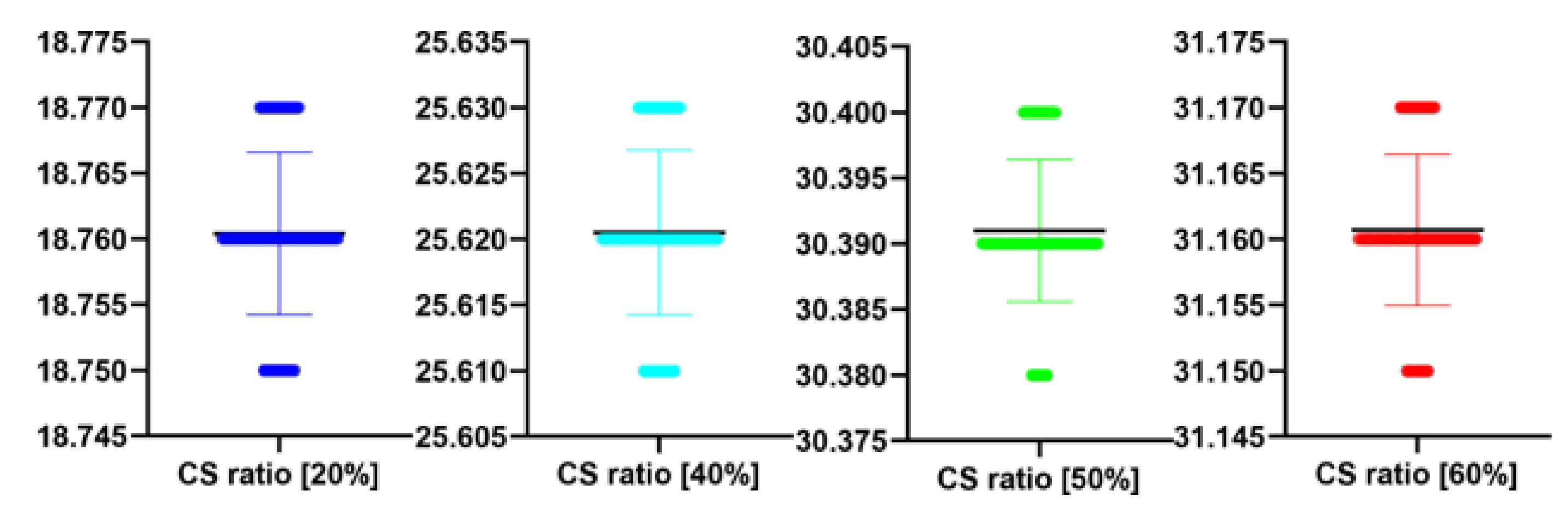
Figure 13. The bee swarm plots are one-dimensional scatter plots showing the “stripcharts” of the IEM scores for all the methods on each dataset from Figure 7 (Table 6 illustrated).

Table 6. Stats of the IEM metrics for Figure 7 at different CS ratio.

CS Quality [%]	N	IEM	SD	t(99)	p
20	100	1.79	0.00	−1.421	0.158
40	100	1.88	0.01	1.654	0.101
50	100	3.99	0.01	−1.179	0.241
60	100	4.31	0.00	0.000	1.000

Table 6. Stats of the IEM metrics for Figure 7 at different CS ratio.

CS Quality [%]	N	IEM	SD	t(99)	p
20	100	1.79	0.00	−1.421	0.158
40	100	1.88	0.01	1.654	0.101
50	100	3.99	0.01	−1.179	0.241
60	100	4.31	0.00	0.000	1.000

Figure 14. The bee swarm plots are one-dimensional scatter plots showing the “stripcharts” of the PSNR scores for all the methods on each dataset from Figure 12.

Figure 14. The bee swarm plots are one-dimensional scatter plots showing the “stripcharts” of the PSNR scores for all the methods on each dataset from Figure 12.

Figure 15. The bee swarm plots are one-dimensional scatter plots showing the “stripcharts” of the IEM scores for all the methods on each dataset from Figure 12.

Figure 15. The bee swarm plots are one-dimensional scatter plots showing the “stripcharts” of the IEM scores for all the methods on each dataset from Figure 12.

Figure 16. The bee swarm plots are one-dimensional scatter plots showing the “stripcharts” of the PSNR scores for all the methods on each dataset from Figure 12.

Figure 16. The bee swarm plots are one-dimensional scatter plots showing the “stripcharts” of the PSNR scores for all the methods on each dataset from Figure 12.

Figure 17. The bee swarm plots are one-dimensional scatter plots showing the “stripcharts” of the IEM scores for all the methods on each dataset from Figure 12.

Figure 17. The bee swarm plots are one-dimensional scatter plots showing the “stripcharts” of the IEM scores for all the methods on each dataset from Figure 12.

Figure 18. The bee swarm plots are one-dimensional scatter plots showing the “stripcharts” of the PSNR scores for all the methods on each dataset from Figure 18.

Figure 18. The bee swarm plots are one-dimensional scatter plots showing the “stripcharts” of the PSNR scores for all the methods on each dataset from Figure 18.

Figure 19. The bee swarm plots are one-dimensional scatter plots showing the “stripcharts” of the IEM scores for all the methods on each dataset from Figure 17.

Figure 19. The bee swarm plots are one-dimensional scatter plots showing the “stripcharts” of the IEM scores for all the methods on each dataset from Figure 17.

Figure 20. The bee swarm plots are one-dimensional scatter plots showing the “stripcharts” of the PSNR scores for all the methods on each dataset from Figure 17.

Figure 20. The bee swarm plots are one-dimensional scatter plots showing the “stripcharts” of the PSNR scores for all the methods on each dataset from Figure 17.

Figure 21. The bee swarm plots are one-dimensional scatter plots showing the “stripcharts” of the IEM scores for all the methods on each dataset from Figure 17.

Figure 21. The bee swarm plots are one-dimensional scatter plots showing the “stripcharts” of the IEM scores for all the methods on each dataset from Figure 17.

It must be emphasised that combining Compressed Sensing with Hermitian symmetry property, as well as Partial Fourier allows the shortening of k-space filling when compared to the different k-space sampling schemes. This paper focuses on fusing the super-resolution image reconstruction with k-space sparse sampling of MRI scanners. Moreover, the phantom studies were concentrated on the inverse problems of compressed sensing for MRI, see Figure 9. In this part of the experiment the Shepp-Logan phantom data Figure 6 and Figure 22 were reconstructed from sets of sparse projections. To model the sparsity, PROPELLER blades have been sensitively compressed with 30 and twelve radial lines in frequency domain as well as reconstruction from reduced-angle projections, with a contracted subset of 50 projections within a 90-degree aperture. The unmodified PROPELLER sampling scheme has been compared with the proposed one, see Figure 23. Furthermore, the ground truth MR images meshes were warped using nonrigid, deformable transformations. Lastly, Gaussian blur kernel and noise and downsampling were applied to such processed images to simulate real MR images.

Figure 22. The bee swarm plots are one-dimensional scatter plots showing the “stripcharts” of the PSNR scores for all the methods on each dataset from Figure 22.

Figure 22. The bee swarm plots are one-dimensional scatter plots showing the “stripcharts” of the PSNR scores for all the methods on each dataset from Figure 22.

Figure 23. The bee swarm plots are one-dimensional scatter plots showing the “stripcharts” of the IEM scores for all the methods on each dataset from Figure 22.

Figure 23. The bee swarm plots are one-dimensional scatter plots showing the “stripcharts” of the IEM scores for all the methods on each dataset from Figure 22.

5. Discussion

For over nearly two decades, SR procedures have effectively been exploited to enhance the spatial resolution of diagnostic images after k-spaces data are collected, thus making the doctor’s diagnosis easier. The variety of applications and methods has grown ever since, especially in the MRI modality, exposing the interest of the community to such post- processing. MRI, CT, PET and hybrid techniques are still suffering from insufficient spatial resolution, contrast issues, visual noise scattering and blurring produced by motion artefacts. These underlying issues can lead to problems in identifying abnormalities. Reducing scanning time is a serious challenge for many medical imaging techniques. Compressed Sensing (CS) theory delivers an appealing framework to address this inconvenience since it provides theoretical guarantees on the reconstruction of sparse signals by projection on a low dimensional linear subspace. Numerous adjustments here are presented and proven to be efficient for enhancing MRI spatial resolution while reducing acquisition lengths. The proposed technique minimises artefacts produced by highly sparse data, even in the influence of misregistration artefacts. In order to expedite the process of k-space filling and enhance spatial resolution, the algorithm combines several sub-techniques, that is, compressive-sensing, Poisson Disc sampling and Partial Fourier with SR technique. This combination allowed for improving both image definition and time consumption. Furthermore, improved upper frequencies provides better edge delineation. The proposed algorithm can be directly implemented to MR scanners without any hardware modifications. Moreover, it has been proven that the implemented technique produces enhanced and sharper shapes. It really minimises the risk of misdiagnosis. The financial aspects in healthcare must be addressed and sufficient value to all participants are supposed to justify their use. Apart from enhancing the spatial resolution, this technique can be useful in addressing misregistration issues. Phantom-based studies as well in-vivo experiments have proven to be successful in reducing examination time. The achieved results show an improvement of definition and readability of the MR images, see Figure 5, Figure 6, Figure 7, Figure 8, Figure 9, Figure 10, Figure 11, Figure 12, Figure 13, Figure 14, Figure 15, Figure 16, Figure 17, Figure 18, Figure 19, Figure 20, Figure 21, Figure 22 and Figure 23. The techniques used to identify abnormalities that are claimed to be potentially malignant or pre-malignant expose a higher capability to spot them due to the improved image quality parameters. Furthermore, the achievements have been validated by PSNR and IEM metrics [45] that can measure medical image quality with great competence. In more extended studies numerous scanning techniques were investigated. The proposed algorithm has been compared with SENSE, GRAPPA as well as unmodified PROPELLER. Despite reasonable results achieved using competitive algorithms, the proposed algorithms offered the shortest scanning time, see Table 7. In order to get a quantitative assessment, the peak signal-to-noise ratio (PSNR) and the mean absolute error (MAE) have been utilised. Both the smaller MAE or higher PSNR confirmed robustness of the applied algorithm. All the most commonly applied image quality metrics, including the IEM, confirmed the weight of the results. The proposed algorithm was compared with 4 state-of-the-art SRRs: Non-Rigid Multi-Modal 3D Medical Image Registration Based on Foveated Modality Independent Neighbourhood Descriptor [45], Residual dense network for image super-resolution [15], Enhanced deep residual networks for single image super-resolution [14] and Image super-resolution using very deep residual channel attention networks [16]. L1-cost regularisation is applied to learn the nets of the following procedures—Enhanced deep residual networks for single image super-resolution, Residual dense network for image super-resolution and Image super-resolution using very deep residual channel attention networks. The compressively-sensed, Super-Resolution images have achieved the highest IEM values [46]. it is obvious to see that the compression ratios highly affect the PSNR scores (see Table 1, Table 2, Table 3, Table 4, Table 5, Table 6, Table 7, Table 8, Table 9, Table 10, Table 11, Table 12, Table 13, Table 14, Table 15, Table 16, Table 17 and Table 18). It is worth being underlined that satisfying results occurred for halved sampling spaces. The mean PSNR and IEM values are used to compare the results. Each simulation was run N = 100 times. The signed rank test was applied to all the image quality metrics to verify if the null hypothesis that the central tendency of the difference was zero at numerous acceleration rates. All the statistical tests were performed using The R Project for Statistical Computing, see Figure 10, Figure 11, Figure 12, Figure 13, Figure 14, Figure 15, Figure 16, Figure 17, Figure 18, Figure 19, Figure 20, Figure 21, Figure 22 and Figure 23. A separate group t-student‘s test was conducted in order to compare the PSNR mean scores between 2 seperate sets, with a paired t-test. The significance test, Student’s t-test was carried out on the PSNR and are found that the probability validates the method’s performance. The results are exposed in Table 1, Table 2, Table 3, Table 4, Table 5, Table 6, Table 7, Table 8, Table 9, Table 10, Table 11, Table 12, Table 13, Table 14, Table 15, Table 16, Table 17, Table 18 and Table 19. The achieved p-values have proven high statistical significance. Future research will be concentrated on testing competitive solutions which operate using Discrete Shearlet Transform because of its ability to be a good candidate for MRI sparse sampling. Presently, the algorithm is being validated via testing using DW-MRI/PET scanners.

Table 7. Comparison of the scanning parameters

Scanning Pattern	TR	TE	FOV	Voxel (mm)	Total Scan Duration (s)	p
PROPELLER	1200	180	290	0.96/0.96/1.00	360	0.159
SENSE	1200	180	290	0.96/0.96/1.00	353	0.226
GRAPPA	1200	180	290	0.96/0.96/1.00	320	0.136
the proposed algorithm	1200	180	290	0.96/0.96/1.00	112	0.103

Table 7. Comparison of the scanning parameters

Scanning Pattern	TR	TE	FOV	Voxel (mm)	Total Scan Duration (s)	p
PROPELLER	1200	180	290	0.96/0.96/1.00	360	0.159
SENSE	1200	180	290	0.96/0.96/1.00	353	0.226
GRAPPA	1200	180	290	0.96/0.96/1.00	320	0.136
the proposed algorithm	1200	180	290	0.96/0.96/1.00	112	0.103

Table 8. The performance of the proposed algorithm at different CS ratio. MAE abbreviation stands for Mean Average Error.

CS Ratio [%]	PSNR [dB]	MAE	IEM
20	18.76	19.82	1.79
40	25.62	18.01	1.88
50	30.39	15.66	3.99
60	31.16	14.20	4.31

Table 8. The performance of the proposed algorithm at different CS ratio. MAE abbreviation stands for Mean Average Error.

CS Ratio [%]	PSNR [dB]	MAE	IEM
20	18.76	19.82	1.79
40	25.62	18.01	1.88
50	30.39	15.66	3.99
60	31.16	14.20	4.31

Table 9. Stats of the IEM metrics for Figure 12. M denotes mean of observed IEMs

Reconstruction Method	N	M	SD	t	p
Image reconstructed from partially sampled
PROPELLER blade	100	1.56	0.01	1.133	0.260
no motion corrected regular sampling scheme
(with no downsampling applied)	100	3.12	0.01	0.294	0.070
B-spline cubic interpolation /image registration applied/	100	2.62	0.01	1.842	0.061
Non-Rigid Multi-Modal 3D Medical Image Registration
Based on Foveated Modality Independent Neighbourhood Descriptor	100	2.11	0.01	0.183	0.275
Enhanced deep residual networks for single image super-resolution	100	2.32	0.01	−0.327	0.436
Image super-resolution using very deep residual channel
attention networks	100	2.15	0.01	−0.366	0.412
Residual dense network for image SR	100	2.43	0.01	−0.412	0.432
the proposed method	100	2.82	0.01	−0.51	0.551
Image reconstructed from partially sampled
PROPELLER blade	100	3.89	0.01	−0.371	0.202

Table 9. Stats of the IEM metrics for Figure 12. M denotes mean of observed IEMs

Reconstruction Method	N	M	SD	t	p
Image reconstructed from partially sampled
PROPELLER blade	100	1.56	0.01	1.133	0.260
no motion corrected regular sampling scheme
(with no downsampling applied)	100	3.12	0.01	0.294	0.070
B-spline cubic interpolation /image registration applied/	100	2.62	0.01	1.842	0.061
Non-Rigid Multi-Modal 3D Medical Image Registration
Based on Foveated Modality Independent Neighbourhood Descriptor	100	2.11	0.01	0.183	0.275
Enhanced deep residual networks for single image super-resolution	100	2.32	0.01	−0.327	0.436
Image super-resolution using very deep residual channel
attention networks	100	2.15	0.01	−0.366	0.412
Residual dense network for image SR	100	2.43	0.01	−0.412	0.432
the proposed method	100	2.82	0.01	−0.51	0.551
Image reconstructed from partially sampled
PROPELLER blade	100	3.89	0.01	−0.371	0.202

Table 10. The performance of the proposed algorithm at different CS ratio for Figure 12. MAE abbreviation stands for Mean Average Error.

CS Ratio [%]	PSNR [dB]	MAE	IEM
20	18.44	20.01	1.75
40	28.42	18.03	1.92
50	36.22	16.05	3.89
60	38.11	14.55	4.31

Table 10. The performance of the proposed algorithm at different CS ratio for Figure 12. MAE abbreviation stands for Mean Average Error.

CS Ratio [%]	PSNR [dB]	MAE	IEM
20	18.44	20.01	1.75
40	28.42	18.03	1.92
50	36.22	16.05	3.89
60	38.11	14.55	4.31

Table 11. Stats of the PSNR metrics for Figure 12. M denotes mean of observed PSNRs.

CS Quality [%]	N	M	SD	t(99)	p
20	100	18.44	0.01	0.139	0.889
40	100	28.42	0.01	0.728	0.469
50	100	36.22	0.01	1.789	0.077
60	100	38.11	0.01	1.830	0.070

Table 11. Stats of the PSNR metrics for Figure 12. M denotes mean of observed PSNRs.

CS Quality [%]	N	M	SD	t(99)	p
20	100	18.44	0.01	0.139	0.889
40	100	28.42	0.01	0.728	0.469
50	100	36.22	0.01	1.789	0.077
60	100	38.11	0.01	1.830	0.070

Table 12. Stats of the IEM metrics for Figure 12. M denotes mean of observed IEMs

CS Quality [%]	N	M	SD	t(99)	p
20	100	1.75	0.01	1.000	0.329
40	100	1.92	0.01	−0.865	0.389
50	100	3.89	0.01	−0.672	0.503
60	100	4.31	0.01	0.961	0.339

Table 12. Stats of the IEM metrics for Figure 12. M denotes mean of observed IEMs

CS Quality [%]	N	M	SD	t(99)	p
20	100	1.75	0.01	1.000	0.329
40	100	1.92	0.01	−0.865	0.389
50	100	3.89	0.01	−0.672	0.503
60	100	4.31	0.01	0.961	0.339

Table 13. Stats of the IEM metrics for Figure 17. M denotes mean of observed IEMs.

Reconstruction Method	N	M	SD	t	p
Image reconstructed from partially sampled
PROPELLER blade	100	1.56	0.01	1.133	0.260
no motion corrected regular sampling scheme
(with no downsampling applied)	100	3.12	0.01	0.294	0.770
B-spline cubic interpolation /image registration applied/	100	2.62	0.01	1.822	0.021
Non-Rigid Multi-Modal 3D Medical Image Registration
Based on Foveated Modality Independent Neighbourhood Descriptor	100	2.10	0.01	0.123	0.225
Enhanced deep residual networks for single image super-resolution	100	2.31	0.01	−0.317	0.426
Image super-resolution using very deep residual channel
attention networks	100	2.12	0.01	−0.346	0.442
Residual dense network for image SR	100	2.49	0.01	−0.462	0.412
the proposed method	100	2.80	0.01	−0.511	0.521
Image reconstructed from partially sampled
PROPELLER blade	100	3.89	0.01	−0.371	0.202

Table 13. Stats of the IEM metrics for Figure 17. M denotes mean of observed IEMs.

Reconstruction Method	N	M	SD	t	p
Image reconstructed from partially sampled
PROPELLER blade	100	1.56	0.01	1.133	0.260
no motion corrected regular sampling scheme
(with no downsampling applied)	100	3.12	0.01	0.294	0.770
B-spline cubic interpolation /image registration applied/	100	2.62	0.01	1.822	0.021
Non-Rigid Multi-Modal 3D Medical Image Registration
Based on Foveated Modality Independent Neighbourhood Descriptor	100	2.10	0.01	0.123	0.225
Enhanced deep residual networks for single image super-resolution	100	2.31	0.01	−0.317	0.426
Image super-resolution using very deep residual channel
attention networks	100	2.12	0.01	−0.346	0.442
Residual dense network for image SR	100	2.49	0.01	−0.462	0.412
the proposed method	100	2.80	0.01	−0.511	0.521
Image reconstructed from partially sampled
PROPELLER blade	100	3.89	0.01	−0.371	0.202

Table 14. The performance of the proposed algorithm at different CS ratio. MAE abbreviation stands for Mean Average Error.

CS Ratio [%]	PSNR [dB]	MAE	IEM
20	19.31	20.01	1.67
40	24.14	18.23	1.91
50	29.28	16.02	3.68
60	31.08	15.65	4.19

Table 14. The performance of the proposed algorithm at different CS ratio. MAE abbreviation stands for Mean Average Error.

CS Ratio [%]	PSNR [dB]	MAE	IEM
20	19.31	20.01	1.67
40	24.14	18.23	1.91
50	29.28	16.02	3.68
60	31.08	15.65	4.19

Table 15. Stats of the PSNR metrics for Figure 17. M denotes mean of observed PSNRs.

CS Quality [%]	N	M	SD	t(99)	p
20	100	19.31	0.01	0.542	0.589
40	100	24.14	0.01	−0.713	0.478
50	100	29.28	0.01	−1.044	0.299
60	100	31.08	0.01	−1.021	0.310

Table 15. Stats of the PSNR metrics for Figure 17. M denotes mean of observed PSNRs.

CS Quality [%]	N	M	SD	t(99)	p
20	100	19.31	0.01	0.542	0.589
40	100	24.14	0.01	−0.713	0.478
50	100	29.28	0.01	−1.044	0.299
60	100	31.08	0.01	−1.021	0.310

Table 16. Stats of the IEM metrics for Figure 17. M denotes mean of observed IEMs.

CS Quality [%]	N	M	SD	t(99)	p
20	100	1.67	0.01	−0.575	0.566
40	100	1.91	0.01	−0.134	0.894
50	100	3.68	0.01	0.542	0.589
60	100	4.19	0.01	0.588	0.558

Table 16. Stats of the IEM metrics for Figure 17. M denotes mean of observed IEMs.

CS Quality [%]	N	M	SD	t(99)	p
20	100	1.67	0.01	−0.575	0.566
40	100	1.91	0.01	−0.134	0.894
50	100	3.68	0.01	0.542	0.589
60	100	4.19	0.01	0.588	0.558

Table 17. Stats of the PSNR metrics for Figure 22. M denotes mean of observed PSNRs. MAE abbreviation stands for Mean Average Error.

Reconstruction/Sampling Algorithm	N	M	MAE	SD	t(99)	p
the PROPELLER sampling reconstruction	100	29.84	18.22	0.01	−1.881	0.063
the proposed algorithm	100	34.58	15..01	0.00	1.149	0.253

Table 17. Stats of the PSNR metrics for Figure 22. M denotes mean of observed PSNRs. MAE abbreviation stands for Mean Average Error.

Reconstruction/Sampling Algorithm	N	M	MAE	SD	t(99)	p
the PROPELLER sampling reconstruction	100	29.84	18.22	0.01	−1.881	0.063
the proposed algorithm	100	34.58	15..01	0.00	1.149	0.253

Table 18. Stats of the IEM metrics for Figure 22. M denotes mean of observed IEMs

Reconstruction/Sampling Algorithm	N	M	SD	t(99)	p
the PROPELLER sampling reconstruction	100	2.04	0.01	0.139	0.889
the proposed algorithm	100	3.64	0.00	−1.228	0.222

Table 18. Stats of the IEM metrics for Figure 22. M denotes mean of observed IEMs

Reconstruction/Sampling Algorithm	N	M	SD	t(99)	p
the PROPELLER sampling reconstruction	100	2.04	0.01	0.139	0.889
the proposed algorithm	100	3.64	0.00	−1.228	0.222

Table 19. The performance of the proposed algorithm at different CS ratio. MAE abbreviation stands for Mean Average Error.

CS Ratio [%]	PSNR [dB]	MAE	IEM
20	21.04	20.22	1.88
40	27.45	18.23	1.92
50	34.58	15.45	3.64
60	36.01	15.01	4.17

Table 19. The performance of the proposed algorithm at different CS ratio. MAE abbreviation stands for Mean Average Error.

CS Ratio [%]	PSNR [dB]	MAE	IEM
20	21.04	20.22	1.88
40	27.45	18.23	1.92
50	34.58	15.45	3.64
60	36.01	15.01	4.17

References

- Irani, M.; Peleg, S. Improving resolution by image registration. CVGIP Graph. Models Image Process. 1991, 53, 231–239. [Google Scholar] [CrossRef]
- Malczewski, K.; Stasinski, R. High-resolution MRI image reconstruction from a PROPELLER data set of samples. Int. J. Funct. Inform. Pers. Med. 2008, 1, 311–320. [Google Scholar] [CrossRef]
- Malczewski, K. Breaking The Resolution Limit In Medical Imaging Modalities. In Proceedings of the 2012 International Conference on Image Processing, Computer Vision, Worldcomp and Pattern Recognition (IPCV’12), Las Vegas, NV, USA, 16–19 July 2012. [Google Scholar]
- Malczewski, K.; Stasinsk, R. Super Resolution for Multimedia, Image, and Video Processing Applications. In Studies in Computational Intelligence; Springer: Berlin, Germany, 2009; Volume 231. [Google Scholar]
- Kennedy, J.A.; Israel, O.; Frenkel, A.; Bar-Shalom, R.; Azhari, H. Super-resolution in PET imaging. IEEE Trans. Med. Imaging 2006, 25, 137–147. [Google Scholar] [CrossRef]
- Freeman, W.T.; Pasztor, E.C. Learning to Estimate Scenes from Images. In Advances in Neural Information Processing Systems; Kearns, M.S., Solla, S.A., Cohn, D.A., Eds.; MIT Press: Cambridge, MA, USA, 1999; Volume 11, pp. 775–781. [Google Scholar]
- Liu, C.; Sun, D. On Bayesian Adaptive Video Super Resolution. IEEE Trans. Pattern Anal. Mach. Intell. 2013, 36, 346–360. [Google Scholar] [CrossRef] [Green Version]
- Kim, J.; Lee, J.K.; Lee, K.M. Accurate image super-resolution using very deep convolutional networks. In Proceedings of the 2016 IEEE Conference on Computer Vision and Pattern Recognition (CVPR 2016), Las Vegas, NV, USA, 27–30 June 2016; pp. 1646–1654. [Google Scholar]
- Kim, J.; Lee, J.K.; Lee, K.M. Deeply recursive convolutional network for image super-resolution. In Proceedings of the 2016 IEEE Conference on Computer Vision and Pattern Recognition, Las Vegas, NV, USA, 27–30 June 2016; pp. 1637–1645. [Google Scholar]
- Tao, X.; Gao, H.; Liao, R.; Wang, J.; Jia, J. Detail-revealing deep video super-resolution. In Proceedings of the IEEE International Conference on Computer Vision (ICCV 2017), Venice, Italy, 22–29 October 2017; pp. 4482–4490. [Google Scholar]
- Sajjadi, M.S.M.; Vemulapalli, R.; Brown, M. Frame-recurrent video super-resolution. In Proceedings of the 2018 IEEE Conference on Computer Vision and Pattern Recognition (CVPR 2018), Salt Lake City, UT, USA, 18–22 June 2018; pp. 6626–6634. [Google Scholar]
- Younghyun, J.; Seoung, W.O.; Jaeyeon, K.; Seon, J.K. Deep video super-resolution network using dynamic upsampling filters without explicit motion compensation. In Proceedings of the 2018 IEEE Conference on Computer Vision and Pattern Recognition, Salt Lake City, UT, USA, 18–22 June 2018. [Google Scholar]
- Dong, C.; Loy, C.C.; He, K.; Tang, X. Learning a Deep Convolutional Network for Image Super-Resolution. In Proceedings of the European Conference on Computer Vision (ECCV), Zurich, Switzerland, 6–12 September 2014. [Google Scholar]
- Lim, B.; Son, S.; Kim, H.; Nah, S.; Lee, K.M. Enhanced deep residual networks for single image super-resolution. In Proceedings of the 2017 IEEE Conference on Computer Vision and Pattern Recognition Workshops, Honolulu, HI, USA, 21–26 July 2017; pp. 1132–1140. [Google Scholar]
- Zhang, Y.; Tian, Y.; Kong, Y.; Fu, B.Y. Residual dense network for image super-resolution. In Proceedings of the 2018 IEEE Conference on Computer Vision and Pattern Recognition, Salt Lake City, UT, USA, 18–22 June 2018; pp. 2472–2481. [Google Scholar]
- Zhang, Y.; Li, K.; Li, K.; Wang, L.; Zhong, B.; Fu, Y. Image super-resolution using very deep residual channel attention networks. In Proceedings of the Computer Vision—ECCV 2018—15th European Conference, Munich, Germany, 8–14 September 2018; Part VII. pp. 294–310. [Google Scholar]
- Haris, M.; Shakhnarovich, G.; Ukita, N. Deep back-projection networks for super-resolution. In Proceedings of the 2018 IEEE Conference on Computer Vision and PatternRecognition, Salt Lake City, UT, USA, 18–22 June 2018; pp. 1664–1673. [Google Scholar]
- Pruessmann, K.P.; Weiger, M.; Scheidegger, M.B.; Boesiger, P. SENSE: Sensitivity encoding for fast MRI. Magn. Reson. Med. 1999, 42, 952–962. [Google Scholar] [CrossRef]
- Ding, Y.; Chung, Y.C.; Jekic, M.; Simonetti, O.P. A new approach to auto-calibrated dynamic parallel imaging based on the Karhunen-Loeve transform: KL-TSENSE and KL-TGRAPPA. Magn. Reson. Med. 2011, 65, 1786–1792. [Google Scholar] [CrossRef] [Green Version]
- Küstner, T.; Würslin, C.; Gatidis, S.; Martirosian, P.; Nikolaou, K.; Schwenzer, N.F.; Schick, F.; Yang, B.; Schmidt, H. MR image reconstruction using a combination of Compressed Sensing and partial Fourier acquisition: ESPReSSo. IEEE Trans. Med. Imaging 2016, 35, 2447–2458. [Google Scholar] [CrossRef]
- Ding, Y.; Chung, Y.C.; Jekic, M.; Simonetti, O.P. A method to assess spatially variant noise in dynamic MR image series. Magn. Reson. Med. 2010, 63, 782–789. [Google Scholar] [CrossRef] [PubMed]
- Kim, D.; Dyvorne, H.A.; Otazo, R.; Feng, L.; Sodickson, D.K.; Lee, V.S. Accelerated phase-contrast cine MRI using k-t SPARSE-SENSE. Magn. Reson. Med. 2012, 67, 1054–1064. [Google Scholar] [CrossRef] [PubMed] [Green Version]
- Pedersen, H.; Kozerke, S.; Ringgaard, S.; Nehrke, K.; Kim, W. k-t PCA: Temporally constrained k-t BLAST reconstruction using principal component analysis. Magn. Reson. Imaging 2009, 63, 706–716. [Google Scholar]
- Griswold, M.A.; Jakob, P.M.; Heidemann, R.M.; Nittka, M.; Jellus, V.; Wang, J.; Kiefer, B.; Haase, A. Generalized autocalibrating partially parallel acquisitions (GRAPPA). Magn. Reson. Med. 2002, 47, 1202–1210. [Google Scholar] [CrossRef] [PubMed] [Green Version]
- Noll, D.C.; Nishimura, D.G.; Macovski, A. Homodyne detection in magnetic resonance imaging. IEEE Trans. Med. Imaging 1991, 10, 154–163. [Google Scholar] [CrossRef] [PubMed]
- McGibney, G.; Smith, M.R.; Nichols, S.T.; Crawley, A. Quantitative evaluation of several partial Fourier Reconstruction methods used in MRI. Magn. Reson. Med. 1993, 30, 51–59. [Google Scholar] [CrossRef] [PubMed]
- Davenport, M. The Fundamentals of Compressive Sensing. IEEE Signal Processing Society Online Tutorial Library, 12 April 2013. [Google Scholar]
- Cook, R.L. Stochastic sampling in computer graphics. ACM Trans. Graph. (TOG) 1986, 5, 5172. [Google Scholar] [CrossRef]
- Jung, H.; Ye, J.C.; Kim, E.Y. Improved k-t BLAST and k-t SENSE using FOCUSS. Phys. Med. Biol. 2007, 52, 3201–3226. [Google Scholar] [CrossRef]
- He, Z.; Cichocki, A.; Zdunek, R.; Xie, S. Improved FOCUSS method with conjugate gradient iterations. IEEE Trans. Signal Process. 2009, 57, 399–404. [Google Scholar]
- Deshmane, A.; Gulani, V.; Griswold, M.A.; Seiberlich, N. Parallel MR imaging. J. Magn. Reson. Imaging 2012, 36, 55–72. [Google Scholar] [CrossRef] [Green Version]
- Feng, L.; Xu, J.; Kim, D.; Axel, L.; Sodickson, D.K.; Otazo, R. Combination of compressed sensing, parallel imaging and partial Fourier for highly-accelerated 3D first-pass cardiac perfusion MRI. In Proceedings of the 19th International Society for Magnetic Resonance in Medicine (ISMRM), Quebec, QC, Canada, 7–13 May 2011; p. 4368. [Google Scholar]
- Margosian, P.; Schmitt, F.; Purdy, D. Faster MR imaging: Imaging with half the data. Healthc. Instrum. 1986, 1, 195–197. [Google Scholar]
- Cuppen, J.; van Est, A. Reducing MR imaging time by one-sided reconstruction. Magn. Reson. Med. 1987, 5, 526–527. [Google Scholar] [CrossRef]
- Otazo, R.; Kim, D.; Axel, L.; Sodickson, D. Combination of compressed sensing and parallel imaging for highly accelerated first-pass cardiac perfusion MRI. Magn. Reson. Med. 2010, 64, 767–776. [Google Scholar] [CrossRef] [PubMed] [Green Version]
- Liang, D.; Liu, B.; Wang, J.; Ying, L. Accelerating SENSE using compressed sensing. Magn. Reson. Med. 2009, 62, 1574–1584. [Google Scholar] [CrossRef] [PubMed]
- King, K.F.; Angelos, L. SENSE image quality improvement using matrix regularization. Int. Soc. Magn. Reson. Med. 2001, 9, 1771. [Google Scholar]
- Thüring, T.; Eggers, H.; Doneva, M.; Kozerke, S. A fast Reconstruction method using Compressive Sensing and an additional phase constraint. In Proceedings of the 26th European Society for Magnetic Resonance in Medicine and Biology (ESMRMB), Antalya, Turkey, 1–3 October 2009; p. 31. [Google Scholar]
- Malczewski, K. Super-Resolution with compressively sensed MR/PET signals at its input. Inform. Med. Unlocked 2020, 18, 1–20. [Google Scholar] [CrossRef]
- Malczewski, K. Rapid Diffusion Weighted Imaging with Enhanced Resolution. Appl. Magn. Reson. 2020, 51, 221–239. [Google Scholar] [CrossRef]
- Tsai, C.M.; Nishimura, D.G. Reduced aliasing artefacts using variable density k-space sampling trajectories. Magn. Reson. Med. 2000, 43, 452–458. [Google Scholar] [CrossRef]
- Lucia, M.; Granata, G.; Ichcha, M.; Mario, M.; Mario, R. GuarracinoGlioma Grade Classification via Omics Imaging. In Proceedings of the 7th International Conference on Bioimaging, Vienna, Austria, 24–26 February 2020. [Google Scholar]
- Heinrich, M.P.; Jenkinson, M.; Brady, M.; Schnabe, J.A. Globally optimal deformable registration on a minimum spanning tree using dense displacement sampling. In International Conference on Medical Image Computing and Computer-Assisted Intervention (MICCAI 2012); Ayache, N., Delingette, H., Golland, P., Mori, K., Eds.; Springer: Berlin/Heidelberg, Germany, 2012; Part III. [Google Scholar]
- Raj, A.; Singh, G.; Zabih, R.; Kressler, B.; Wang, Y.; Schuff, N.; Weiner, M. Bayesian parallel imaging with edge-preserving priors. Magn. Reson. Med. 2007, 57, 8–21. [Google Scholar] [CrossRef] [Green Version]
- Yang, F.; Ding, M.; Zhang, X. Non-Rigid Multi-Modal 3D Medical Image Registration Based on Foveated Modality Independent Neighbourhood Descriptor. Sensors 2019, 19, 4675. [Google Scholar] [CrossRef] [Green Version]
- Jaya, V.L.; Gopikakumari, R. IEM: A New Image Enhancement Metric for Contrast and Sharpness Measurements. Int. J. Comput. Appl. 2013, 79, 1–9. [Google Scholar]
© 2020 by the author. Licensee MDPI, Basel, Switzerland. This article is an open access article distributed under the terms and conditions of the Creative Commons Attribution (CC BY) license (http://creativecommons.org/licenses/by/4.0/).
Share and Cite
MDPI and ACS Style
Malczewski, K. Fixing Acceleration and Image Resolution Issues of Nuclear Magnetic Resonance. Symmetry 2020, 12, 681. https://doi.org/10.3390/sym12040681
AMA Style
Malczewski K. Fixing Acceleration and Image Resolution Issues of Nuclear Magnetic Resonance. Symmetry. 2020; 12(4):681. https://doi.org/10.3390/sym12040681
Chicago/Turabian StyleMalczewski, Krzysztof. 2020. "Fixing Acceleration and Image Resolution Issues of Nuclear Magnetic Resonance" Symmetry 12, no. 4: 681. https://doi.org/10.3390/sym12040681
Note that from the first issue of 2016, this journal uses article numbers instead of page numbers. See further details here.