Solving the Nonlinear Boundary Layer Flow Equations with Pressure Gradient and Radiation


 and
and
Abstract
: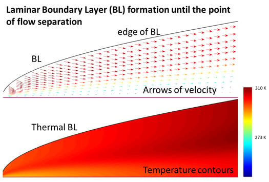
1. Introduction
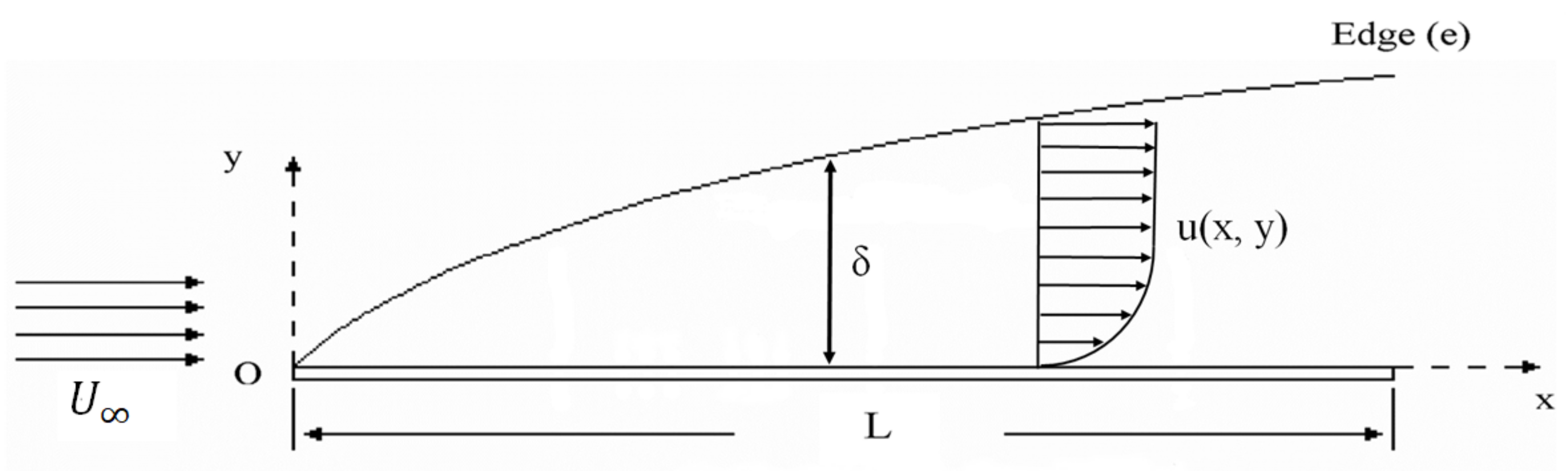
2. Mathematical Formulation
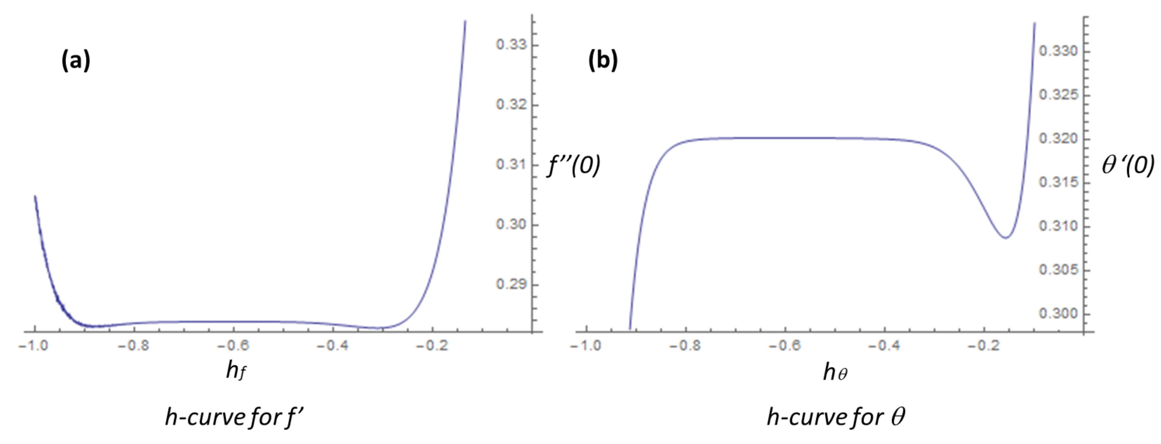
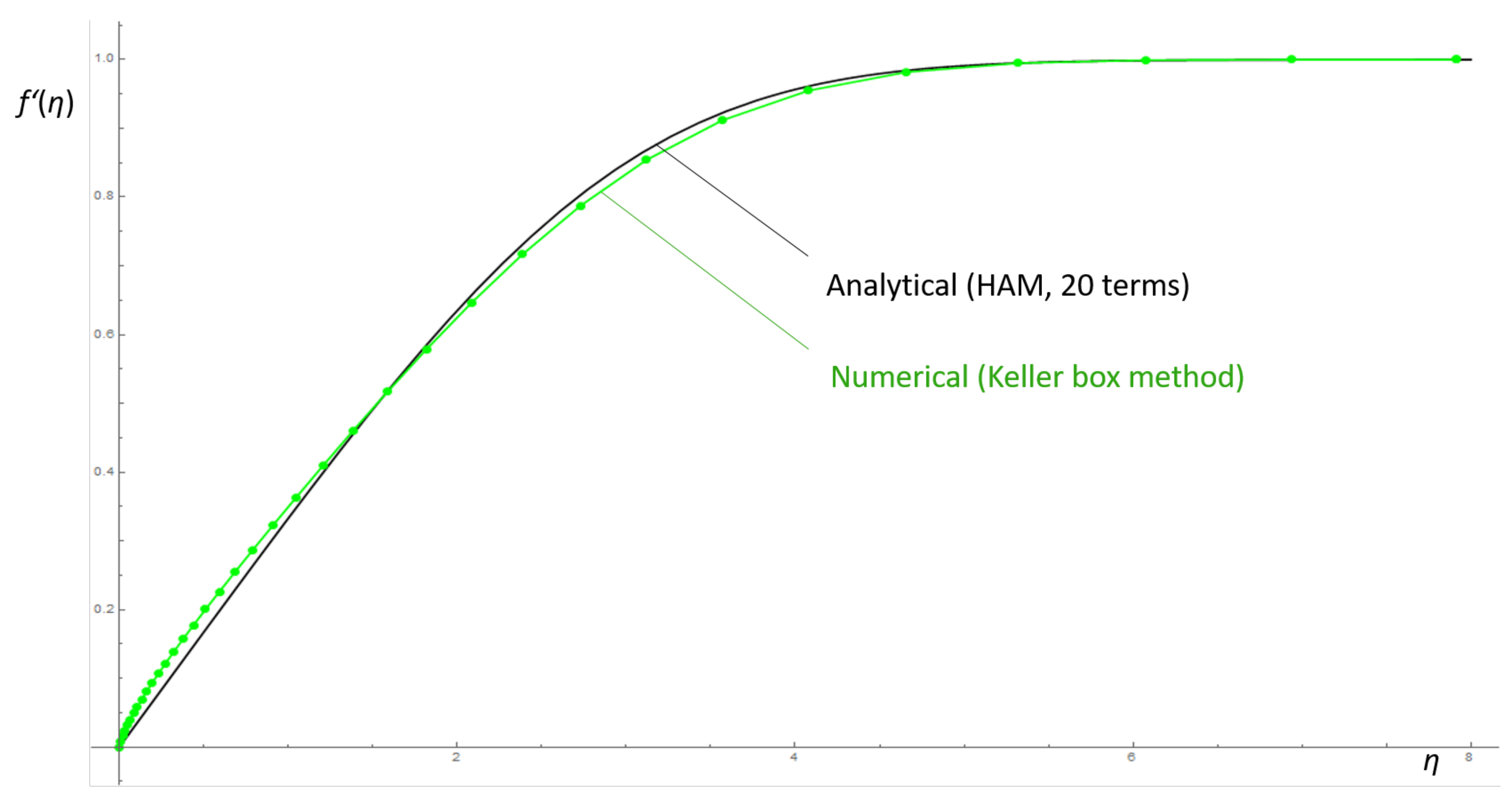
3. Application of Homotopy Analysis Method
3.1. A Short Description of HAM
- is a solution of equation
3.2. Application of HAM to System (12)–(14)
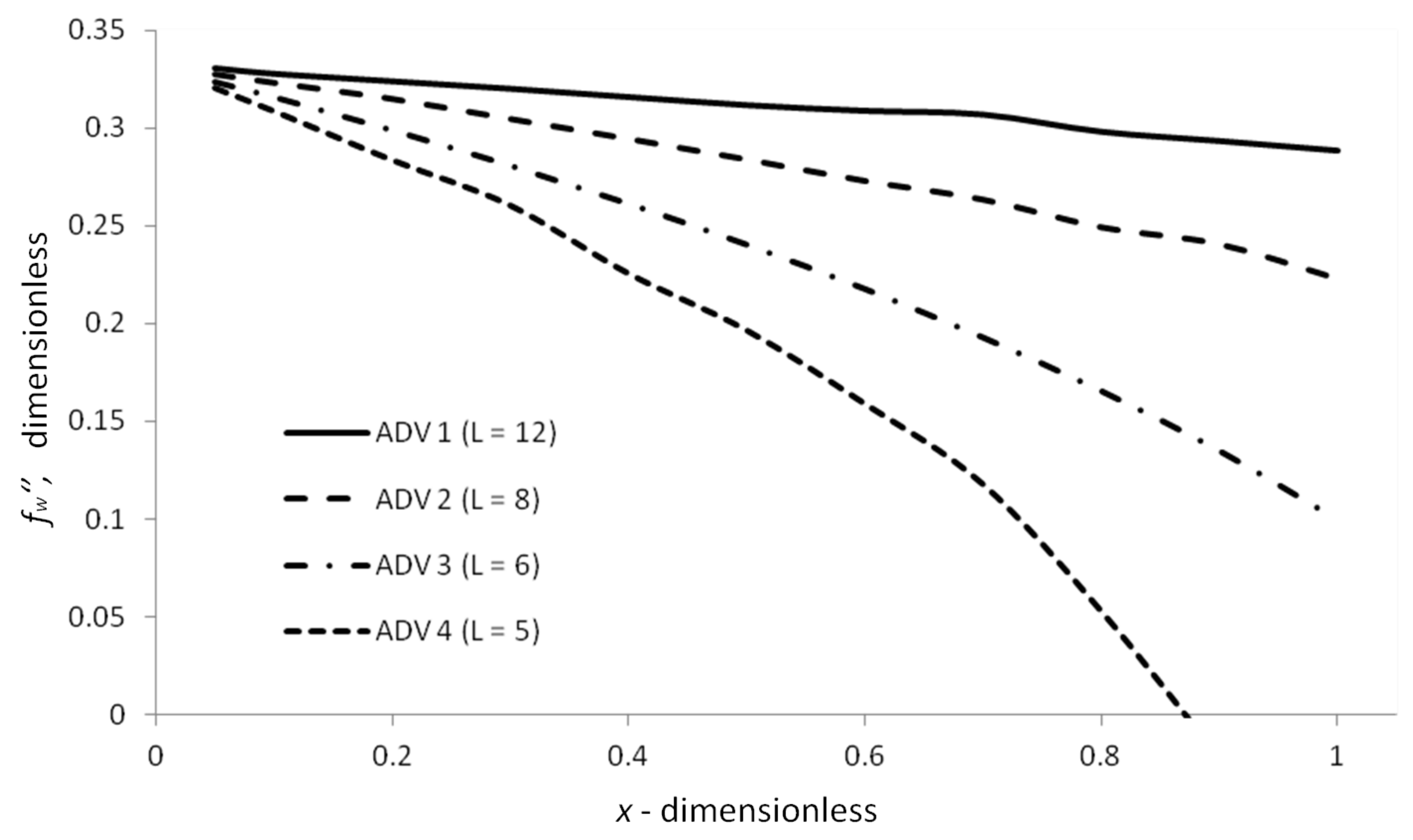
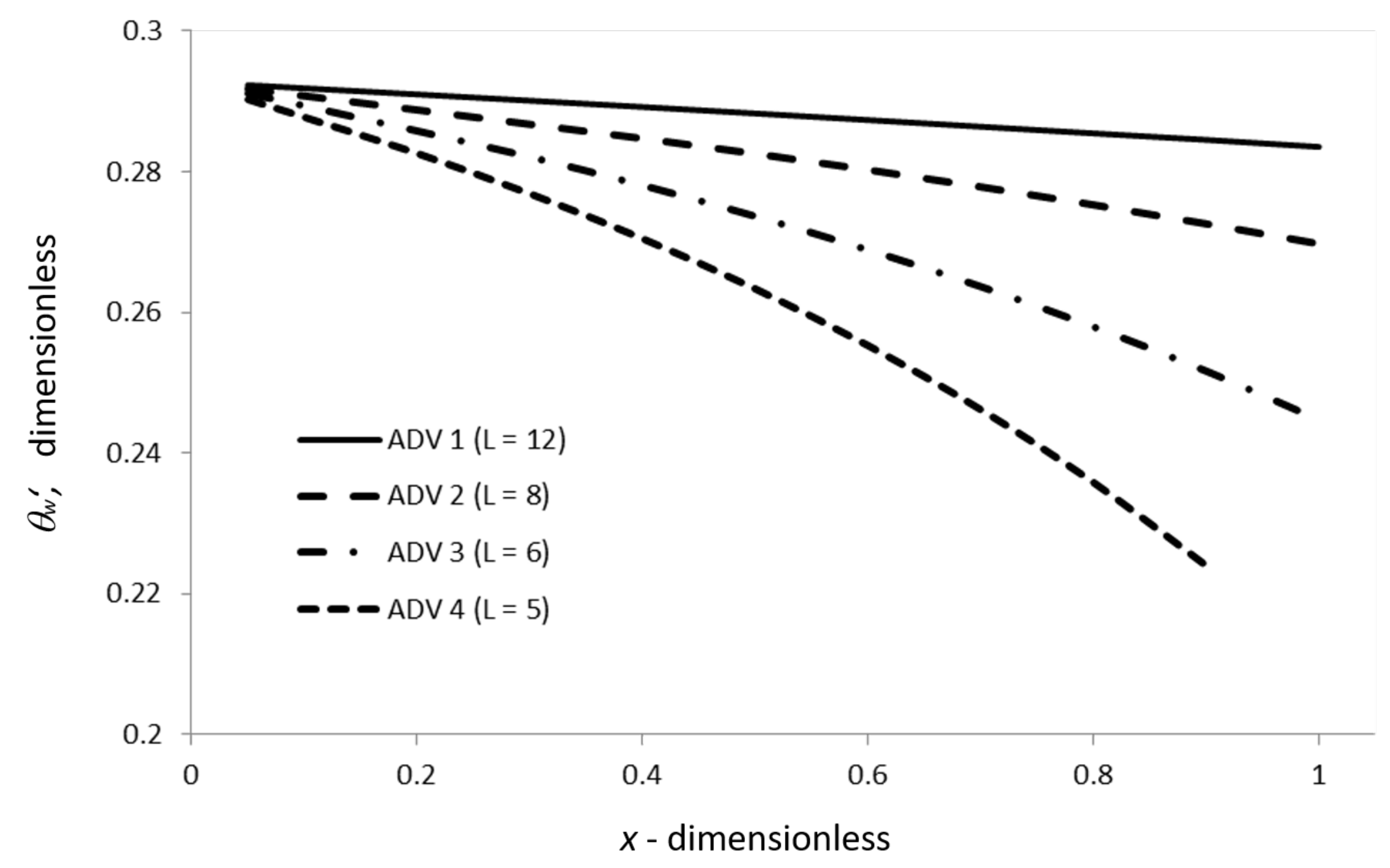
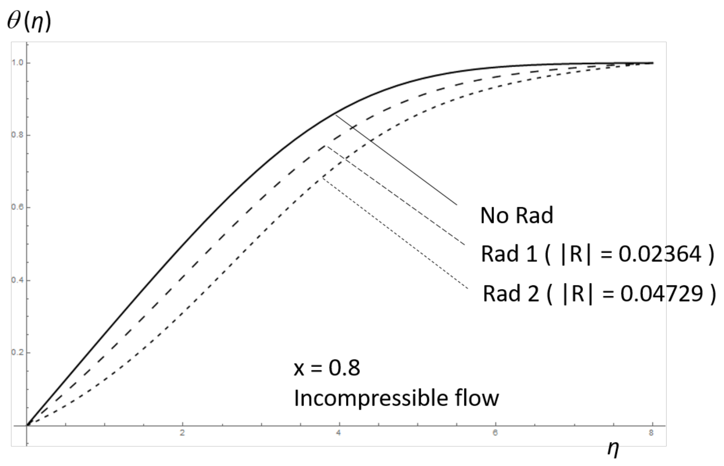
4. Results and Discussion
5. Conclusions
Author Contributions
Funding
Acknowledgments
Conflicts of Interest
Abbreviations
| PDE(s) | Partial Differential Equation(s) |
| MHD | Magnetohydrodynamic |
| HAM | Homotopy Analysis Method |
| DE(s) | Differential Equation(s) |
| ODE(s) | Ordinary Differential Equation(s) |
| APG | Adverse Pressure Gradient |
| FPG | Favorable Pressure Gradient |
| PG | Pressure Gradient |
| ADV | Adverse Pressure Effect |
| RAD | Radiation |
| e | Edge |
| coordinate system | |
| x, y | coordinates |
| free stream velocity | |
| L | length of the plate |
| dimensional boundary layer thickness | |
| u, v | dimensional velocity components of the fluid |
| density of the fluid | |
| p | pressure of the fluid |
| kinematic viscosity of the fluid | |
| dynamic viscosity of the fluid | |
| specific temperature of the fluid under constant pressure | |
| T | temperature of the fluid |
| k | coefficient of thermal conductivity |
| local radiant absorption | |
| radiative energy flux | |
| temperature of the flat plate | |
| temperature of the fluid at the edge of the boundary layer | |
| velocity of the fluid at the edge of the boundary layer | |
| absorption coefficient | |
| Stefan–Boltzmann constant | |
| dimensionless coordinate variable | |
| stream function | |
| f | dimensionless stream function |
| dimensionless temperature of the fluid | |
| Prandtl number | |
| dimensionless coordinate variable | |
| dimensionless velocity of the fluid at the edge of the boundary layer | |
| dimensionless boundary layer thickness | |
| homotopy | |
| q | embedding parameter |
| auxiliary linear operator | |
| auxiliary nonlinear operator | |
| , , | auxiliary functions |
| ℏ, , | convergence control parameters |
| set of base functions | |
| , , | “discrete square residual” errors |
| R | radiation parameter |
| local skin friction coefficient | |
| local Stanton number |
References
- Blasius, H. Grenzschichten in flüssigkeiten mit kleiner reibung. Z. Angew. Math. Phys. 1908, 56, 1–37. [Google Scholar]
- Howarth, L. On the solution of the laminar boundary layer equations. Proc. R. Soc. Lond. Ser. A 1938, 164, 547–579. [Google Scholar] [CrossRef] [Green Version]
- Cebeci, T.; Bradshaw, P. Physical and Computational Aspects of Convective Heat Transfer; Springer: New York, NY, USA, 1984. [Google Scholar]
- Howell, J.R.; Siegel, R.; Mengüç, M.P. Thermal Radiation, Heat Transfer, 5th ed.; CRC Press: Boca Raton, FL, USA, 2011. [Google Scholar]
- Kafoussias, N.; Karabis, A.; Xenos, M. Numerical study of two dimensional laminar boundary layer compressible flow with pressure gradient and heat and mass transfer. Int. J. Eng. Sci. 1999, 37, 1795–1812. [Google Scholar] [CrossRef] [Green Version]
- Kafoussias, N.; Xenos, M. Numerical study of two-dimensional turbulent boundary layer compressible flow with adverse pressure gradient and heat and mass transfer. Acta Mech. 2000, 141, 201–223. [Google Scholar] [CrossRef]
- Raptis, A.; Perdikis, C.; Takhar, H.S. Effect of thermal radiation on MHD flow. Appl. Math. Comput. 2004, 153, 645–649. [Google Scholar] [CrossRef]
- Schlichting, H.; Gersten, K. Boundary–Layer Theory, 8th ed.; Springer: Berlin, Germany, 2000. [Google Scholar]
- Raptis, A.; Perdikis, C.; Leontitsis, A. Effects of radiation in an optically thin gray gas flowing past a vertical infinite plate in the presence of magnetic field. Heat Mass Transf. 2003, 39, 771–773. [Google Scholar] [CrossRef]
- Xenos, M. Radiation Effects on flow past a stretching plate with temperature dependent viscosity. Appl. Math. 2013, 4, 1–5. [Google Scholar] [CrossRef] [Green Version]
- Ali, M.M.; Chen, T.S.; Armaly, B.F. Natural convection-radiation interaction in boundary-layer flow over horizontal surfaces. AIAA J. 1984, 22, 1797–1803. [Google Scholar] [CrossRef]
- Raptis, A.; Toki, C.J. Thermal radiation in the presence of free convective flow past a moving vertical porous plate: An analytical solution. Int. J. Appl. Mech. Eng. 2009, 14, 1115–1126. [Google Scholar]
- Raptis, A.; Perdikis, C. Radiation and free convection flow past a moving plate. Appl. Mech. Eng. 1999, 4, 817–821. [Google Scholar]
- Raptis, A.; Perdikis, C. Thermal radiation of an optically thin gray gas. Int. J. Appl. Mech. Eng. 2003, 8, 131–134. [Google Scholar]
- Seddeek, M.A.; Abdelmeguid, M.S. Effects of radiation and thermal diffusivity on heat transfer over a stretching surface with variable heat flux. Phys. Lett. A 2006, 348, 172–179. [Google Scholar] [CrossRef]
- Muthucumaraswamy, R. The interaction of thermal radiation on vertical oscillating plate with variable temperature and mass diffusion. Theor. Appl. Mech. 2006, 33, 107–121. [Google Scholar] [CrossRef] [Green Version]
- Muthucumaraswamy, R.; Chandrakala, P. Effects of thermal radiation on moving vertical plate in the presence of an optically thin gray gas. Forschung im Ingenieurwesen 2005, 69, 205–208. [Google Scholar] [CrossRef]
- Anghaie, S.; Chen, G. Application of computational fluid dynamics for thermal analysis of high temperature gas cooled and gaseous core reactors. Nucl. Sci. Eng. 1998, 130, 361–373. [Google Scholar] [CrossRef]
- Duan, L.; Martin, M.P.; Feldick, A.M.; Modest, M.F.; Levin, D.A. Study of turbulence-radiation interaction in hypersonic turbulent boundary layers. AIAA J. 2012, 50, 447–453. [Google Scholar] [CrossRef]
- Duan, L.; Martin, M.P.; Sohn, I.; Levin, D.A.; Modest, M.F. Study of emission turbulence-radiation interaction in hypersonic boundary layers. AIAA J. 2011, 49, 340–348. [Google Scholar] [CrossRef]
- Miroshnichenko, I.V.; Sheremet, M.A. Numerical simulation of turbulent natural convection combined with surface thermal radiation in a square cavity. Int. J. Numer. Methods Heat Fluid Flow 2015, 25, 1600–1618. [Google Scholar] [CrossRef]
- Miroshnichenko, I.V.; Sheremet, M.A.; Mohamad, A.A. Numerical simulation of a conjugate turbulent natural convection combined with surface thermal radiation in an enclosure with a heat source. Int. J. Therm. Sci. 2016, 109, 172–181. [Google Scholar] [CrossRef]
- Kim, S.S.; Baek, S.W. Radiation affected compressible turbulent flow over a backward facing step. Int. J. Heat Mass Transfer 1996, 39, 3325–3332. [Google Scholar] [CrossRef]
- Jawad, M.; Shah, Z.; Islam, S.; Majdoubi, J.; Tlili, I.; Khan, W.; Khan, I. Impact of nonlinear thermal radiation and the viscous dissipation effect on the unsteady three-dimensional rotating flow of single-wall carbon nanotubes with aqueous suspensions. Symmetry 2019, 11, 207. [Google Scholar] [CrossRef] [Green Version]
- Khan, S.A.; Nie, Y.; Ali, B. Multiple slip effects on magnetohydrodynamic axisymmetric buoyant nanofluid flow above a stretching sheet with radiation and chemical reaction. Symmetry 2019, 11, 1171. [Google Scholar] [CrossRef] [Green Version]
- Jamaludin, A.; Nazar, R.; Pop, I. Mixed convection stagnation-point flow of a nanofluid past a permeable stretching/shrinking sheet in the presence of thermal radiation and heat source/sink. Energies 2019, 12, 788. [Google Scholar] [CrossRef] [Green Version]
- Nayfeh, A.H. Perturbation Methods; John Wiley & Sons: Hoboken, NJ, USA, 2008. [Google Scholar]
- Dyke, M.V. Perturbation Methods in Fluid Mechanics; Parabolic Press: Stanford, CA, USA, 1975. [Google Scholar]
- Housiadas, K.D. Steady sedimentation of a spherical particle under constant rotation. Phys. Rev. Fluids 2019, 4, 103301. [Google Scholar] [CrossRef]
- Housiadas, K.D.; Ioannou, I.; Georgiou, G.C. Lubrication solution of the axisymmetric Poiseuille flow of a Bingham fluid with pressure-dependent rheological parameters. J. Non-Newton. Fluid Mech. 2018, 260, 76–86. [Google Scholar] [CrossRef]
- Housiadas, K.D.; Tanner, R.I. A high-order perturbation solution for the steady sedimentation of a sphere in a viscoelastic fluid. J. Non-Newton. Fluid Mech. 2016, 233, 166–180. [Google Scholar] [CrossRef]
- Housiadas, K.D.; Tanner, R.I. Viscoelastic shear flow past an infinitely long and freely rotating cylinder. Phys. Fluids 2018, 30, 073101. [Google Scholar] [CrossRef]
- Si, X.; Yuan, L.; Cao, L.; Zheng, L.; Shen, Y.; Li, L. Perturbation solutions for a micropolar fluid flow in a semi-infinite expanding or contracting pipe with large injection or suction through porous wall. Open Phys. 2016, 14, 231–238. [Google Scholar] [CrossRef]
- Zhang, Y.; Lin, P.; Si, X.-H. Perturbation solutions for asymmetric laminar flow in porous channel with expanding and contracting walls. Appl. Math. Mech.-Engl. Ed. 2014, 35, 203–220. [Google Scholar] [CrossRef]
- Liu, Y.; Kurra, S.N. Solution of Blasius equation by variational iteration. Appl. Math. 2011, 1, 24–27. [Google Scholar] [CrossRef] [Green Version]
- Xu, L.; Lee, E.W.M. Variational iteration method for the magnetohydrodynamic flow over a nonlinear stretching sheet. Abstr. Appl. Anal. 2013, 2013, 573782. [Google Scholar] [CrossRef]
- Abbasbandy, S. A numerical solution of Blasuis equation by Adomians decomposition method and comparison with homotopy perturbation method. Chaos Solitons Fractals 2007, 31, 257–260. [Google Scholar] [CrossRef]
- Aski, F.S.; Nasirkhani, S.J.; Mohammadiand, E.; Asgari, A. Application of Adomian decomposition method for micropolar flow in a porous channel. Prop. Power Res. 2014, 3, 15–21. [Google Scholar] [CrossRef] [Green Version]
- Kuo, B.-L. Application of the differential transformation method to the solutions of Falkner-Skan wedge flow. Acta Mech. 2003, 164, 161–174. [Google Scholar] [CrossRef]
- Thiagarajan, M.; Senthilkumar, K. DTM-Padé approximants for MHD Flow with suction/blowing. J. Appl. Fluid Mech. 2012, 6, 724–728. [Google Scholar]
- Rebenda, J.; Šmarda, Z. Convergence analysis of an iterative scheme for solving initial value problem for multidimensional partial differential equations. Comp. Math. Appl. 2015, 70, 1772–1780. [Google Scholar] [CrossRef]
- Rebenda, J.; Šmarda, Z. A differential transformation approach for solving functional differential equations with multiple delays. Commun. Nonlinear Sci. Numer. Simul. 2017, 48, 246–257. [Google Scholar] [CrossRef] [Green Version]
- Rebenda, J.; Šmarda, Z. Numerical algorithm for nonlinear delayed differential systems of nth order. Adv. Differ. Equ. 2019, 2019, 26. [Google Scholar] [CrossRef] [Green Version]
- Liao, S.J. The Proposed Homotopy Analysis Technique for the Solution of Nonlinear Problems. Ph.D. Thesis, Shanghai Jiao Tong University, Shanghai, China, 1992. [Google Scholar]
- Liao, S.J. Beyond Perturbation: Introduction to the Homotoy Analysis Method; Chapman & Hall/CRC, CRC Press LLC: Boca Raton, FL, USA, 2004. [Google Scholar]
- Liao, S.J. Homotopy Analysis Method in Nonlinear Differential Equations; Springer: Berlin, Germany, 2011. [Google Scholar]
- Liao, S.J. A kind of approximate solution technique which does not depend upon small parameters-II. An application in fluid mechanics. Int. J. Nonlin. Mech. 1997, 32, 815–822. [Google Scholar] [CrossRef]
- Liao, S.J. An explicit totally analytic solution of laminar viscous flow over a semi-infinite flat plate. Commun. Nonlinear Sci. Numer. Simul. 1999, 3, 53–57. [Google Scholar] [CrossRef]
- Liao, S.J. A uniformly valid analytic solution of 2D viscous flow past a semi-infinite flat plate. J. Fluid Mech. 1999, 385, 101–128. [Google Scholar] [CrossRef] [Green Version]
- Farooq, U.; Hayat, T.; Alsaedi, A.; Liao, S.J. Series solutions of non-similarity boundary layer flows of nano-fluids over stretching surfaces. Numer. Algor. 2015, 70, 43–59. [Google Scholar]
- Jawad, M.; Shah, Z.; Kahn, A.; Kumam, P.; Islam, S. Entropy generation and heat transfer analysis in MHD unsteady rotating flow for aqueous suspensions of carbon nanotubes with nonlinear thermal radiation and viscous dissipation effect. Entropy 2019, 21, 492. [Google Scholar] [CrossRef] [Green Version]
- Naz, R.; Noor, M.; Hayat, T.; Javed, M.; Alsaed, A. Dynamism of magnetohydrodynamic cross nanofluid with particulars of entropy generation and gyrotactic motile microorganisms. Int. Commun. Heat Mass Transf. 2020, 2020 110, 104431. [Google Scholar] [CrossRef]
- Ullah, A.; Alzahrani, E.O.; Shah, Z.; Ayaz, M.; Islam, S. Nanofluids thin film flow of Reiner-Philippoff fluid over an unstable stretching surface with Brownian motion and thermophoresis effects. Coatings 2019, 9, 21. [Google Scholar] [CrossRef] [Green Version]
- Ullah, A.; Shah, Z.; Kumam, P.; Ayaz, M.; Islam, S.; Jameel, M. Viscoelastic MHD nanofluid thin film flow over an unsteady vertical stretching sheet with entropy generation. Processes 2019, 7, 262. [Google Scholar] [CrossRef] [Green Version]
- Waqas, M.; Dogonchi, A.S.; Shehzad, S.A.; Khan, M.I.; Hayat, T.; Alsaedi, A. Nonlinear convection and joule heating impacts in magneto-thixotropic nanofluid stratified flow by convectively heated variable thicked surface. J. Molecular Liquids 2020, 300, 1111945. [Google Scholar] [CrossRef]
- Hussain, M.; Ashraf, M.; Nadeem, S.; Khan, M. Radiation effects on the thermal boundary layer flow of a micropolar fluid towards a permeable stretching sheet. J. Franklin Inst. 2013, 350, 194–210. [Google Scholar] [CrossRef]
- Sharma, R.P.; Seshadri, R.; Mishra, S.R.; Munjam, S.R. Effect of thermal radiation on magnetohydrodynamic three-dimensional motion of a nanofluid past a shrinking surface under the influence of a heat source. Heat Transfer-Asian Res. 2019, 48, 2105–2121. [Google Scholar] [CrossRef]
- Sohail, M.; Naz, R.; Abdelsalam, S.I. Application of non-Fourier double diffusions theories to the boundary-layer flow of a yield stress exhibiting fluid model. Physica A 2020, 537, 122573. [Google Scholar] [CrossRef]
- Sravanthi, C.S. Effect of heat source/sink on MHD flow due to porous rotating disk with variable thickness in the presence of cross diffusion. Heat Transf.-Asian Res. 2019, 48, 4016–4032. [Google Scholar] [CrossRef]
- Nargund, A.L.; Madhusudhan, R.; Sathyanarayana, S.B. Study of compressible fluid flow in boundary layer region by homotopy analysis method. Int. J. Latest Trend Eng. Technol. 2017, 9, 28–39. [Google Scholar]
- Xenos, M. Thermal radiation effect on the MHD turbulent compressible boundary layer flow with adverse pressure gradient, heat transfer and local suction. Open J. Fluid Dyn. 2017, 7, 1–14. [Google Scholar] [CrossRef] [Green Version]
- Xenos, M.; Pop, I. Radiation effect on the turbulent compressible boundary layer flow with adverse pressure gradient. Appl. Math. Comput. 2017, 299, 153–164. [Google Scholar] [CrossRef]


| Order | -error | -error | ||
|---|---|---|---|---|
| 2 | 0.00239722 | −0.485458 | 0.0021427 | −0.637823 |
| 4 | 0.000427796 | −0.803283 | 0.000710738 | −0.596724 |
| 6 | 0.0000874967 | −0.824688 | 0.000489771 | −0.63417 |
| 8 | 0.0000507706 | −0.892126 | 0.00045183 | −0.653759 |
| 10 | 0.0000637655 | −0.87467 | 0.000441161 | −0.681927 |
| 12 | 0.0000661033 | −0.651043 | 0.000436139 | −0.68495 |
© 2020 by the authors. Licensee MDPI, Basel, Switzerland. This article is an open access article distributed under the terms and conditions of the Creative Commons Attribution (CC BY) license (http://creativecommons.org/licenses/by/4.0/).
Share and Cite
Xenos, M.A.; Petropoulou, E.N.; Siokis, A.; Mahabaleshwar, U.S. Solving the Nonlinear Boundary Layer Flow Equations with Pressure Gradient and Radiation. Symmetry 2020, 12, 710. https://doi.org/10.3390/sym12050710
Xenos MA, Petropoulou EN, Siokis A, Mahabaleshwar US. Solving the Nonlinear Boundary Layer Flow Equations with Pressure Gradient and Radiation. Symmetry. 2020; 12(5):710. https://doi.org/10.3390/sym12050710
Chicago/Turabian StyleXenos, Michalis A., Eugenia N. Petropoulou, Anastasios Siokis, and U. S. Mahabaleshwar. 2020. "Solving the Nonlinear Boundary Layer Flow Equations with Pressure Gradient and Radiation" Symmetry 12, no. 5: 710. https://doi.org/10.3390/sym12050710