HMCTS-OP: Hierarchical MCTS Based Online Planning in the Asymmetric Adversarial Environment

Abstract

The Monte Carlo Tree Search (MCTS) has demonstrated excellent performance in solving many planning problems. However, the state space and the branching factors are huge, and the planning horizon is long in many practical applications, especially in the adversarial environment. It is computationally expensive to cover a sufficient number of rewarded states that are far away from the root in the flat non-hierarchical MCTS. Therefore, the flat non-hierarchical MCTS is inefficient for dealing with planning problems with a long planning horizon, huge state space, and branching factors. In this work, we propose a novel hierarchical MCTS-based online planning method named the HMCTS-OP to tackle this issue. The HMCTS-OP integrates the MAXQ-based task hierarchies and the hierarchical MCTS algorithms into the online planning framework. Specifically, the MAXQ-based task hierarchies reduce the search space and guide the search process. Therefore, the computational complexity is significantly reduced. Moreover, the reduction in the computational complexity enables the MCTS to perform a deeper search to find better action in a limited time. We evaluate the performance of the HMCTS-OP in the domain of online planning in the asymmetric adversarial environment. The experiment results show that the HMCTS-OP outperforms other online planning methods in this domain.

1. Introduction

It is challenging to solve large-scale planning problems. These problems suffer from the “curse of dimensionality”. Online planning algorithms (e.g., the Monte Carlo Tree Search (MCTS)) overcome this problem by avoiding calculation of the complete policy for the whole state space. Additionally, the MCTS has demonstrated excellent performance in many planning problems [1].

However, existing MCTS algorithms, including the UCT (Upper Confidence Bounds (UCB) applied to Trees) cannot efficiently cope with long-horizon planning problems with a huge state space and branching factors. The performance of the MCTS is determined by the effective search depth [2]. For long-horizon problems with a huge state space and branching factors, the MCTS needs to search deeply to cover a sufficient number of rewarded states that are far away from the root, which leads to a large computational overhead and poor performance.

In this work, we focus on the online planning problem in the asymmetric adversarial environment. This domain has asymmetric military forces between two opposing players. Due to the long planning horizon, huge state space, and significant disparity among forces of this domain, the planning problem in this domain is very challenging for the MCTS.

In order to improve the performance of the MCTS, the task hierarchies or macro actions are introduced into planning [1] to reduce the computational cost. We define the set of primitive actions as A, the set of hierarchical tasks (subtasks) as $\tilde{A}$, the planning horizon as T, and the upper-bound on the length of each subtask as L. Once the primitive actions in the MCTS are replaced by the high-level subtasks, the computational cost is reduced from $O({\left|A\right|}^T)$ to $O({|\tilde{A}|}^{T/L})$ [3]. Therefore, the integration of the task hierarchies and the MCTS algorithm make the algorithm more effective for solving large-scale problems with a long planning horizon.

In this work, we use MAXQ [4] to formalize the task hierarchies. MAXQ is a decomposition method of Markov Decision Process (MDP) value function, which makes the value function representation more compact and makes the subtasks portable.

In this paper, we propose a novel hierarchical MCTS-based online planning method named the HMCTS-OP. The HMCTS-OP integrates the MAXQ-based task hierarchies and the hierarchical MCTS algorithms into the online planning framework. Specifically, the MAXQ-based task hierarchies reduce the search space and guide the search process. Therefore, the computational cost is significantly reduced, which enables the MCTS to perform a deeper search in a limited time frame. Therefore, it can provide a more accurate value function estimate for the root node and enable the root node to implement better action selection policies within the limited time frame. Moreover, combined with the advantages of hierarchical planning and online planning, the HMCTS-OP facilitates the design and utilization of autonomous agents in the asymmetric adversarial environment.

The main contributions of this paper are as follows:

• We model the online planning problem in the asymmetric adversarial environment as an MDP and extend the MDP to the semi-Markov decision process (SMDP) by introducing the task hierarchies. This provides the theoretical foundation for MAXQ hierarchical decomposition.
• We derive the MAXQ value hierarchical decomposition for the defined hierarchical tasks. The MAXQ value hierarchical decomposition provides a scalable way to calculate the rewards of hierarchical tasks in HMCTS-OP.
• We use the MAXQ-based task hierarchies to reduce the search space and guide the search process. Therefore, the computational cost is significantly reduced, which enables the MCTS to search deeper to find better action within a limited time frame. As a result, the HMCTS-OP can perform better in online planning in the asymmetric adversarial environment.

The rest of this paper is structured as follows. In Section 2, we start by introducing the necessary background. Section 3 summarizes the related work. Section 4 discusses, in detail, how to model the problem, extend the MDP to SMDP, and integrate the MAXQ-based task hierarchies in the MCTS for online planning in the asymmetric adversarial environment. In Section 5, we evaluate the performance of HMCTS-OP. In Section 6, we draw conclusions and discuss several future research areas.

2. Background

2.1. Markov and Semi-Markov Decision Process

The Markov Decision Process (MDP) is a fundamental formalism for learning and planning problems. It is defined by a four-tuple (S, A, R, P) with states S, actions A, a transition function P, and a reward function R. In general, $P(s^{\prime }|s,a)$ represents the probability of performing action $a$ in state $s$ and transitioning to state $s^{\prime }$. $R(s^{\prime }|s,a)\in ℝ$ is the reward for the state transition from s to s’ after performing action $a$. Moreover, the probability of selecting action $a$ in state s is represented as $\pi (a|s)$.

The semi-Markov decision process (SMDP) is a generalization of the MDP. In the SMDP, the actions are allowed to take variable time steps [4,5]. Let $k\in \mathbb{N}+$ denote the positive execution time of action $a$ from state s. When action $a$ is executed, the transition function $P(s^{\prime },k|s,a)$ represents the probability of performing action $a$ in state $s$ and transitioning to state $s^{\prime }$ after time $k$, and the reward function $R(s^{\prime },k|s,a)$ is the reward of the state transition from s to s′ after execution action $a$ and after time $k$. The framework of the SMDP is the foundation of hierarchical planning and learning.

2.2. MAXQ

The MAXQ value function hierarchical decomposition was proposed by Dietterich et al. [4]. MAXQ is an instance of the SMDP formulation. The fundamental action of MAXQ is to decompose a large MDP into a series of small subtasks $\left\{M_0,M_1,M_2,\dots ,M_n\right\}$. In these subtasks, each subtask is actually a sub-SMDP. All subtasks constitute a task graph, and multiple subtask policies can be learned concurrently [4]. The characteristics of the MAXQ-based task hierarchies include temporal abstraction, state abstraction, and subtask sharing. Figure 1 shows a graphic example of MAXQ-based task hierarchies.

$M_i$ is defined as a three-tuple $\langle T_i,A_i,{\tilde{R}}_i\rangle$.

• $T_i$ represents the termination condition of subtask $M_i$, which is used to judge whether $M_i$ is terminated. Specifically, $S_i$ and $G_i$ are the active states and termination states of $M_i$ respectively. If the current state $s\in G_i$ or the predefined maximum calculation time or number of iterations is reached, $T_i$ is set to 1, indicating that $M_i$ is terminated.
• $A_i$ is a set of actions; it contains both primitive actions and high-level subtasks.
• ${\tilde{R}}_i$ is the optional pseudo-reward function of $M_i$.

The core component of MAXQ is the hierarchical decomposition of the value function. The value function for the MAXQ hierarchical subtask t is defined as

$$Q^{\pi }(i,s,t)=V^{\pi }(t,s)+C^{\pi }(i,s,t).$$

(1)

It represents the expected cumulative reward obtained in the process of executing subtask t first and then following policy $\pi$ until task $i$ terminates [4]. $\pi$ is the policy of subtask i. $V^{\pi }\left(t,s\right)$ is the expected value, which is obtained in the process of following $\pi$ starting at $s$ until $t$ terminates. $V^{\pi }\left(t,s\right)$ is specifically defined as

$$V^{\pi }(t,s)=\{\begin{array}{ll}R(s,t)& \mathrm{if}t\mathrm{is}\mathrm{primitive}\\ Q^{\pi }(t,s,\pi (s))& \mathrm{otherwise}(t\mathrm{is}\mathrm{composite})\end{array}.$$

(2)

$R$ is the reward in the context of $\left(s,t\right)$ if $t$ is a primitive action.

$C^{\pi }\left(i,s,t\right)$ is the completion function. It represents the expected reward obtained when continuing to follow $\pi$ until task $i$ terminates.

$$C^{\pi }(i,s,t)={\displaystyle \sum _{s^{\prime },k}P(s^{\prime },k|s,t){\gamma }^k}V(i,s^{\prime }).$$

(3)

2.3. MCTS

The Monte Carlo Tree Search (MCTS) is a best-first search. It combines the accuracy of tree search with the universality of stochastic sampling. The MCTS finds the optimal action in the current state by constructing an asymmetric optimal prior search tree based on a Monte Carlo simulation [6]. Specifically, the MCTS first selects an action according to a tree policy. Next, it executes the action through a Monte Carlo simulation and observes the new state. If the state is already on the tree, it evaluates the state recursively; otherwise, it adds a new node to the tree. Then, it runs the default rollout policy from this node until termination. Finally, it updates the information of each node on the path via backpropagation. Figure 2 shows the basic process of the MCTS approach.

UCT (UCB applied to Trees) is one of the most famous MCTS implementations [7]. It is a standard MCTS algorithm for planning in MDPs which uses UCB1 [8] as the tree policy. The tree policy attempts to balance exploration and exploitation [6,9,10]. If all actions of a node have been selected, then the subsequent actions of this node are selected according the UCB1 policy. Specifically,

$$UCB(s,a)=\overline{Q}(s,a)+c\sqrt{\frac{\log N(s)}{N(s,a)}}$$

(4)

where $\overline{Q}\left(s,a\right)$ is the average action value of all simulations in the context of $\left(s,a\right)$. $N\left(s,a\right)$ is the cumulative number that action $a$ has been selected at state $s$. $N\left(s\right)={{\displaystyle \sum }}_{a\in A}N\left(s,a\right)$ is the total number of visits to state $s$. $c$ is a factor that can be used to balance exploration and exploitation.

3. Related Work

In this work, we integrate the underlying MAXQ-based task hierarchies of the problem with the MCTS to tackle the online planning in an asymmetric adversarial environment. Substantial work has been done in terms of MAXQ. Li et al. [11] improved the MAXQ method, and they proposed the context-sensitive reinforcement learning (CSRL) framework, but the focus of their work was to use common knowledge in the subtasks to learn transitional dynamics effectively. Ponce et al. [12] proposed a MAXQ-based semi-automatic control structure for robots to explore unknown and messy urban search and rescue (USAR) scenarios. Devin et al. [13] introduced the MAXQ-based task hierarchies to offline learning. Hoang et al. [14] used hierarchical decomposition to guide high-level imitation learning. Bai et al. [15] extended the MAXQ method to online hierarchical planning. However, the transition model for each subtask must be estimated to calculate the completion function.

In the domain of online planning, the MCTS combines the best-first search and Monte Carlo simulation to find the approximate optimal policies. However, in long-horizon problems with a large state space and branching factors, MCTS algorithms must search deeply to cover a sufficient number of rewarded states that are far away from the root, which leads to a large computational overhead and poor performance. Many related works have been done to tackle this problem. Hostetler et al. [2] introduced state abstraction into the MCTS to reduce random branching factors and improve the performance of UCT algorithms with limited samples. Bai et al. [16] converted the state-abstracted model into a POMDP (Partially Observable MDP) problem to solve the non-Markovian problem caused by state abstraction and proposed a hierarchical MCTS to deal with state and action abstraction in the POMDP setting. Vien et al. [1] integrated a task hierarchy into the UCT and POMCP (Partially Observable Monte Carlo Planning) framework and evaluated the methods in various settings. Menashe et al. [17] proposed the transition-based upper confidence bounds for trees (T-UCT) approach to learn and exploit the dynamics of structured hierarchical environments. Although these works work well in some domains, they do not address online planning issues in the adversarial environment. Online planning in asymmetric adversarial environments with a long planning horizon, huge state space, and branch factors still poses a significant challenge.

There are many other related works. Sironi et al. [18] tuned different MCTS parameters to improve an agent’s performance in the games. Neufeld et al. [19] proposed a hybrid planning approach that combines the Hierarchical Task Network (HTN) and the MCTS. Santiago et al. [20] proposed the informed MCTS, which exploits prior information to improve the performance of MCTS in large games. However, the MCTS only works at the level of primitive actions in these works.

In this work, we propose HMCTS-OP, a hierarchical MCTS-based online planning algorithm. The HMCTS-OP integrates the MAXQ-based task hierarchies and hierarchical MCTS algorithms into the online planning framework. The evaluation shows that the HMCTS-OP is capable of excellent performance in online planning in the asymmetric adversarial environment.

4. Method

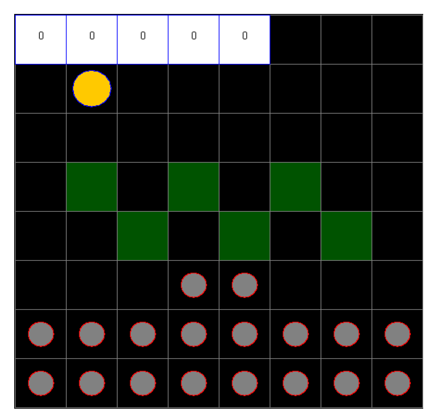
4.1. Asymmetric Adversarial Environment Modeling

Combat is a typical adversarial scenario. Real-time strategy games (RTS) face similar problems to combat (e.g., a limited decision time, huge state space, and a dynamic environment). Therefore, using RTS to study the online planning method in the asymmetric adversarial environment not only ensures the portability of the results but also reduces the research cost and improves the research efficiency.

In this work, we design an asymmetric adversarial environment based on the microRTS [21]. The microRTS offers the possibility for the agent to act as a player by providing them with information about the game state. Figure 3 illustrates a sample scenario in the asymmetric adversarial environment that will be used in our experiment. The agent controls two types of unit, the base (white square unit) and the light military unit (yellow circular unit). The opponent controls one type of unit, the worker (gray circular unit). The static obstacles are represented by green squares.

In this section, we model the online planning problem in the asymmetric adversarial environment as an MDP. The state space, action space, transition function, and reward function are defined as follows.

State space. The joint state of online planning in the asymmetric adversarial environment contains state variables that cover all units. It is represented as a high dimensional vector $s=\left(s_0,s_1,s_2,\dots s_n\right)$, which includes the information of $n$ units. For each unit, the state variable $s$ is defined as $s=\left(player,x,y,hp\right)$, where $\left(x,y\right)$ is the current position, $player$ is the owner of the unit (red or blue), and $hp$ represents the health points. The initial health points of the base, light, and worker are 10, 4, and 1, respectively.

Action space. Each movable unit has nine optional primitive actions, which are listed as follows:

• Four navigation actions: NavUp (move upward), NavDown (move downward), NavLeft (move leftward), and NavRight (move rightward).
• Four attack actions: FirUp (fire upward), FirDown (fire downward), FirLeft (fire leftward), and FirRight (fire rightward).
• Wait.

Transition function. Each move action has an 0.9 probability of moving to the target position successfully and a probability of 0.1 of staying in the current position. Each fire action has an 0.9 probability of damaging the opponent successfully, and a probability of 0.1 of failing.

Reward function. Each primitive action has a reward of −1. If the agent attacks the opponent successfully and the opponent loses 1 health point, the agent will get a reward of 20. Conversely, if the agent is attacked by the opponent and loses 1 health point, it will get a reward of −20. Moreover, the reward is 100 for winning the game and −100 for losing the game.

4.2. MAXQ Hierarchical Decomposition

In this section, we will describe the MAXQ hierarchical decomposition method over the overall task hierarchies in detail. First, we define a set of subtasks at different levels according to the related domain knowledge, which are used as the building blocks to construct the task hierarchies. Then, we extend the MDP to the SMDP by introducing hierarchical tasks and derive the MAXQ hierarchical decomposition over the defined hierarchical tasks.

The hierarchical subtasks are defined as follows:

-

NavUp, NavDown, NavLeft, NavRight, FirUp, FirDown, FirLeft, FirRight, and Wait: These actions are defined by the RTS; they are primitive actions. When a primitive action is performed, a local reward of −1 will be assigned to each primitive action. This method ensures that the online policy of the high-level subtask can reach the corresponding goal state as soon as possible.

-

NavToNeaOpp, NavToCloBaseOpp, and FireTo: The NavToNeaOpp subtask will move the light military unit to the closest enemy unit as soon as possible by performing NavUp, NavDown, NavLeft, and NavRight actions and taking into account the action uncertainties. Similarly, the NavToCloBaseOpp subtask will move the light military unit to the enemy unit closest to the base as fast as possible. The goal of the FireTo subtask is to attack enemy units within a range.

-

Attack and Defense: The purpose of Attack is to destroy the enemy’s units to win by planning the attacking behaviors, and the purpose of Defense is to defend against the enemy’s units to protect bases by carrying out defensive behaviors.

-

Root: This is a root task. The goal of Root is to destroy the enemy’s units and protect bases. In the Root task, the Attack subtask and the Defense subtask are evaluated by the hierarchical UCB1 policy according to the HMCTS-OP, which is described in the next section in detail.

The overall task hierarchies of the online planning problem in the asymmetric adversarial environment are shown in Figure 4. The parentheses after the name of a subtask indicate that the subtask has parameters.

According to the theory proposed by He et al. [3], the computational cost of action branching shrinks from $O({\left|A\right|}^T)$ to $O({\left|\tilde{A}\right|}^{T/L})$ [3] by introducing high level subtasks (macro actions), where $A$ is a set of primitive actions, $\tilde{A}$ is a set of high level subtasks, $T$ is the planning horizon, and $L\ge 1$ is an upper-bound on the length of each high-level subtask. In this work, the stochastic branching factor of the root node is reduced from 9 to 3 by introducing the MAXQ-based hierarchical subtasks. Therefore, $\left|\tilde{A}\right|=\left|A\right|/3$ and $T/L\le T$ when $L\ge 1$. As a result, the computational complexity is significantly reduced in the planning problem with a long planning horizon, which enables the algorithm to search deeper to find a better plan.

Based on the task hierarchies defined above, we extend the MDP to the SMDP by including an explicit reference to the subtasks. We introduce the variable $k$ to represent the execution time steps of the subtask.

The transition function $P:S\times A\times S\times k\to \left[0,1\right]$ represents the probability of performing subtask $a$ in state $s$ and transitioning to state $s^{\prime }$ after $k$ time steps.

$$P(s^{\prime },k|s,a)=Pr\{s_{t+k}=s^{\prime }|s_t=s,a_t=a\}.$$

(5)

The reward function of the hierarchical task accumulates the single step rewards when it is executed. The accumulation manner is related to the performance measure of HMCTS. In this work, we use the discount factor $\gamma$ to maximize the accumulated discounted rewards.

We derive the MAXQ hierarchical decomposition as follows, according to Equations (1)–(3).

$$Q(Root,s,Attack)=V(Attack,s)+{\displaystyle \sum _{s^{\prime },k}P(s^{\prime },k|s,Attack)}{\gamma }^{k}V(Root,s^{\prime })$$

(6)

$$Q(Root,s,Defense)=V(Defense,s)+{\displaystyle \sum _{s^{\prime },k}P(s^{\prime },k|s,Defense)}{\gamma }^{k}V(Root,s^{\prime })$$

(7)

$$Q(Root,s,Wait)=R(Wait,s)+{\displaystyle \sum _{s^{\prime },k}P(s^{\prime },k|s,Wait)}{\gamma }^{k}V(Root,s^{\prime })$$

(8)

$$Q(Attack,s,FireTo(p))=V(FireTo(p),s)+{\displaystyle \sum _{s^{\prime },k}P(s^{\prime },k|s,FireTo(p)){\gamma }^k}V(Attack,s^{\prime })$$

(9)

$$Q(Attack,s,NavToCloOpp)=V(NavToCloOpp,s)+{\displaystyle \sum _{s^{\prime },k}P(s^{\prime },k|s,NavToCloOpp)}{\gamma }^{k}V(Attack,s^{\prime })$$

(10)

$$\begin{array}{cc}Q(Defense,s,NavToCloBaseOpp)& =V(NavToCloBaseOpp,s)\hfill \\ & +{\displaystyle \sum _{s^{\prime },k}P(s^{\prime },k|s,NavToCloBaseOpp)}{\gamma }^{k}V(Defense,s^{\prime })\hfill \end{array}$$

(11)

$$Q(Defense,s,FireTo(p))=V(FireTo(p),s)+{\displaystyle \sum _{s^{\prime },k}P(s^{\prime },k|s,FireTo(p)){\gamma }^k}V(Defense,s^{\prime })$$

(12)

4.3. Hierarchical MCTS-Based Online Planning (HMCTS-OP)

In this section, we describe the implementation of the algorithm in detail, as shown in Algorithms 1–5. The main loop is outlined in Algorithm 1, which repeatedly invokes the execution of the HMCTS-OP function to select the optimal action (Algorithm 1, line 3). It performs this action in the current state and observes the next state (Algorithm 1 line 4) until the game terminates.

The implementation of the HMCTS-OP function is outlined in Algorithm 2. It repeatedly invokes the HMCTSimulate function within the computational budget (maximum number of iterations: 100) in the context of $\left(t,s\right)$ (Algorithm 2, line 10). Finally, it returns a greedy primitive action according to the GetGreedyPrimitive function (Algorithm 2, line 12).

The implementation of the HMCTSimulate function is outlined in Algorithm 3; this is the key component of our method. In this algorithm, each task $t$ in the MAXQ-based task hierarchies has an HMCTS-based simulation for action selection. The task $t$ could be the root task or one of the high-level subtasks or one of the primitive actions. If $t$ is a primitive action, it simulates the action in the generation model of the underlying MDP (Algorithm 3, line 4). If $t$ is a high-level subtask, there are two situations. If the node $\left(t,s\right)$ is not fully expanded, it randomly selects an untried subtask $a$ from the hierarchical subtasks of $t$ (Algorithm 3, line 16). Otherwise, it selects subtask $a$ according to the UCB sampling strategy (Algorithm 3, line 18, Equation (4)). Next, the function invokes the nested simulate process to compute the value for completing the selected subtask $a$ (Algorithm 3, line 20). Then, it computes the completion value for the end of task $t$ by the Rollout function (Algorithm 3, line 21). The value function for the MAXQ hierarchical subtask is shown in Algorithm 3 on line 22. Our algorithm is purely sample-based, so it is not necessary to estimate the transition probability of the subtask accurately. Therefore, the value function is consistent with Equations (6)–(12). Finally, the algorithm updates the node information by backpropagation (Algorithm 3, line 22–26).

The implementation of the Rollout function is outlined in Algorithm 4. It uses the hierarchical rollout policy ${\pi }_{rollout}$ (random or smart) to run the MCTS simulations. The implementation of the GetGreedyPrimitive function is outlined in Algorithm 5. It invokes the nested process to get the greedy primitive action.

Algorithm 1 PLAY.
1:	function PLAY (task $t$, state $s$, MAXQ hierarchy $M$, rollout policy ${\pi }_{rollout}$)
2:	repeat
3:	$a\leftarrow$ HMCTS-OP$\left(t,s,M,{\pi }_{rollout}\right)$
4:	$s^{\prime }\leftarrow$ Execute$\left(s,a\right)$
5:	$s\leftarrow$ s′
6:	until termination conditions
7:	end function

Algorithm 2 HMCTS-OP.
1:	function HMCTS-OP (task $t$, state $s$, MAXQ hierarchy $M$, rollout policy ${\pi }_{rollout}$)
2:	if $t$ is primitive then Return $\langle R\left(s,t\right),t\rangle$
3:	end if
4:	if $s\notin S_t$ and $s\notin G_t$ then Return $\langle -\infty ,nil\rangle$
5:	end if
6:	if $s\in G_t$ then Return $\langle 0,nil\rangle$
7:	end if
8:	Initialize search tree $T$ for task $t$
9:	while within computational budget do
10:	HMCTSSimulate ($t,s,M,0,{\pi }_{rollout}$)
11:	end while
12:	Return GetGreedyPrimitive($t,s$)
13:	end function

Algorithm 3 HMCTSSimulate.
1:	function HMCTSSimulate (task $t$, state $s$, MAXQ hierarchy $M$, depth $d$, rollout policy ${\pi }_{rollout}$)
2:	steps = 0 // the number of steps executed by task $t$
3:	if $t$ is primitive then
4:	$\left(s^{\prime },r,1\right)\leftarrow$Generative-Model$\left(s,t\right)$ // domain generative model-simulator
5:	steps = 1
6:	Return ($s^{\prime },r, steps$)
7:	end if
8:	if $t$ terminates or $d>d_{max}$ then
9:	Return ($s,0,0$)
10:	end if
11:	if node ($t,s$) is not in tree $T$ then
12:	Insert node ($t,s$) to $T$
13:	Return Rollout($t,s,d,{\pi }_{rollout}$)
14:	end if
15:	if node ($t,s$) is not fully expanded then
16:	choose $a\in$ untried subtask from $subtasks\left(t\right)$
17:	else
18:	$a=\arg ma{x}_{a^{\prime }}Q\left(t,s,a^{\prime }\right)+c\sqrt{\frac{\log N\left(t,s\right)}{N\left(t,s,a^{\prime }\right)}}$ //$a^{\prime }\in subtasks\left(t\right)$
19:	end if
20:	($s^{\prime },r,k$) = HMCTSSimulate($a,s,M,d,{\pi }_{rollout}$)
21:	($s^{″},r^{\prime },k^{\prime }$) = Rollout ($t,s^{\prime },d+k,{\pi }_{rollout}$)
22:	$r=r+{\gamma }^k{r}^{\prime }$
23:	$steps=steps+k+k^{\prime }$
24:	$N\left(t,s\right)=N\left(t,s\right)+1$
25:	$N\left(t,s,a\right)=N\left(t,s,a\right)+1$
26:	$Q\left(t,s,a\right)=Q\left(t,s,a\right)+\frac{r-Q\left(t,s,a\right)}{N\left(t,s,a\right)}$
27:	Return ($s^{″},r,steps$)
28:	end function

Algorithm 4 Rollout.
1:	function Rollout (task $t$, state $s$, depth $d$, rollout policy ${\pi }_{rollout}$)
2:	$steps=0$
3:	if $t$ is primitive then
4:	$\left(s^{\prime },r,1\right)\leftarrow$ Generative-Model$\left(s,t\right)$ // domain generative model-simulator
5:	Return ($s^{\prime },r, 1$)
6:	end if
7:	if $t$ terminates or $d>d_{max}$ then
8:	Return ($s,0,0$)
9:	end if
10:	$a~{\pi }_{rollout}\left(s,t\right)$
11:	($s^{\prime },r,k$) = Rollout($a,s,d,{\pi }_{rollout}$)
12:	($s^{″},r^{\prime },k^{\prime }$) = Rollout ($t,s^{\prime },d+k,{\pi }_{rollout}$)
13:	$r=r+{\gamma }^k{r}^{\prime }$
14:	$steps=steps+k+k^{\prime }$
15:	Return ($s^{″},r,steps$)
16:	end function

Algorithm 5 GetGreedyPrimitive.
1:	function GetGreedyPrimitive (task $t$, state $s$)
2:	if $t$ is primitive then
3:	Return $t$
4:	else
5:	$a=\arg ma{x}_{a^{\prime }}Q\left(t,s,a^{\prime }\right)$
6:	Return GetGreedyPrimitive ($a,s$)
7:	end if
8:	end function

5. Experiment and Results

5.1. Experiment Setting

Aiming to evaluate the performance of the HMCTS-OP in the asymmetric adversarial environment, we compare it with three online planning methods in three scenarios with an increasing scale, as shown in

Table 1. Details of the three scenarios used in our experiment.

	Scenario 1	Scenario 2	Scenario 3
Size	8 × 8	10 × 10	12 × 12
Units	23	23	23
Maximal states	1036	1041	1044

and Figure 5. In scenario 3, the state space contains 10⁴⁴ states, which represents a very large planning problem.

The three compared online planning methods are listed as follows:

UCT: This is a standard instance of an MCTS algorithm. UCB1 is used as the tree policy to select actions and is described in Equation (4). The parameter setting is $C=0.05$.

NaiveMCTS [21]: This uses naïve sampling in the MCTS. The parameter settings are ${\pi }_0\left({\epsilon }_0=0.4\right)$, ${\pi }_1\left({\epsilon }_1=0.33\right)$, ${\pi }_g\left({\epsilon }_g=0\right)$.

InformedNaiveMCTS [20]: This learns the probability distribution of actions in advance and incorporates the distribution into the NaiveMCTS.

The settings of our algorithms are as follows:

HMCTS-OP: This is a hierarchical MCTS-based online planning algorithm with a UCB1 policy. The parameter setting is a discount factor of $\gamma =0.99$.

The above four methods all use the random rollout policy for Monte Carlo simulations

Smart-HMCTS-OP: This is an HMCTS-OP algorithm equipped with a hand-coded rollout policy, which is named the smart rollout policy. The smart rollout policy randomly selects the action, and it is five times more likely to choose an attack action than other actions.

The maximal game length of each run is limited to 3000 decision cycles, after which the game is considered to be a tie. There are 10 decision cycles per second.

We tested the performance of all methods against two fixed opponents (UCT with random rollout policy and Random). The accumulated match results for each algorithm were counted for each scenario (win/tie/loss), and the score was calculated as the number of wins plus 0.5 times the number of ties (wins + 0.5 ties). The performance was evaluated using the average game time, the score, and the average cumulative reward. All of the results were obtained over 50 games.

5.2. Results

Figure 6 and

Table 2. The average cumulative reward over 50 games for each scenario and each algorithm against two fixed opponents (Random and UCT).

Opponent	Scenario	UCT	NaiveMCTS	Informed NaiveMCTS	HMCTS-OP	Smart-HMCTS-OP
Random	8 × 8	−38.94	−57.7	−153.56	109.94	276.34
	10 × 10	105.02	47.98	30.12	242.24	312.66
	12 × 12	−6.64	55.72	69.88	247.52	261.38
UCT	8 × 8	−929.98	−987.68	−995.06	−354.64	−288.38
	10 × 10	−694.42	−610.48	−840.8	−236.34	−95.5
	12 × 12	−653.12	−660.16	−659.54	−173.58	−89.34

show the summarized results from our experiments. The HMCTS-OP and the Smart-HMCTS-OP led to significant performance improvements compared with the other algorithms, as shown in Figure 6.

Specifically, from the perspective of average game time, as shown in Figure 6a,c,e, regardless of whether the opponent is Random or a UCT, the average game time of the HMCTS-OP and the Smart-HMCTS-OP was much shorter than that of other algorithms in all scenarios. As the opponent changed from Random to UCT, the average game time of all algorithms increased correspondingly. Moreover, the increased time of the HMCTS-OP was shorter than that of the three other algorithms in all scenarios, and the increased time of the Smart-HMCTS-OP was shorter than that of the three other algorithms in scenario 2 (10 × 10) and scenario 3 (12 × 12).

From the perspective of the score, as shown in Figure 6b,d,f, the scores of the HMCTS-OP and Smart-HMCTS-OP were higher than those of other algorithms in all scenarios. Moreover, when the opponent was UCT, the scores of HMCTS-OP and Smart-HMCTS-OP were much higher than those of the other algorithms.

Furthermore, Table 2 shows the average cumulative reward over 50 games for each scenario and each algorithm against two fixed opponents (Random and UCT). As shown in Table 2, the HMCTS-OP and Smart-HMCTS-OP outperformed the other algorithms. Next, we tested whether there is a significant performance difference between our algorithms and the other three algorithms from a statistical perspective.

We recorded all of the cumulative rewards of 50 games obtained from the evaluation of each algorithm in each scenario. These rewards were divided into 30 groups, as shown in

Table 3. Data groups.

Opponent	Scenario	UCT	NaiveMCTS	Informed NaiveMCTS	HMCTS-OP	Smart-HMCTS-OP
Random	8 × 8	$Grou{p}_{R11}$	$Grou{p}_{R12}$	$Grou{p}_{R13}$	$Grou{p}_{R14}$	$Grou{p}_{R15}$
	10 × 10	$Grou{p}_{R21}$	$Grou{p}_{R22}$	$Grou{p}_{R23}$	$Grou{p}_{R24}$	$Grou{p}_{R25}$
	12 × 12	$Grou{p}_{R31}$	$Grou{p}_{R32}$	$Grou{p}_{R33}$	$Grou{p}_{R34}$	$Grou{p}_{R35}$
UCT	8 × 8	$Grou{p}_{U11}$	$Grou{p}_{U12}$	$Grou{p}_{U13}$	$Grou{p}_{U14}$	$Grou{p}_{U15}$
	10 × 10	$Grou{p}_{U21}$	$Grou{p}_{U22}$	$Grou{p}_{U23}$	$Grou{p}_{U24}$	$Grou{p}_{U25}$
	12 × 12	$Grou{p}_{U31}$	$Grou{p}_{U32}$	$Grou{p}_{U33}$	$Grou{p}_{U34}$	$Grou{p}_{U35}$

. We performed statistical significance tests on these data. In this work, we used the Kruskal–Wallis one-way analysis of variance [22] to perform six tests among multiple groups of data (Group_R11~Group_R15, Group_U11~Group_U15, Group_R21~Group_R25, Group_U21~Group_U25, Group_R31~Group_R35, Group_U31~Group_U35) for each scenario and each opponent. Figure 7 and

Table 4. p-values of significance tests among multiple groups.

Group	GroupR11–GroupR15	GroupU11–GroupU15	GroupR21–GroupR25	GroupU21–GroupU25	GroupR31–GroupR35	GroupU31–GroupU3
p-value	1.2883 × 10−12	1.2570 × 10−32	7.5282 × 10−13	3.1371 × 10−22	3.0367 × 10−11	3.6793 × 10−22

show that there were significant differences in cumulative rewards between different algorithms for all scenarios and opponents.

Moreover, we performed multiple tests for each pair to test the following hypotheses at level ${\alpha }_0=0.05$:

$H_0$: There were no significant differences between the HMCTS-OP/Smart-HMCTS-OP and the UCT/NaiveMCTS/Informed NaiveMCTS in scenarios 1, 2, and 3 against the Random/UCT.

Our test rejected a null hypothesis if and only if the p-value was, at most, ${\alpha }_0$ [23].

Table 5. p-values of multiple tests for each pair.

Opponent	Scenario	Group	UCT	NaiveMCTS	Informed NaiveMCTS
Random	8 × 8	HMCTS-OP	0.4145	0.2623	0.0115
		Smart-HMCTS-OP	1.7033 × 10−7	4.0795 × 10−8	9.9303 × 10−9
	10 × 10	HMCTS-OP	0.1634	0.0331	0.0010
		Smart-HMCTS-OP	6.7051 × 10−7	2.6123 × 10−8	9.9410 × 10−9
	12 × 12	HMCTS-OP	6.2448 × 10−6	4.2737 × 10−4	6.7339 × 10−4
		Smart-HMCTS-OP	1.1508 × 10−7	1.4085 × 10−5	2.4075 × 10−5
UCT	8 × 8	HMCTS-OP	9.9611 × 10−9	9.9217 × 10−9	9.9217 × 10−9
		Smart-HMCTS-OP	9.9230 × 10−9	9.9217 × 10−9	9.9217 × 10−9
	10 × 10	HMCTS-OP	1.1821 × 10−6	1.9423 × 10−4	9.9353 × 10−9
		Smart-HMCTS-OP	9.9718 × 10−9	5.6171 × 10−8	9.9217 × 10−9
	12 × 12	HMCTS-OP	7.1822 × 10−8	3.0630 × 10−8	1.5334 × 10−8
		Smart-HMCTS-OP	9.9384 × 10−9	9.9260 × 10−9	9.9225 × 10−9

shows the p-values of multiple tests for each pair. Moreover, we used the Tukey–Kramer test to adjust the p-values to correct for the occurrence of false positives. As shown in Table 5, the p-values were smaller than ${\alpha }_0$ for all tests when the opponent was UCT, and the differences were significant between the Smart-HMCTS-OP and the other three algorithms for all scenarios and opponents.

Based on the experimental results, we can see that HMCTS-OP and Smart-HMCTS-OP perform significantly better than other methods. Moreover, the Smart-HMCTS-OP improves the HMCTS-OP significantly with the help of the smart rollout policy. The introduction of attack-biased rollout policies can be seen as an advantage of HMCTS-OP.

However, the drawback of HMCTS-OP is that we need to use a significant amount of domain knowledge to construct the task hierarchies, which is challenging for very complex problems. On the other hand, due to the introduction of domain knowledge, compared with other methods, the performance of the HMCTS-OP and the Smart-HMCTS-OP is greatly improved by using MAXQ-based task hierarchies to reduce the search space and guide the search process. Therefore, one of our areas of future work is to discover the underlying MAXQ-based task hierarchies automatically.

6. Conclusions

In this work, we proposed the HMCTS-OP, a novel and scalable hierarchical MCTS-based online planning method. The HMCTS-OP integrates the MAXQ-based task hierarchies and hierarchical MCTS algorithms into the online planning framework. The aim of the method is to tackle online planning with a long horizon and huge state space in the asymmetric adversarial environment. In the experiment, we empirically showed that the HMCTS-OP outperforms other methods in terms of the average cumulative reward, average game time, and accumulated score in three scenarios against Random and UCT. In the future, we plan to explore the performance of the HMCTS-OP in more complex problems. Moreover, we would like to solve the problem of automatically discovering underlying MAXQ-based task hierarchies. This is especially important for improving the performance of hierarchical learning and planning in larger, complex environments.

References

1. Vien, N.A.; Toussaint, M. Hierarchical Monte-Carlo Planning. In Proceedings of the Twenty-Ninth AAAI Conference on Artificial Intelligence, Austin, TX, USA, 25–30 January 2015; pp. 3613–3619. [Google Scholar]
2. Hostetler, J.; Fern, A.; Dietterich, T. State Aggregation in Monte Carlo Tree Search. In Proceedings of the Twenty-Eighth AAAI Conference on Artificial Intelligence, Québec City, QC, Canada, 27–31 July 2014. [Google Scholar]
3. He, R.; Brunskill, E.; Roy, N. PUMA: Planning under Uncertainty with Macro-Actions. In Proceedings of the Twenty-Fourth AAAI Conference on Artificial Intelligence, Atlanta, GA, USA, 11–15 July 2010; Volume 40, pp. 523–570. [Google Scholar]
4. Dietterich, T.G. Hierarchical Reinforcement Learning with the MAXQ Value Function Decomposition. J. Artif. Intell. Res. 2000, 13, 227–303. [Google Scholar] [CrossRef] [Green Version]
5. Puterman, M.L. Markov Decision Processes: Discrete Stochastic Dynamic Programming; John Wiley & Sons: New York, NY, USA, 1994; ISBN 0471619779. [Google Scholar]
6. Browne, C.; Powley, E. A survey of monte carlo tree search methods. IEEE Trans. Comput. Intell. AI Games 2012, 4, 1–49. [Google Scholar] [CrossRef] [Green Version]
7. Kocsis, L.; Szepesvári, C. Bandit Based Monte-Carlo Planning. In European Conference on Machine Learning; Springer: Berlin/Heidelberg, Germany, 2006; pp. 282–293. ISBN 978-3-540-45375-8. [Google Scholar]
8. Auer, P.; Cesa-Bianchi, N.; Fischer, P. Finite-time analysis of the multiarmed bandit problem. Mach. Learn. 2002, 47, 235–256. [Google Scholar] [CrossRef]
9. Sutton, R.S.; Barto, A.G. Reinforcement Learning: An Introduction, 2nd ed.; MIT Press: London, UK, 2018. [Google Scholar]
10. Črepinšek, M.; Liu, S.H.; Mernik, M. Exploration and exploitation in evolutionary algorithms: A survey. ACM Comput. Surv. 2013, 45, 1–33. [Google Scholar] [CrossRef]
11. Li, Z.; Narayan, A.; Leong, T. An Efficient Approach to Model-Based Hierarchical Reinforcement Learning. In Proceedings of the Thirty-First AAAI Conference on Artificial Intelligence, San Francisco, CA, USA, 4–10 February 2017; pp. 3583–3589. [Google Scholar]
12. Doroodgar, B.; Liu, Y.; Nejat, G. A learning-based semi-autonomous controller for robotic exploration of unknown disaster scenes while searching for victims. IEEE Trans. Cybern. 2014, 44, 2719–2732. [Google Scholar] [CrossRef] [PubMed]
13. Schwab, D.; Ray, S. Offline reinforcement learning with task hierarchies. Mach. Learn. 2017, 106, 1569–1598. [Google Scholar] [CrossRef] [Green Version]
14. Le, H.M.; Jiang, N.; Agarwal, A.; Dudík, M.; Yue, Y.; Daumé, H. Hierarchical imitation and reinforcement learning. In Proceedings of the ICML 2018: The 35th International Conference on Machine Learning, Stockholm, Sweden, 10–15 July 2018; Volume 7, pp. 4560–4573. [Google Scholar]
15. Bai, A.; Wu, F.; Chen, X. Online Planning for Large Markov Decision Processes with Hierarchical Decomposition. ACM Trans. Intell. Syst. Technol. 2015, 6, 1–28. [Google Scholar] [CrossRef]
16. Bai, A.; Srivastava, S.; Russell, S. Markovian state and action abstractions for MDPs via hierarchical MCTS. In Proceedings of the IJCAI: International Joint Conference on Artificial Intelligence, New York, NY, USA, 9–15 July 2016; pp. 3029–3037. [Google Scholar]
17. Menashe, J.; Stone, P. Monte Carlo hierarchical model learning. In Proceedings of the fourteenth International Conference on Autonomous Agents and Multiagent Systems, Istanbul, Turkey, 4–8 May 2015; Volume 2, pp. 771–779. [Google Scholar]
18. Sironi, C.F.; Liu, J.; Perez-Liebana, D.; Gaina, R.D. Self-Adaptive MCTS for General Video Game Playing Self-Adaptive MCTS for General Video Game Playing. In Proceedings of the International Conference on the Applications of Evolutionary Computation; Springer: Cham, Switzerland, 2018. [Google Scholar]
19. Neufeld, X.; Mostaghim, S.; Perez-Liebana, D. A Hybrid Planning and Execution Approach Through HTN and MCTS. In Proceedings of the IntEx Workshop at ICAPS-2019, London, UK, 23–24 October 2019; Volume 1, pp. 37–49. [Google Scholar]
20. Ontañón, S. Informed Monte Carlo Tree Search for Real-Time Strategy games. In Proceedings of the IEEE Conference on Computational Intelligence in Games CIG, New York, NY, USA, 22–25 August 2017. [Google Scholar]
21. Ontañón, S. The combinatorial Multi-armed Bandit problem and its application to real-time strategy games. In Proceedings of the Ninth Artificial Intelligence and Interactive Digital Entertainment Conference AIIDE, Boston, MA, USA, 14–15 October 2013; pp. 58–64. [Google Scholar]
22. Theodorsson-Norheim, E. Kruskal-Wallis test: BASIC computer program to perform nonparametric one-way analysis of variance and multiple comparisons on ranks of several independent samples. Comput. Methods Programs Biomed. 1986, 23, 57–62. [Google Scholar] [CrossRef]
23. Morris, H.; Degroot, M.J.S. Probability and Statistics, 4th ed.; Addison Wesley: Boston, MA, USA, 2011; ISBN 0201524880. [Google Scholar]
Figure 1. A graphic example of MAXQ-based task hierarchies.
Symmetry 12 00719 g001
Figure 2. The basic process of the Monte Carlo Tree Search (MCTS) approach.
Symmetry 12 00719 g002
Figure 3. One of the scenarios in the asymmetric adversarial environment.
Symmetry 12 00719 g003
Figure 4. The overall task hierarchies of the online planning problem in the asymmetric adversarial environment.
Symmetry 12 00719 g004
Figure 5. The three scenarios used in our experiment.
Symmetry 12 00719 g005
Figure 6. The average game time and scores of 50 games for each scenario and each algorithm against two fixed opponents (Random and UCT): (a,b) the results in scenario 1; (c,d) the results in scenario 2; (e,f) the results in scenario 3.
Symmetry 12 00719 g006aSymmetry 12 00719 g006b
Figure 7. Significance tests between algorithms for each scenario and each opponent.
Symmetry 12 00719 g007aSymmetry 12 00719 g007bSymmetry 12 00719 g007c