Deforming Gibbs Factor Using Tsallis q-Exponential with a Complex Parameter: An Ideal Bose Gas Case


Department for Theoretical Physics, Ivan Franko National University of Lviv, 12 Drahomanov St., UA-79005 Lviv, Ukraine
Symmetry 2020, 12(5), 732; https://doi.org/10.3390/sym12050732
Submission received: 29 March 2020
/
Revised: 15 April 2020
/
Accepted: 28 April 2020
/
Published: 5 May 2020
(This article belongs to the Special Issue PT-Symmetry in Physical Systems)
Abstract
:The paper presents a study of a non-standard model of fractional statistics. The exponential of the Gibbs factor in the expression for the occupation numbers of ideal bosons is substituted with the Tsallis q-exponential and the parameter is considered complex. Such an approach predicts quantum critical phenomena, which might be associated with -symmetry breaking. Thermodynamic functions are calculated for this system. Analysis is made both numerically and analytically. Singularities in the temperature dependence of fugacity and specific heat are revealed. The critical temperature is defined by non-analyticities in the expressions for the occupation numbers. Due to essentially transcendental nature of the respective equations, only numerical estimations are reported for several values of parameters. In the limit of some simplifications are obtained in equations defining the temperature dependence of fugacity and relations defining the critical temperature. Applications of the proposed model are expected in physical problems with energy dissipation and inderdisciplinarily in effective description of complex systems to describe phenomena with non-monotonic dependencies.
1. Introduction
The concept of space-time reflection symmetry commonly referred to as -symmetry (parity–time symmetry) [1] has recently entered a vast class of problems in classical and quantum physics, with both theoretical and experimental domains ranging from acoustics and mostly optics to topological insulators and metamaterials, see [2] and references therein. Being primarily associated with non-Hermitian Hamiltonians containing complex-valued potentials [3,4,5,6], -symmetry breaking in non-conservative quantum systems is linked to quantum critical phenomena of a special sort [7]. This brings a broader context to such structures as appearance of complex-valued quantities in physical problems means dissipative or decay processes, from a classical example of complex refractive index [8] (Chap. 9.4) to Bose–Einstein condensation in leaking optical lattices [9]. Applications of complex thermodynamic quantities are exemplified by temperature [10], chemical potential [11,12,13], energy [14] or magnetic field [15].
Another concept considered in the present work is nonextensive and nonadditive distributions, which originated from information theory almost sixty years ago [16,17]. They were brought into physics by Tsallis [18] and gained multidisciplinary applications in studies of complex systems in the domain of biology, climatology, economics, linguistics, and many other fields [19]. Tsallis-like generalizations are usually applied to systems with significantly pronounced non-Markovian (memory) effects [20].
Various approaches are known to nonextenside and nonadditive generalizations of quantum gases, in particular both ideal [21,22,23,24,25,26] and interacting [27] Bose gas. In the present work, the approach from paper [25] is extended to complex values of the nonextensivity parameter q in the Tsallis exponential [28]. Curiously, generalizations of the Tsallis entropy to the complex values domain were not popular until last decade [29,30,31,32,33]. Applications of the complex nonextensivity parameter include interpretation of data on high-energy particle collisions [32,34], studies of directed networks [35], analysis of complex neural networks [36], and even are related to the income distribution [37].
The paper is organized as follows. Section 2 contains basic expressions and the description of the calculation procedure. These are further detailed in Section 3. Numerical results and analytical high-temperature behavior of thermodynamic functions are presented in Section 4. Critical point is analyzed in Section 4 and some limiting analytical results are obtained in Section 6. Brief discussion in Section 7 followed by a short Materials and Methods section conclude the paper.
2. Starting Points
For the sake of completeness, let us briefly summarize the procedure to calculate thermodynamic functions, cf. [25]. Mean occupation numbers of the jth level with energy are functions of temperature T and fugacity z. Their sum over all the levels with degeneracies yields the total number of particles in the system:
Solving this equation implicit for z, one obtains . This solution has to be inserted in the definition of the total energy
leading to . Subsequent calculations are quite straightforward. For instance, specific heat, which is used in the paper to demonstrate peculiarities in the behavior of thermodynamic functions, is just
The expression for the mean occupation numbers is chosen in the following form:
where the exponential in the Gibbs factor is substituted with the so called Tsallis q-exponential [28]
This is a phenomenologically introduced generalization of the well-known expression for bosons [38] (p. 82),
and thus the model considered in the present work corresponds to a fractional quantum statistics. This notion is understood here in a wide sense, as a statistics differing from standard Bose–Einstein or Fermi–Dirac one, cf. [39]. Such types of statistics might be also referred to as “intermediate” or “exotic”.
To make a step further comparing to previous studies [25], the parameter q is considered a complex number being represented in the form
Note that complex parameters in various types of deformed statistics can be used, in particular, to effectively account for maximal level occupancy [40], interparticle interactions [41] or small dissipative branch in elementary excitation spectra [42,43].
To simplify the mathematical treatment of the problem, the summation over the levels in (1) and (2) is changed to the integration over energies with the density of states :
and
Such a change is justified primarily for interlevel separations much smaller comparing to the temperature T. Infinitely small energy level separations also appear in the thermodynamic limit: for instance, for free particles in a box with side L the quantized values of energies scale as at and for D-dimensional harmonic oscillators the frequencies scale as at .
The density of states is considered in the form [44]
where the constant A depends on parameters of the system under study, e.g., particle mass or oscillator frequency. Some particular values of s include for free particles in a D-dimensional box or for harmonic oscillators in D dimensions [45]. A more general dispersion relation , yields the dependence [39] (p. 150). The explicitly written factor of N simplifies analysis in the thermodynamic limit [44].
3. Calculations of Fugacity and Energy
The equation defining fugacity z is
For complex , the function is multivalued; the principal branch is considered in the calculations throughout this work. Making a simple change of variables , we can write two equations—separately for real and imaginary parts—as follows:
They define the temperature dependence of the complex-valued fugacity . The total energy per particle is then given by
We thus immediately see that purely imaginary parameter is not applicable. From intermediate transformations,
it becomes clear that negative values of should not be considered as well. So, after simple manipulations the relation between s and is as follows:
Moreover, one should also take into consideration that the calculation of energy requires integration [see (9) or (13)] with . Finally, we arrive at
Consider, for instance, and being one of the values attempted by the author. This yields , although satisfying the condition but making the integral for the calculation of energy very slowly convergent. To avoid such numerical issues, further in the paper the values of are chosen to ensure the right part of (17) well apart from unity.
The integrations in (12) and (13) can be carried out similarly to ordinary Bose gas problem [46] [Chap. V], by expanding the integrands into series (at least for ) [25]. The resulting expressions, e.g.,
are written using a generalization of the polylogarithm function, which is represented by the following series for
where is the beta function, and defined by the integral in (18) otherwise. In the limit of it coincides with the ordinary polylogarithm (also called Jonquière’s function or Bose–Einstein integral)
The first (integral) definition in (20) applies for all complex z except for purely real z with . The second one is valid for complex z with . Note that if the polylogarithm reduces to Riemann’s zeta function, .
Technical difficulties in solving the equation for fugacity
are caused by problems in inverting the function, as the respective analytical expressions are not even known for ordinary polylogarithms, cf. [43]. We thus will rely on numerical analysis and only obtain some limiting dependencies analytically.
4. Numerical Results and High-Temperature Behavior
In Figure 1 and Figure 2, the results of numerical calculations for fugacity and specific heat are shown for several values of and s. The units of temperature and energy are . Except for , singularities in the temperature dependencies of the fugacity are observed at certain temperatures . This critical point is discussed in more detail in the next section. For , the values of z are fixed equal to their values at the critical temperature . This is done by analogy with both ordinary ideal Bose gas and its nonadditive generalization [25], where the fugacity equals unity below the critical temperature. The low-temperature behavior is just entirely guided by the exponent s, yielding in particular the specific heat .
From Equation (11) defining fugacity, it is immediately clear that the following symmetry holds: the sign change in yields the sign change in , as one can observe in the right panel of Figure 1. Indeed, these sign changes just correspond to complex conjugation, while the right-hand side of the respective equation contains a real number N. Obviously, real part remains unchanged at .
We can see in particular that above the critical point a maximum is observed on the specific heat curve for complex-valued , but not for the real one (). A similar picture was discovered for another fractional statistics with a complex parameter [43].
At high temperatures, specific heat tends to a constant limit, which can be obtained exactly as in [25], namely:
The values of high-temperature specific heat together with critical temperatures and the respective critical fugacities are summarized in Table 1. Note that for , the expected classical value of the specific heat is recovered.
For , the zero value of the critical temperature is written formally: this means that no critical point exists for such a system. The same situation is known for the ordinary ideal Bose gas of particles in a box in two dimensions or two-dimensional harmonic oscillators, both having the density of states .
As one can see, the values of the critical temperature decrease with the imaginary part increasing. This observation correlates, in particular, with the results of [47], where the critical behavior of an interacting Bose gas in an optical lattice was studied.
5. Towards the Critical Point
The critical point is achieved when singularities occur under integrals in (12) or (13). This in turn corresponds to
Therefore, the following set of four equations
defines four variables at the critical point: being the critical temperature, the fugacity value at the critical temperature , and the coordinate where the singularity occurs.
Keeping only terms up to linear in and , we have thus
yielding two equations (for the real and imaginary parts):
From the second equation we obtain (linear in and )
The leading order of (27) defines the singular coordinate as follows:
The link between the real and imaginary parts of the fugacity is thus
Thus, the critical temperature corresponds to the point when the solutions and of first two equations in (24) satisfy relation (31). Note that the solution with should be taken, see (30).
We can now discuss what happens at temperatures below . It is worth recalling the ordinary ideal Bose gas with . From Equation (30) we obtain the singular coordinate corresponding to the ground state for all temperatures , and, consequently, a macroscopic (mathematically infinite) number of particles in the ground state,
see (6). This phenomenon is known as the Bose–Einstein condensation and is the condensate fraction. As the contribution of the single level is a macroscopic number, it is not taken into account properly when changing summation over energy levels with integration and should be written explicitly.
In the considered model with a complex q-exponential the situation is slightly different. Equation (30) means in this case that singularities occur at different energy levels at different temperatures, so that . The number of particles on these levels form an analog of the Bose condensate, with the fraction easily obtained in the following form:
The respective illustration is shown in Figure 3.
6. The Limit of
One can also perform analysis of other expressions in the limit of small . Using the series definition at given by (19), from (18) one gets:
The limiting behavior of the beta function with one parameter fixed and the other tending to infinity is [48]
This yields immediately:
Keeping only terms linear in we finally obtain:
The same equation can be derived with the integral definition (18) by expanding the Tsallis exponential into series over :
The second integral evaluates to the derivative of the polylogarithm, which can be subsequently transformed using the identity
This yields
identical to the previously obtained Equation (37) due to the well-known recursion property of the gamma function .
Let us return to Equation (37) and write polylogarithms as the series over explicitly:
Keeping only linear terms in and (which should also be small at small deviations from the real-valued statistics), we obtain for the real and imaginary parts:
so the following relation holds in the limit of :
Further analytical treatment, however, is not possible even in this limit. Series representations of polylogarithms around or involve powers of [48] and thus equations remain essentially transcendental.
7. Discussion
A new type of fractional statistics has been suggested in the paper. It pleaches the nonadditivity and complex nature of the statistics parameter, yielding thus a broader spectrum of properties. Thermodynamics of the ideal Bose gas with the Gibbs factor deformed using the Tsallis q-exponential in case of complex has been studied. The analysis has been conducted mostly numerically, with the limiting behavior for obtained analytically.
The studied system exhibits critical behavior caused by non-analyticities in the expression for occupation numbers. At the critical temperature , specific heat has a discontinuity meaning thus a second-order phase transition. The values of decrease as the power in the density of states (or space dimensionality) increase. The decrease of has been also observed for the imaginary part of the statistics parameter increasing while keeping other parameters fixed.
Analytical expressions for thermodynamic functions involve a deformed polylogarithm function . Detailed studies of its properties in the complex domain would significantly facilitate future analysis of the considered model and allow for deeper understanding of the relation between the parameter and critical behavior. This include better analytical estimations for the critical temperature and clarification of the temperature dependencies for .
Discontinuities in the specific heat at the critical temperature resemble those known for ordinary bosons, which can be caused by interparticle interactions or effective space dimensionality greater than three. The complex nature of the statistics parameter suggests that such bosonic systems with energy dissipation could be potential fields for the application of the model proposed in the present work. The respective quantum critical phenomena could be connected with the -symmetry breaking and the order parameter appearing in such problems is linked to the imaginary part of the fugacity. Finally, interdisciplinary applications of the analyzed statistics is envisaged for phenomena with non-monotonic dependencies, which is related to the complex parameter in the expression for occupation numbers.
8. Materials and Methods
Numerical computations in the work are made in wxMaxima 13.04.2, a graphical interface for the computer algebra system MAXIMA (http://maxima.sourceforge.net). In particular, integrations are carried out by the Quadpack function quad_qagi, see https://web.csulb.edu/~woollett/mbe8nint.pdf. Numerical equation solutions are obtained by the mnewton procedure from the mnewton package (https://web.csulb.edu/~woollett/mbe4solve.pdf).
Funding
This research was partly funded by the Ministry of Education and Science of Ukraine, grant number 0119U002203.
Acknowledgments
I am grateful to the anonymous referees for their comments and suggestions, which helped me to extend the manuscript.
Conflicts of Interest
The author declares no conflict of interest.
References
- Bender, C.M.; Boettcher, S. Real spectra in non-Hermitian Hamiltonians having PT symmetry. Phys. Rev. Lett. 1998, 80, 5243–5246. [Google Scholar] [CrossRef] [Green Version]
- Bender, C.M.; Dorey, P.E.; Dunning, C.; Fring, A.; Hook, D.W.; Jones, H.F.; Kuzhel, S.; Lévai, G.; Tateo, R. PT Symmetry In Quantum and Classical Physics; World Scientific: Singapore, 2019. [Google Scholar] [CrossRef]
- Tkachuk, V.M.; Fityo, T.V. Factorization and superpotential of the PT symmetric Hamiltonian. J. Phys. A Math. Gen. 2001, 34, 8673–8677. [Google Scholar] [CrossRef] [Green Version]
- Guo, A.; Salamo, G.J.; Duchesne, D.; Morandotti, R.; Volatier-Ravat, M.; Aimez, V.; Siviloglou, G.A.; Christodoulides, D.N. Observation of PT-symmetry breaking in complex optical potentials. Phys. Rev. Lett. 2009, 103, 093902. [Google Scholar] [CrossRef] [PubMed] [Green Version]
- Hayward, R.; Biancalana, F. Complex Berry phase dynamics in PT-symmetric coupled waveguides. Phys. Rev. A 2018, 98. [Google Scholar] [CrossRef] [Green Version]
- El-Ganainy, R.; Makris, K.G.; Khajavikhan, M.; Musslimani, Z.H.; Rotter, S.; Christodoulides, D.N. Non-Hermitian physics and PT symmetry. Nat. Phys. 2018, 14, 11–19. [Google Scholar] [CrossRef]
- Ashida, Y.; Furukawa, S.; Ueda, M. Parity-time-symmetric quantum critical phenomena. Nat. Commun. 2017, 8. [Google Scholar] [CrossRef]
- Griffiths, D.J. Introduction to Electrodynamics, 3rd ed.; Prentice Hall: Upper Saddle River, NJ, USA, 1999. [Google Scholar]
- Ng, G.S.; Hennig, H.; Fleischmann, R.; Kottos, T.; Geisel, T. Avalanches of Bose–Einstein condensates in leaking optical lattices. New J. Phys. 2009, 11, 073045. [Google Scholar] [CrossRef]
- Matveev, V.; Shrock, R. Complex-temperature properties of the Ising model on 2D heteropolygonal lattices. J. Phys. A Math. Gen. 1995, 28, 5235–5256. [Google Scholar] [CrossRef] [Green Version]
- Chakraborty, P.K.; Nag, B.; Ghatak, K.P. On the electron energy spectrum in heavily doped non-parabolic semiconductors. J. Phys. Chem. Solids 2003, 64, 2191–2197. [Google Scholar] [CrossRef]
- Cragg, G.E.; Kerman, A.K. Complex Chemical Potential: Signature of Decay in a Bose-Einstein Condensate. Phys. Rev. Lett. 2005, 94, 190402. [Google Scholar] [CrossRef] [Green Version]
- Ipsen, J.R.; Splittorff, K. Baryon number Dirac spectrum in QCD. Phys. Rev. D 2012, 86, 014508. [Google Scholar] [CrossRef] [Green Version]
- Bender, C.M.; Brody, D.C.; Hook, D.W. Quantum effects in classical systems having complex energy. J. Phys. A Math. Theor. 2008, 41, 352003. [Google Scholar] [CrossRef] [Green Version]
- Kuzmak, A.R.; Tkachuk, V.M. Detecting the Lee-Yang zeros of a high-spin system by the evolution of probe spin. EPL (Europhys. Lett.) 2019, 125, 10004. [Google Scholar] [CrossRef]
- Rényi, A. On measures of entropy and information. In Proceedings of the 4th Berkeley Symposium on Mathematics, Statistics and Probability 1960; University of California Press: Berkeley, CA, USA, 1961; pp. 547–561. [Google Scholar]
- Daróczy, Z. Generalized information functions. Inf. Control 1970, 16, 36–51. [Google Scholar] [CrossRef] [Green Version]
- Tsallis, C. Possible generalization of Boltzmann-Gibbs statistics. J. Stat. Phys. 1988, 52, 479–486. [Google Scholar] [CrossRef]
- Gell-Mann, M.; Tsallis, C. (Eds.) Nonextensive Entropy: Interdisciplinary Applications; Oxford University Press: New York, NY, USA, 2004. [Google Scholar]
- Abe, S.; Okamoto, Y. (Eds.) Nonextensive Statistical Mechanics and Its Applications; Springer: Berlin, Germany, 2001. [Google Scholar] [CrossRef]
- Büyükkılıç, F.; Demirhan, D.; Güleç, A. A statistical mechanical approach to generalized statistics of quantum and classical gases. Phys. Lett. A 1995, 197, 209–220. [Google Scholar] [CrossRef]
- Aragão-Rêgo, H.H.; Soares, D.J.; Lucena, L.S.; da Silva, L.R.; Lenzi, E.K.; Fa, K.S. Bose–Einstein and Fermi–Dirac distributions in nonextensive Tsallis statistics: An exact study. Phys. A Stat. Mech. Appl. 2003, 317, 199–208. [Google Scholar] [CrossRef]
- Ou, C.; Chen, J. Thermostatistic properties of a q-generalized Bose system trapped in an n-dimensional harmonic oscillator potential. Phys. Rev. E 2003, 68, 026123. [Google Scholar] [CrossRef]
- Mohammadzadeh, H.; Adli, F.; Nouri, S. Perturbative thermodynamic geometry of nonextensive ideal classical, Bose, and Fermi gases. Phys. Rev. E 2016, 94, 062118. [Google Scholar] [CrossRef] [Green Version]
- Rovenchak, A. Ideal Bose-gas in nonadditive statistics. Low Temp. Phys. 2018, 44, 1025–1031. [Google Scholar] [CrossRef]
- Adli, F.; Mohammadzadeh, H.; Najafi, M.N.; Ebadi, Z. Condensation of nonextensive ideal Bose gas and critical exponents. Phys. A Stat. Mech. Appl. 2019, 521, 773–780. [Google Scholar] [CrossRef]
- Tanatar, B. Trapped interacting Bose gas in nonextensive statistical mechanics. Phys. Rev. E 2002, 65, 046105. [Google Scholar] [CrossRef] [PubMed]
- Tsallis, C. What are the numbers that experiments provide? Química Nova 1994, 17, 468–471. [Google Scholar]
- Gliozzi, F.; Tagliacozzo, L. Entanglement entropy and the complex plane of replicas. J. Stat. Mech. Theory Exp. 2010, 2010, P01002. [Google Scholar] [CrossRef] [Green Version]
- Plastino, A.; Rocca, M.C. A direct proof of Jauregui-Tsallis’ conjecture. J. Math. Phys. 2011, 52, 103503. [Google Scholar] [CrossRef] [Green Version]
- Plastino, A.; Rocca, M.C. Inversion of Umarov–Tsallis–Steinberg’s q-Fourier transform and the complex-plane generalization. Phys. A Stat. Mech. Appl. 2012, 391, 4740–4747. [Google Scholar] [CrossRef] [Green Version]
- Wilk, G.; Włodarczyk, Z. Tsallis distribution with complex nonextensivity parameter q. Phys. A Stat. Mech. Appl. 2014, 413, 53–58. [Google Scholar] [CrossRef] [Green Version]
- Matsuzoe, H.; Wada, T. Deformed algebras and generalizations of independence on deformed exponential families. Entropy 2015, 17, 5729–5751. [Google Scholar] [CrossRef] [Green Version]
- Wilk, G.; Włodarczyk, Z. Tsallis distribution decorated with log-periodic oscillation. Entropy 2015, 17, 384–400. [Google Scholar] [CrossRef] [Green Version]
- Rotundo, G.; Ausloos, M. Complex-valued information entropy measure for networks with directed links (digraphs). Application to citations by community agents with opposite opinions. Eur. Phys. J. B 2013, 86. [Google Scholar] [CrossRef]
- Ibrahim, R.; Darus, M. Analytic study of complex fractional Tsallis’ entropy with applications in CNNs. Entropy 2018, 20, 722. [Google Scholar] [CrossRef] [Green Version]
- Abreu, E.M.C.; Moura, N.J.; Soares, A.D.; Ribeiro, M.B. Oscillations in the Tsallis income distribution. Phys. A Stat. Mech. Appl. 2019, 533, 121967. [Google Scholar] [CrossRef]
- Isihara, A. Statistical Physics; Academic Press: New York, NY, USA; London, UK, 1971. [Google Scholar]
- Khare, A. Fractional Statistics and Quantum Theory, 2nd ed.; World Scientific: Singapore, 2005. [Google Scholar]
- Yang, Y.; Xie, S.; Feng, W.; Wu, X. Statistics for q-commutator in the case of qs+1 = 1. Mod. Phys. Lett. A 1998, 13, 879–886. [Google Scholar] [CrossRef]
- Gavrilik, A.M.; Rebesh, A.P. Deformed gas of p, q-bosons: Virial expansion and virial coefficients. Mod. Phys. Lett. B 2012, 25, 1150030. [Google Scholar] [CrossRef] [Green Version]
- Rovenchak, A. Phase transition in a system of 1D harmonic oscillators obeying Polychronakos statistics with a complex parameter. Low Temp. Phys. 2013, 39, 888–892. [Google Scholar] [CrossRef] [Green Version]
- Rovenchak, A. Complex-valued fractional statistics for D-dimensional harmonic oscillators. Phys. Lett. A 2014, 378, 100–108. [Google Scholar] [CrossRef]
- Rovenchak, A.; Sobko, B. Fugacity versus chemical potential in nonadditive generalizations of the ideal Fermi-gas. Phys. A Stat. Mech. Appl. 2019, 534, 122098. [Google Scholar] [CrossRef] [Green Version]
- Salasnich, L. BEC in nonextensive statistical mechanics. Int. J. Mod. Phys. B 2000, 14, 405–409. [Google Scholar] [CrossRef] [Green Version]
- Landau, L.D.; Lifshitz, E.M. Statisticsl Physics. Part 1, 3rd ed.; Pergamon Press: Oxford, UK, 1980. [Google Scholar]
- Ashida, Y.; Furukawa, S.; Ueda, M. Quantum critical behavior influenced by measurement backaction in ultracold gases. Phys. Rev. A 2016, 94, 053615. [Google Scholar] [CrossRef] [Green Version]
- The Mathematical Functions Site, 1998–2020. Available online: http://functions.wolfram.com (accessed on 20 March 2020).
Figure 1.
Fugacity for different values of s and (with the real part fixed as ). (left) Real part . (right) Imaginary part .
Figure 1.
Fugacity for different values of s and (with the real part fixed as ). (left) Real part . (right) Imaginary part .
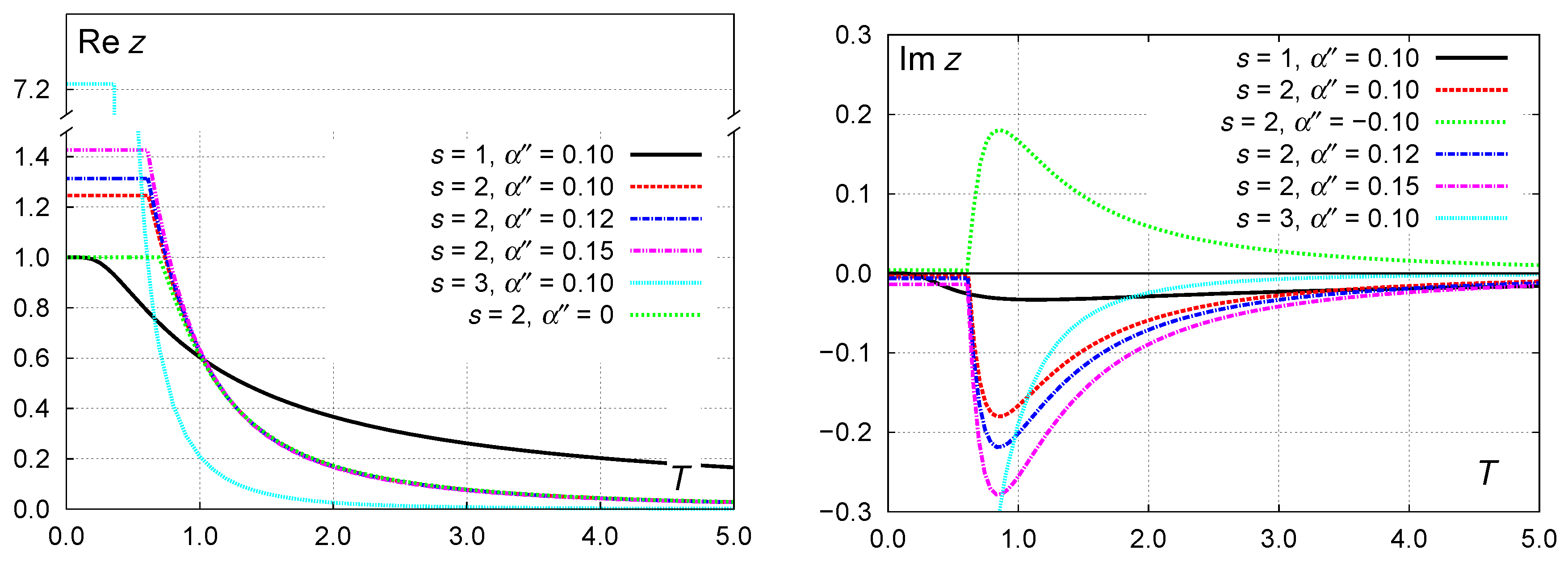
Figure 2.
Specific heat for different values of s and (with the real part fixed as ). (left) Real part . (right) Imaginary part .
Figure 2.
Specific heat for different values of s and (with the real part fixed as ). (left) Real part . (right) Imaginary part .

Figure 3.
Temperature dependence of the “condensate” fraction for and .


Table 1.
Some parameters of the ideal Bose gas deformed with a complex-valued Tsallis exponential.
| s, | at | ||
|---|---|---|---|
| , | 0 | 1 | |
| , | 0.690 | 1 | 2.857 |
| , | 0.616 | ||
| , | 0.612 | ||
| , | 0.609 | ||
| , | 0.359 |
© 2020 by the author. Licensee MDPI, Basel, Switzerland. This article is an open access article distributed under the terms and conditions of the Creative Commons Attribution (CC BY) license (http://creativecommons.org/licenses/by/4.0/).
Share and Cite
MDPI and ACS Style
Rovenchak, A. Deforming Gibbs Factor Using Tsallis q-Exponential with a Complex Parameter: An Ideal Bose Gas Case. Symmetry 2020, 12, 732. https://doi.org/10.3390/sym12050732
AMA Style
Rovenchak A. Deforming Gibbs Factor Using Tsallis q-Exponential with a Complex Parameter: An Ideal Bose Gas Case. Symmetry. 2020; 12(5):732. https://doi.org/10.3390/sym12050732
Chicago/Turabian StyleRovenchak, Andrij. 2020. "Deforming Gibbs Factor Using Tsallis q-Exponential with a Complex Parameter: An Ideal Bose Gas Case" Symmetry 12, no. 5: 732. https://doi.org/10.3390/sym12050732
Note that from the first issue of 2016, this journal uses article numbers instead of page numbers. See further details here.