Compressive Sensing Based Three-Dimensional Imaging Method with Electro-Optic Modulation for Nonscanning Laser Radar

Abstract

Low-cost Laser Detection and Ranging (LiDAR) is crucial to three-dimensional (3D) imaging in applications such as remote sensing, target detection, and machine vision. In conventional nonscanning time-of-flight (TOF) LiDAR, the intensity map is obtained by a detector array and the depth map is measured in the time domain which requires costly sensors and short laser pulses. To overcome such limitations, this paper presents a nonscanning 3D laser imaging method that combines compressive sensing (CS) techniques and electro-optic modulation. In this novel scheme, electro-optic modulation is applied to map the range information into the intensity of echo pulses symmetrically and the measurements of pattern projection with symmetrical structure are received by the low bandwidth detector. The 3D imaging can be extracted from two gain modulated images that are recovered by solving underdetermined inverse problems. An integrated regularization model is proposed for the recovery problems and the minimization functional model is solved by a proposed algorithm applying the alternating direction method of multiplier (ADMM) technique. The simulation results on various subrates for 3D imaging indicate that our proposed method is feasible and achieves performance improvement over conventional methods in systems with hardware limitations. This novel method will be highly valuable for practical applications with advantages of low cost and flexible structure at wavelengths beyond visible spectrum.

1. Introduction

Laser Detection and Ranging (LiDAR) is a remote sensing technology that obtains intensity and range of objects by transmitting laser pulses and receiving return pulses [1]. As it displays advantages of high-reliability, longitudinal resolution, and anti-electric magnetic interference ability, LiDAR is widely used in multiple areas such as target detection and recognition, remote sensing, and three-dimensional (3D) scene imaging [2,3], wherein nonscanning LiDAR system is undergoing major development in recent years because of features such as low requirement of light source, ability to detect moving objects, and image obscuring objects [4,5,6].

At present, an important experimental-research branch of 3D LiDAR system is achieving single-pixel nonscanning imaging and most of this research are based on the new sensing modality called compressive sensing (CS) [7,8,9]. This new mathematical theory was proposed by Donoho and Candès [10,11] initially and has expanded greatly since then. The CS framework for the signal acquisition was a major breakthrough in signal processing community after the famous Shannon sampling theorem. It tried to sense enough information of a sparse signal by projecting the data in a space incoherent with the data’s structure, so that the original signal can be reconstructed perfectly [12,13]. Thanks to the effort of Duarte and Davenport [14] who presented a single-pixel CS camera architecture, CS theory has expanded greatly from methodology to practice in both active and passive imaging technologies. Duarte and Davenport’s work paved the way for various succeeding 3D LiDAR applications such as Howland experimentally demonstrating a photon-counting single-pixel time-of-flight (CS-TOF) laser radar camera [15] and Sun showing a modified TOF 3D imaging system (M-CS-TOF) with an accuracy of ∼3 mm [16].

TOF imaging is performed by correlating the detection time of the back-scattered light with the time of illumination pulses [17]. As a direct ranging method, TOF imaging system depends on narrow bandwidth of illumination laser pulses and the short rise time of detectors to achieve a high range resolution. To overcome such limitations, indirect methods including time slicing (TS), intensity correlation and gain modulation in range-gated imaging systems have become increasingly popular [18,19,20]. The TS technique obtains a full depth map by recording multiple frames whose number is proportional to the required depth resolution [21]. Therefore, tons of 2D images are required to construct one 3D image with high resolution. As to intensity correlation, the range information can be restored by analyzing the intensity variation in the overlapping areas of two range-gates with a small number of distinct images [19]. However, rectangular-shaped or triangular-shaped pulses with high quality are required [22]. Furthermore, the gate widths should be carefully designed in order to adapt to the laser pulse widths [23]. On the contrary, gain modulation method is a pulse-shape-free method. It only needs two gain-modulated images to construct time-resolved imaging, making it possible to achieve accurate imaging reconstruction with less data and low-cost system [24].

In this paper, a CS-based electro-optic modulation scheme in nonscanning LiDAR and a 3D reconstruction method are proposed. This scheme combines the CS technology with gain modulation to achieve the 3D imaging of the target. Laser pulses are emitted toward the target and then the scattered light from the target returns to the system. Peak values are recorded out of total echo pulses which is the sum of echo pulses after spatial modulation and gain modulation are applied in a symmetrical procedure. Next, two modulated images can be recovered by the peak values in the CS framework corresponding to different gain modulation functions respectively. Furthermore, an intensity map and a depth map of the target scene are able to be extracted from the two recovered images which are obtained by solving underdetermined inverse problems. We propose an integrated regularization model for the recovery problems and this minimization functional model is solved by a proposed algorithm applying the alternating direction method of multiplier (ADMM) technique. As an extension of our previous related work [25], the novel resolution to the 3D imaging problem lies in the proposed method that can overcome hardware limitations, by modulating the range information into the reflective light intensity before compressive sampling. Numerical simulations for 3D imaging with various subrates are presented to demonstrate the improved performance of the proposed method.

This paper is organized as follows. Section 2 presents a prototype of the CS-based RGI system applied the electro-optic modulation method for 3D imaging and its mathematical model. Section 3 presents the 3D measurement and reconstruction using CS-based electro-optic modulation method after we review the CS theory. Section 4 shows simulation experiments based on typical discrete and continuous targets to validate the proposed method. Finally, Section 5 presents the conclusion.

2. System Description

In this section, we propose a 3D LiDAR system to implement the CS-based electro-optic modulation method. In addition, the working mechanism of the system is presented by introducing the proposed system setup and its laser pulse model.

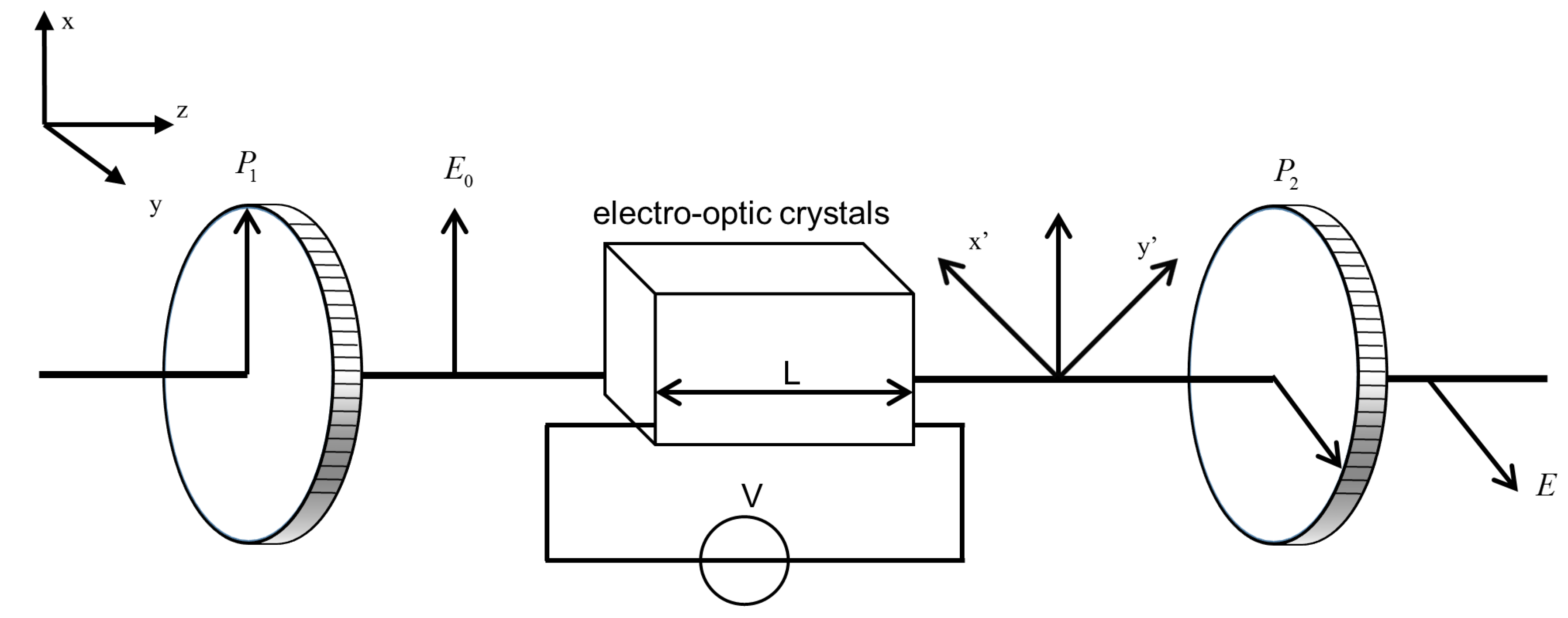
2.1. Proposed System Setup

As is shown in Figure 1, the proposed CS range-gated imaging (RGI) system mainly consists of a transmitter, a receiver, a narrowband filter (NBF), an electro-optic modulator (EOM), two polarizers, a digital micromirror device (DMD), and a one-pixel avalanche photodiode (APD) detector. There is a red light path with white arrows and blue data path in dotted line in Figure 1.

First, a pulsed laser is emitted toward the target scene. Second, reflected light returns to the RGI system. With closing the receiver’s gate while the pulsed laser is traveling, the system’s Signal-to-Noise Ratio (SNR) can be improved. Third, an EOM is used to conduct gain modulation and a DMD is applied to conduct spatial modulation with the gate open [26,27,28]. Forth, a NBF is used to remove background radiation from sunlight and other sources. Finally, the reflected light arrives at a one-pixel APD detector.

Figure 2 contains a sequence chart for the RGI system and gain modulation function. In Figure 2a, $V_{in}\left(t\right)$ and $V_{de}\left(t\right)$ are the applied voltages of the EOM to generate different gain modulations. The index “in” is short for increasing and the index “de” is short for decreasing. The intensities of the passing light are modulated with $g_{in}\left(t\right)$ and $g_{de}\left(t\right)$, respectively. Here, we define $R_0$ is the range according to the optical gate open beginning time; D with subscript is the range between the object and $R_0$ in Figure 2b,c. R is the range between the RGI system and the object; and L is the gate opening range. The laser pulse is emitted at the time of $T_0$. The gate opens at the time of $T_1$ and the opening time of RGI system is determined by the duration time of gate opening, $T_G$. According to the round-trip travel range, L is given by

$$L=\frac{1}{2}c{T}_G,$$

(1)

where c is the speed of light. Then, we can get

$$R=R_0+D.$$

(2)

The pulse received by the APD is a sum of overlapped pulses with particular modulation from different distances. Figure 2b,c explain how the components of the pulse of APD are modulated and work together. The pulses in black dash line are echo pulses from objects at different distances and they overlap with each other that results in the pulse of APD, $p_t\left(t\right)$, in black full lines. The red dash lines are gain modulation functions $g_{in}\left(t\right)$ and $g_{de}\left(t\right)$ when the gate opens, respectively. Then, the range D and R are able to be resolved from two intensity-modulated CS-based recovered images which will be introduced in detail later. Ultimately, time-resolved imaging can be achieved.

2.2. Proposed System Model

To be more specific, the system model is presented as follows. The time propagation of the laser pulse from the transmitter $p_t$ is of the form:

$$p_t\left(t\right)=\left\{\begin{array}{cc}{(t/\tau )}^2{e}^{\left(-\frac{t}{\tau }\right)}\hfill & t\ge 0\hfill \\ 0\hfill & t<0\hfill \end{array}\right.$$

(3)

where $\tau =T_{1/2}/3.5$ and $T_{1/2}$ is the full width at half maximum (FWHM) of the pulse [3]. Assuming that the target is a Lambert diffuse point-like reflector, the energy of the echo signal $E_r$ can be represented as the following formula:

$$E_r=\frac{\rho D_r^2{T}_a^2\eta }{4R^4}{\int }_{T_G}{p}_t\left(t-2R/c\right)dt,$$

(4)

where $\rho$ is the reflectance of the target, $D_r$ is the diameter of the receiver, $T_a$ is the single-pass atmospheric transmittance, $\eta$ is the efficiencies of the optical transmitting and receiving systems and R is the range between the target and the receiver [29]. Since the APD can only obtain the intensity of the pulses rather than their flying time, gain modulation by an EOM based on the electro-optic effect of crystals is applied to realize time-resolved imaging.

Figure 3 presents a typical structure of longitudinal electro-optic modulation using Pockels effect. It mainly consists of the electro-optic crystals and the polarizers, $P_1$ and $P_2$, in a universal coordinate system with x-axis, y-axis and z-axis. The polarizers are fixed and perpendicular to each other. The polarized light whose vibration is parallel to x axis enters the EOM and it is resolved into two components parallel to $x^{\prime }$ axis and $y^{\prime }$ axis respectively. When a voltage is applied to the EOM in the direction of propagation (z axis), phase retardation of the light will take place between the two components and the intensity of the light is modulated. The phase shift $\theta$ proportional to the applied voltage $V\left(t\right)$ can be given by

$$\theta =\frac{2\pi }{\lambda }{n}_0^3{\gamma }_{63}V\left(t\right),$$

(5)

where $\lambda$ is the wavelength of light, $n_0$ is the ordinary refractive indices of crystal and ${\gamma }_{63}$ is the crystal electro-optic coefficient [24]. The applied voltages are given in the monotonously increasing and decreasing form of:

$$\begin{array}{c}{V}_{in}\left(t\right)=\frac{V_{\pi }}{T_G}t,\left(0\le t\le T_G\right)\hfill \\ V_{de}\left(t\right)=V_{\pi }-\frac{V_{\pi }}{T_G}t,\left(0\le t\le T_G\right)\hfill \end{array},$$

(6)

where the half-wave voltage $V_{\pi }\left(\theta =\pi \right)$ is given by

$$V_{\pi }=\frac{\lambda }{2n_0^3{\gamma }_{63}}.$$

(7)

Then we can have the phase shift $\theta$ as a function of time t:

$$\theta =\pi ·\frac{t}{T_G},\left(0\le t\le T_G\right).$$

(8)

Applying Equation (1) to Equation (8), the function of the phase shift $\theta$ and the depth D are obtained as:

$$\theta =\pi ·\frac{D}{L},\left(0\le D\le L\right).$$

(9)

During the gated opening time, the applied voltages are $V_{in}\left(t\right)$ and $V_{de}\left(t\right)$. The intensities of the light, $E_{in}$ and $E_{de}$, are modulated with gain functions $g_{in}\left(t\right)$ and $g_{de}\left(t\right)$ respectively:

$$\begin{array}{c}{E}_{in}=E_r{sin}^2(\theta /2)\hfill \\ E_{de}=E_r{cos}^2(\theta /2)\hfill \end{array}.$$

(10)

3. CS-Based Electro-Optic Modulation Method for 3D Imaging

3.1. Compressive Sensing Theory

Compressive sensing is different from the traditional approach to digital data acquisition that samples an analog signal uniformly at or above the Nyquist rate. CS is a measurement technique to employ optimization to detect a sparse n-dimensional signal with $m<n$ samples [30].

The detection and reconstruction process can be modeled by vectors and matrices as follows. For convenience sake, we use n-dimensional vector x represents the gray value of an original image. In addition, we then take advantage of transform coding to represent the image in terms of the coefficients $\left\{{\alpha }_i\right\}$ of an orthonormal basis expansion:

$$x={\sum }_{i=1}^n{\alpha }_i{\psi }_i,$$

(11)

where ${\left\{{\psi }_i\right\}}_{i=1}^n$ are the $n\times 1$ basis vectors. We can concisely write the original image as

$$x=\Psi \alpha ,$$

(12)

by forming the coefficient vector $\alpha$ and the $n\times n$ transforming matrix $\Psi$ which is the stack of vectors ${\left\{{\psi }_i\right\}}_{i=1}^n$ as columns. For natural images, x is mostly compactly represented by considering only significant elements in the sparse basis, such as discrete cosine transform (DCT) and wavelet transform (DWT) [31,32].

In addition, we then construct a $m\ll n$ dimensional measurement vector y by multiplying x by an $m\times n$ matrix $\Phi$ describing the measurement matrix:

$$y=\Phi x+\epsilon =A\alpha +\epsilon ,$$

(13)

where vector $\epsilon$ is the additional noise. As $m\ll n$, the dimension of the signal has been reduced. Matrix A is called sensing matrix and determined by $A=\Phi \Psi$. The subsampling rate is defined by $subrate=m/n$ and conventional recover methods are incapable since $subrate<1$.

Previous research has shown that the sensing matrix obeys the so-called restricted isometry property (RIP) when $\Phi$ is drawn randomly from a suitable distribution [33]. In this way, the inverse problem of constructing the signal x from the measurements y can be achieved by solving a 1-norm ($p=1$) or 2-norm ($p=2$) minimization problem with relaxed constraints:

$$\underset{\alpha \in {\mathbb{R}}^n}{min}{\left|\right|\alpha \left|\right|}_p,s.t.\left|\right|A\alpha -{y\left|\right|}_2\le \epsilon ,$$

(14)

where $\epsilon$ bounds the amount of noise in the sampling [34]. Equation (14) is a convex problem and can be solved efficiently by various construction algorithms such as the Total Variation (TV) minimization based on augmented Lagrangian and alternating direction algorithm (TVAL3) which are able to handle different boundary conditions for $\alpha$ and widely used in CS systems [35].

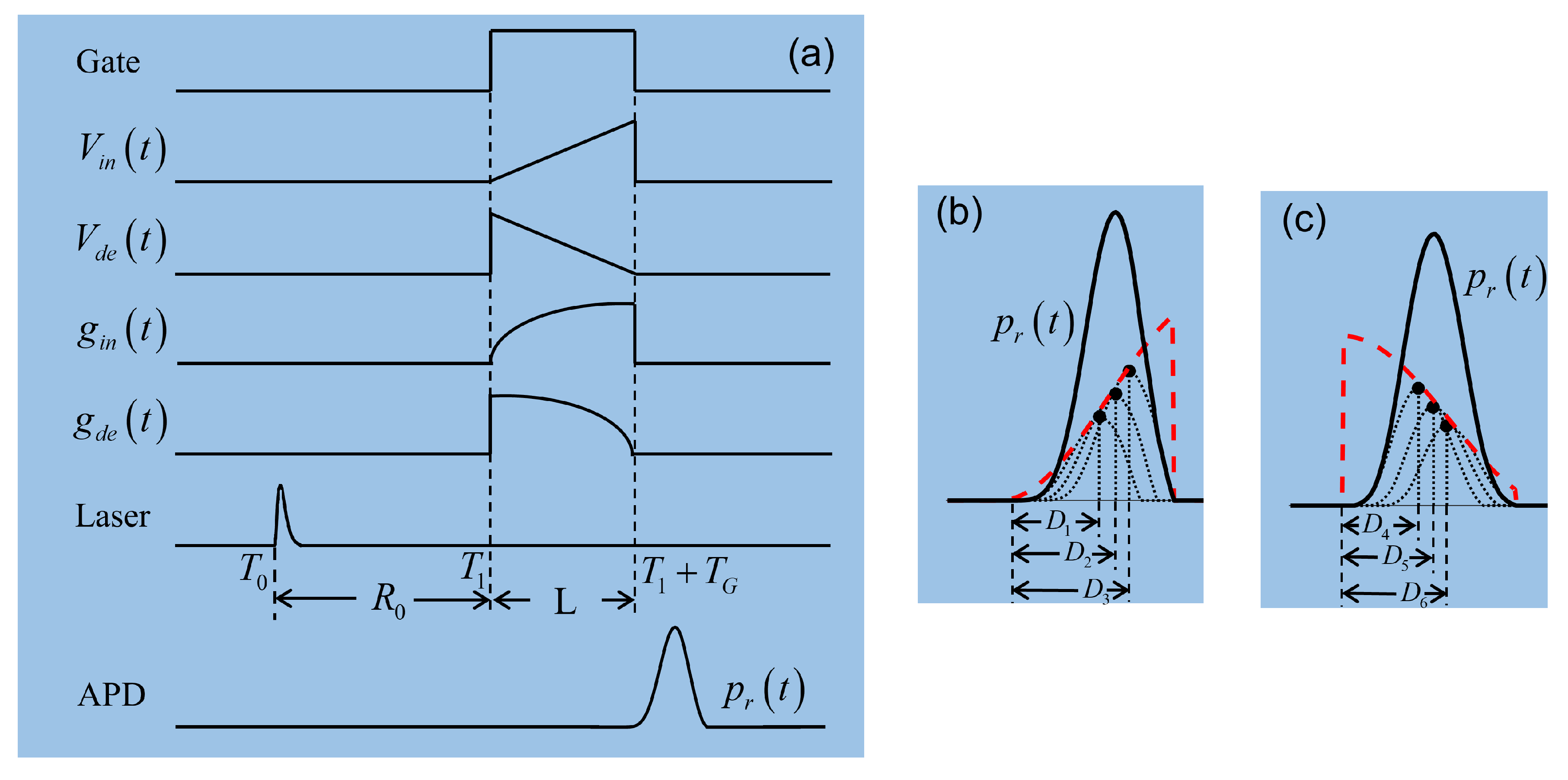
3.2. Peak Value Obtained for 3D Reconstruction

Assuming the power of the echo signal is $P_r$, the range-discretized form of the total power of echo pulses by sparse sampling in the view of field can be described as a sum of the pulses from each pixel with different amplitudes and delay times:

$$p_{r,j}\left(t\right)=\sum _{i=1}^n{\Phi }_{\left(j,i\right)}g\left(t\right)P_r\left(R_i\right)p\left(t-t_i\right),$$

(15)

where $\Phi$ is a $m\times n$ measurement matrix, $t_i=2R_i/c$ and $g\left(t\right)$ is the gain modulation function applied by the EOM.

For 3D compressive imaging, a 2D extended mathematical model of measuring process is presented as follows according to Equations (13) and (15) in a discretized matrix form:

$$Y=\Phi X{F}_{gain}+{\epsilon }_M,$$

(16)

where Y is a $m\times l$ matrix as total echo waveform, X is a $n\times l$ matrix as echo waveform from n pixels of the target scene, $F_{gain}$ is a $l\times l$ diagonal matrix as the gain modulation function and ${\epsilon }_M$ is the additive noise matrix. Only peak values of the total echo waveform are recorded as the compressive measurements rather than recording the whole waveform. In this instance, we define vector $y={\left(y_1,y_2,\cdots y_m\right)}^T$ as the CS measurements in the form of:

$$y=\Phi x_g+\epsilon =\Phi Gx+\epsilon ,$$

(17)

where $x_g={\left(x_{g,1},x_{g,2},\cdots ,x_{g,n}\right)}^T$ is the $n\times 1$ vector used to present the modulated intensity map and $\epsilon$ is the additive noise vector. $x_g$ can be presented as the product of the gain value matrix $G=diag\left(g_1,g_2,\cdots ,g_n\right)$ where $diag(·)$ represents a diagonal matrix and the $n\times 1$ vector x which presents the original echo energy from the target. Applying different voltages, $V_{in}\left(t\right)$ and $V_{de}\left(t\right)$, to the EOM, the original intensity map are modulated to $x_{in}$ and $x_{de}$. Then two sets of measurements $y_{in}$ and $y_{de}$ are achieved in the CS framework shown in Equation (17), respectively.

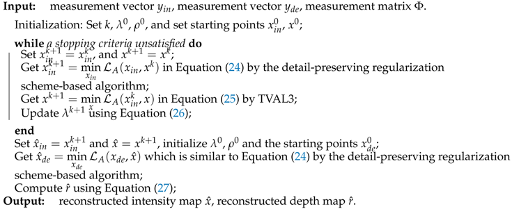
3.3. 3D Image Reconstruction

In this section, we proposed a recovery method to achieve the goal of 3D imaging according to the CS measurements $y_{in}$ and $y_{de}$. A set of inverse problem formulations within the CS framework are presented and the alternating direction method of multipliers (ADMM) combined with convex optimization algorithms is employed. In this way, the modulated intensity images are obtained to determine a range value and a gray value for each pixel in the target scene, namely $\widehat{x}={(\widehat{x_1},\widehat{x_2},\cdots ,\widehat{x_n})}^T$ and $\widehat{r}={(\widehat{r_1},\widehat{r_2},\cdots ,\widehat{r_n})}^T$, respectively.

For clarity, we present the electro-optical modulated CS measurement vectors in the form of Equation (17):

$$\begin{array}{cc}\hfill & y_{in}=\Phi x_{in}+{\epsilon }_{in}=\Phi G_{in}x+{\epsilon }_{in}\hfill \end{array}$$

(18)

$$\begin{array}{cc}\hfill & y_{de}=\Phi x_{de}+{\epsilon }_{de}=\Phi G_{de}x+{\epsilon }_{in}.\hfill \end{array}$$

(19)

There is a useful property of the gain functions for one particular target according to the proposed system model in Section 2.2, especially Equation (10). The property shows that the sum of the two gain value matrices is not only certain but also known:

$$G_{in}+G_{de}=I,$$

(20)

where I is the unit matrix.

We enforce the sparsity of the signal to be constructed in some transform domain as a prior and construct the inverse problem generally. However, reconstructions based on primary regularizations may lead to the serious distortion for the modulated images with complex texture which contain the intensity and depth information at the same time. Therefore the shearlet transform and a generalization of TV (TGV) are adopted as the regularization [36]. Furthermore, the optimal solutions of the modulated image and the intensity map are supposed to be achieved simultaneously in the consideration of the requirement of subsequent computation. In addition to the regularization of the modulated image $x_{in}$ or $x_{de}$, the intensity map x is regularized by TV norm as a natural signal. Thus, we formulate the proposed 3D reconstruction problem with the regularization terms of both $x_{in}$ and x as follows:

$$\underset{x_{in},x}{min}{\lambda }_{SH}\sum _{j=1}^N\left|\right|\mathcal{S}{\mathcal{H}}_j\left(x_{in}\right)\left|\right|+TG{V}_{\alpha }^2\left(x_{in}\right)+\sum _i\left|\right|D_{i}x|{|}_2$$

(21)

where $\mathcal{S}{\mathcal{H}}_j(·)$ is the $j\mathrm{th}$ subband of the shearlet transform, N is the total number of subbands which is related to the number of scales, ${\lambda }_{SH}>0$ is a balancing factor relying on the gradients and the sparsity of the images under the shearlet transform [36] and $D_{i}x\in {\mathbb{R}}^2$ is the discrete gradient of x at pixel i, namely the TV norm.

It should be pointed out that the optimization problem in Equation (21) is constrained by Equations (18) and (19). Incorporating Equation (20) into them leads to the constrained term with respect to $x_{in}$ and x and the integrated optimization problem with observation constraint is as follows:

$$\underset{x_{in},x}{min}{\lambda }_{SH}\sum _{j=1}^N\left|\right|\mathcal{S}{\mathcal{H}}_j\left(x_{in}\right)\left|\right|+TG{V}_{\alpha }^2\left(x_{in}\right)+\sum _i\left|\right|D_{i}x|{|}_{2}s.t.2y_{in}+y_{de}=\Phi x_{in}+\Phi x.$$

(22)

There is no off-the-shelf algorithm to solve this problem, hence we use the alternating direction method of multipliers (ADMM) to split the problem into multiple subproblems that can be solved easily [37].

It is straightforward to convert the equality constrained minimization problem into an unconstrained regulated Lagrangian optimization problem using the augmented Lagrangian method. For Equation (22), its augmented Lagrange function is

$$\begin{array}{cc}\hfill {\mathcal{L}}_A(x_{in},x,\lambda )=& {\lambda }_{SH}\sum _{j=1}^N\left|\right|\mathcal{S}{\mathcal{H}}_j\left(x_{in}\right)\left|\right|+TG{V}_{\alpha }^2\left(x_{in}\right)+\sum _i\left|\right|D_{i}x|{|}_2\hfill \\ \hfill & +{\lambda }^T(\Phi x_{in}+\Phi x-2y_{in}+y_{de})+\frac{\rho }{2}\left|\right|\Phi x_{in}+\Phi x-2y_{in}+y_{de}{\left|\right|}_2^2,\hfill \end{array}$$

(23)

where $\lambda$ is the Lagrangian multiplier and $\rho$ is the positive regularization parameter associated with the penalty term. By doing this, the solution of Equation (21) is obtained by seeking a saddle point of ${\mathcal{L}}_A(x_{in},x)$.

To solve the problem of minimizing the augmented Lagrangian function efficiently, the ADMM technique is embedded here to decompose it into two subproblems as follows. The $x_{in}-\mathrm{subproblem}$ is separable with respect to $x_{in}$. Given $x^k$, the optimization problem associated with $x_{in}$ reduces to

$$\begin{array}{cc}\hfill \underset{x_{in}}{min}{\mathcal{L}}_A(x_{in},x^k)=& {\lambda }_{SH}\sum _{j=1}^N\left|\right|\mathcal{S}{\mathcal{H}}_j\left(x_{in}\right)\left|\right|+TG{V}_{\alpha }^2\left(x_{in}\right)+\sum _i\left|\right|D_i{x}^k|{|}_2\hfill \\ \hfill & +{\lambda }^T(\Phi x_{in}+\Phi x^k-2y_{in}+y_{de})+\frac{\rho }{2}\left|\right|\Phi x_{in}+\Phi x^k-2y_{in}+y_{de}{\left|\right|}_2^2,\hfill \end{array}$$

(24)

where k is the iteration number. The $x_{in}-\mathrm{subproblem}$ can be reformulated as a model of several nondifferentiable $l_1$ terms by deriving another form of $TG{V}_{\alpha }^2$ in terms of $l_1$ minimization. By introducing auxiliary variables and quadratic penalty terms, the subproblem is able to be solved using the detail-preserving regularization scheme-based algorithm in [36].

With $x_{in}$ fixed, the $x-\mathrm{subproblem}$ can be written as

$$\begin{array}{cc}\hfill \underset{x}{min}{\mathcal{L}}_A(x_{in}^k,x)=& {\lambda }_{SH}\sum _{j=1}^N\left|\right|\mathcal{S}{\mathcal{H}}_j\left(x_{in}^k\right)\left|\right|+TG{V}_{\alpha }^2\left(x_{in}^k\right)+\sum _i\left|\right|D_{i}x|{|}_2\hfill \\ \hfill & +{\lambda }^T(\Phi x_{in}^k+\Phi x-2y_{in}+y_{de})+\frac{\rho }{2}\left|\right|\Phi x_{in}^k+\Phi x-2y_{in}+y_{de}{\left|\right|}_2^2,\hfill \end{array}$$

(25)

which is equivalent to a quadratic function. It is difficult to solve this function directly because of the non-differentiability and non-linearity of the regularization terms. The alternating minimization scheme and multipliers updating derived algorithm may be used to tackle the subproblem efficiently and accurately which is called TVAL3 presented in [38]. In special, it has been proven to accelerate the TVAL3 scheme that the structured measurement matrices derived from Hadamard transform are adopted in the CS framework.

According to the ADMM scheme, the multiplier should be updated at each iteration with the update formula of $\lambda$ as follows:

$${\lambda }^{k+1}={\lambda }^k+\rho (\Phi x_{in}^{k+1}+\Phi x^{k+1}-2y_{in}-y_{de}).$$

(26)

All derivations above complete the discussion of the optimization to minimize the augmented Lagrangian function (23) and the reconstruction of the modulated intensity map corresponding to $x_{in}$, ${\widehat{x}}_{in}$ and the intensity map $\widehat{x}$ is achieved from the CS measurements. The other modulated intensity map, denoted as ${\widehat{x}}_{de}$, can be achieved in the same method. The computational process can be accelerated due to the knowledge of $\widehat{x}$ which has been obtained in the previous stage.

We can estimate the distance value of each pixel ${\widehat{r}}_i$ in the target scene from the two modulated maps according to Equations (9), (10) and (17):

$${\widehat{r}}_i=R_0+\frac{2L}{\pi }arctan\sqrt{\frac{{\widehat{x}}_{in}\left(i\right)}{{\widehat{x}}_{de}\left(i\right)}}.$$

(27)

In total, the constructed 3D image of the target scene can be achieved as a combination of the intensity map $\widehat{x}$ and the depth map $\widehat{r}$. A summary of the procedures of the presented 3D reconstruction method is provided as follows in Algorithm 1.

Algorithm 1: The proposed 3D reconstruction algorithm

4. Simulation Results and Discussion

To validate the proposed method for 3D LiDAR imaging, a simulation system is established and the simulation results are presented in this section. The numerical simulations are done with CPU of Intel Core i3-3220 and 4.00 GB RAM by matlab 2016a (64 bits). The pulsed laser works as an illuminator at low repetition rate, high pulse energy and short pulse duration. A series of 2D Hadamard derived patterns are used to modulate the echo pulse for CS measurements [39]. Meanwhile, the EOM is used to modulate the intensity of echo pulses with gain functions $g_{in}\left(t\right)$ and $g_{de}\left(t\right)$, respectively. The main parameters of the 3D imaging LiDAR system are give in

Table 1. Parameters of the simulation experiments.

Expression	Value
Wavelength	905 nm
Sampling Rate of APD	1 GHz
Peak Power of Transmitter Pulse	70 W
FWHM	10 ns
Efficiency of Optical Transmitting System	0.9
Efficiency of Optical Receiving System	0.9
Single-pass Atmospheric Transmittance	0.98

. Generally, the range resolution of TOF compressive LiDAR with similar parameters is about $c/2$ times FWHM in seconds which mainly depends on FWHM of the laser pulse. The proposed method can provide range super-resolution ability if we select it as the standard.

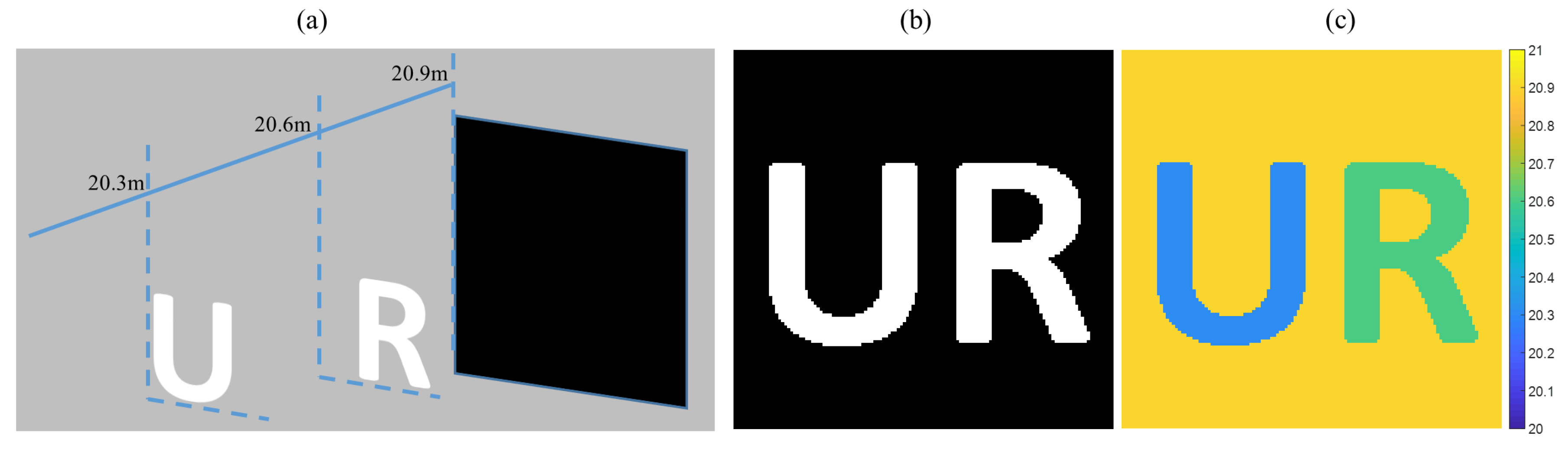
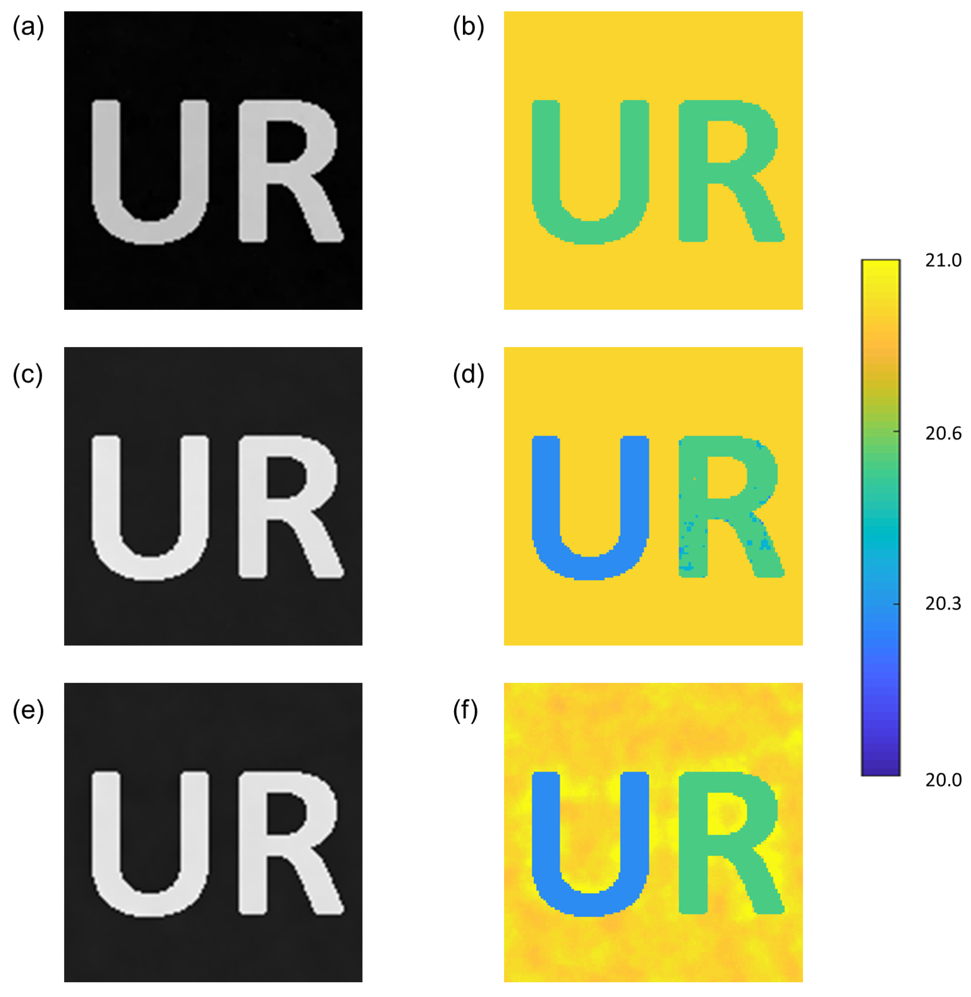
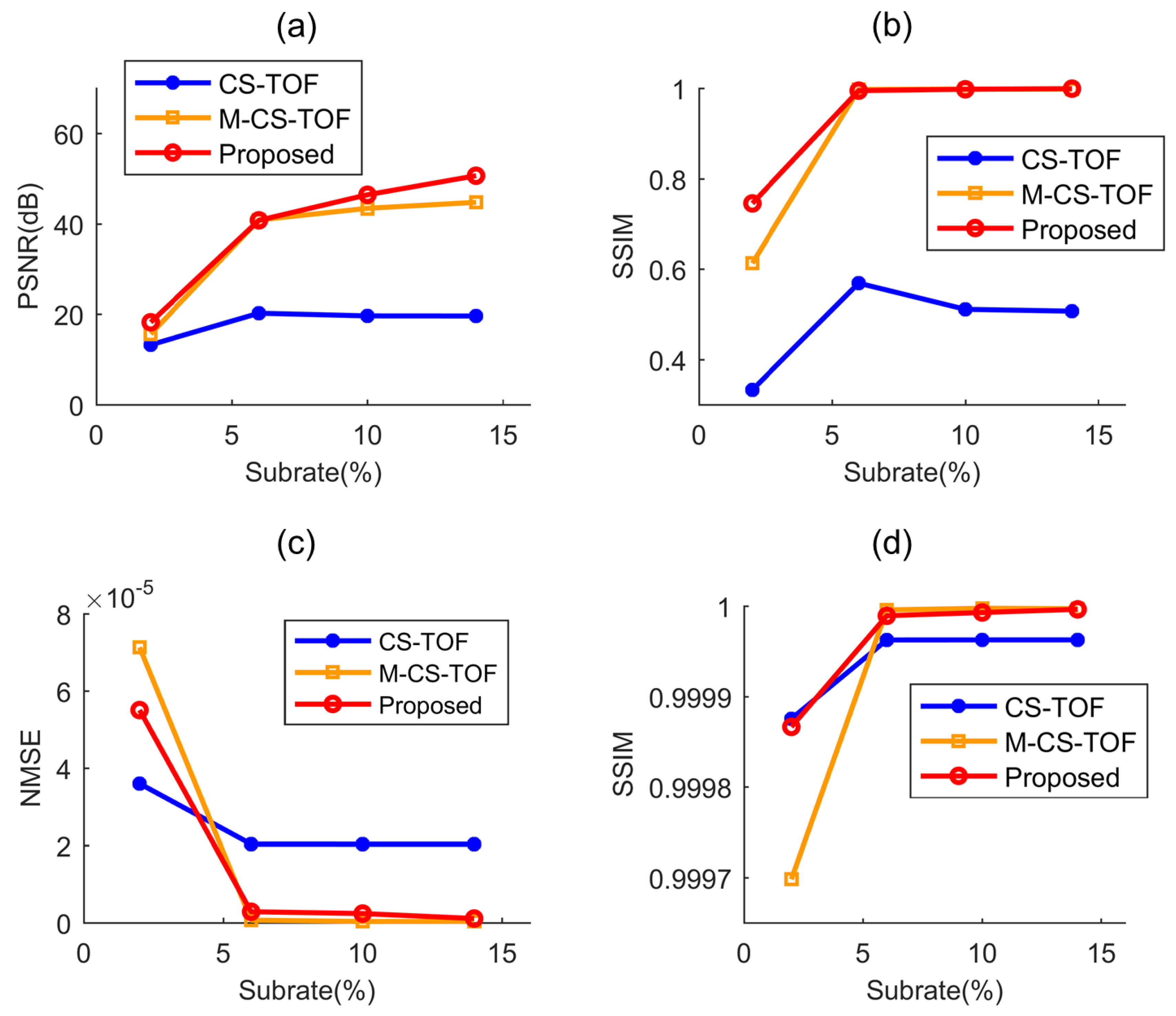
4.1. Reconstruction Performance of the Discrete Target

As shown in Figure 4a, a 3D scene is designed as the space discrete target which consists of two square cardboards cut-outs of the letters “U” and “R”. This is a typical target scene in CS-based 3D imaging [4,15,17,40]. The boards are distinguished and located parallelly at different positions in the scene. The distance between the RGI system and the cardboards ranges from 20.3 m to 20.9 m and therefore the gate opening range of 1 m is designated. The 3D scene is modeled by a combination of two matrices which are showed as the original intensity map, Figure 4b and the original depth map, Figure 4c. The original intensity map shows the reflectivity distribution of the target and the depth map shows the distance between each pixel of the target and the imaging system. In Figure 4c, colors correspond to the distance and the bar on the right side is added as an annotation.

The visual comparison of the imaging results of the “U & R” target scene by various methods is given in Figure 5. The measurements are in the presence of white Gaussian noise with SNR = 30 dB and all of the subrates equal to 10%. Colors correspond to the distance from 20.0 m to 21.0 m and the bar on the right side is added as an annotation. Figure 5a,c,e is the reconstructed intensity maps of the target applying CS-TOF, M-CS-TOF and the proposed method, respectively. These figures show that due to the full use of the CS framework, high-quality intensity maps are obtained which not only describe the shape feature of the scene but also have the edge detail of the target. Figure 5b is the reconstructed depth map from the measurements applying CS-TOF. The letters, “U” and “R”, stand out from the background in the figure but most pixels in them have similar depth values. It means the CS-TOF approach fails to successfully recover the scene in this system. Figure 5d is the reconstructed depth map of multiple planar objects applying M-CS-TOF. Two letters at separate positions are successfully recovered, the depth of each pixel in the target is determined accurately except for some acceptable noise. For a specific subrate, two intensity images containing range information are reconstructed in CS framework by two sets of measurements modulated with $g_{in}\left(t\right)$ and $g_{de}\left(t\right)$, respectively. A depth map of the target scene can be obtained from them by the proposed method. Figure 5f is the reconstructed map of the objects at separate positions with unknown depth by applying the proposed method. The object planes and edges are recovered accurately to demonstrate the depth and transverse resolution which indicates the feasibility of the proposed method.

Given subjective observation of the reconstructed maps, Peak Signal to Noise Ratio (PSNR) criterion, Normalized Mean Squared Error (NMSE) metric and a measure of Structural SIMilarity (SSIM) are adopted to assess the reconstruction quality as shown in Figure 6. A standard definition of the PSNR for the reconstructed intensity map $\widehat{x}$ and the original intensity map x is of the form:

$$PSNR\left(\widehat{x},x\right)\left(dB\right)=10{log}_{10}\frac{N·max{\left(x\right)}^2}{{\sum }_{i=1}^N{\left(\widehat{x}\left(i\right)-x\left(i\right)\right)}^2},$$

(28)

where N is the total number of pixels in x, $\widehat{x}\left(i\right)$ and $x\left(i\right)$ are the intensity of the ith pixel corresponding to the reconstructed intensity maps and the original intensity maps, respectively [41]. NMSE is adopted to compare the reconstructed depth maps with the original depth map:

$$NMSE\left(\widehat{d},d\right)=\frac{{\sum }_{i=1}^N{\left(d\left(i\right)-\widehat{d}\left(i\right)\right)}^2}{{\sum }_{i=1}^N{\left(d\left(i\right)\right)}^2},$$

(29)

where $d\left(i\right)$ and $\widehat{d}\left(i\right)$ are the depth of the ith pixel corresponding to the original depth maps and the estimated depth maps, respectively [42].

Besides the criterion above which have clear physical meanings in context of optimization, another kind of criterion is adopted that is well matched to perceived visual quality for extracting structural information. SSIM is widely used by comparing local patterns of pixels after normalized for illuminance and contrast. The index is in a specific form as follows:

$$SSIM(x,\widehat{x})=\frac{\left(2{\mu }_x{\mu }_{\widehat{x}}+C_1\right)\left(2{\sigma }_{x\widehat{x}}+C_2\right)}{({\mu }_x^2+{\mu }_{\widehat{x}}^2+C_1)({\sigma }_x^2+{\sigma }_{\widehat{x}}^2+C_2)},$$

(30)

where ${\mu }_{*}$ is the mean of the image, ${\sigma }_{*}$ is the standard deviation, $C_1$ and $C_2$ are constant to avoid instability under certain circumstances [43]. The index ranges from 0 to 1 and it equals to 1 when two images are exactly the same.

Figure 6 provide the objective assessment of reconstruction qualities of the “U & R” target scene in the presence of white Gaussian noise with SNR = 30 dB. Figure 6a presents the plots of the PSNR values for reconstructed intensity maps on various subrates (from 2% to 14%) using different approaches. It shows that PSNRs of the proposed method are always higher than those of the TOF-based methods as the subrates increase. The plots corresponding to M-CS-TOF and the proposed method stay stubbornly high and the PSNRs are more than 40 dB when the subrates reach 6% so that high-quality intensity maps are achieved. However, the PSNRs of the CS-TOF reconstructing intensity maps are much lower which results from the error of measurements caused by the echo pulses with different delays overlapping each other. Figure 6b presents the plots of the SSIM values for reconstructed intensity maps on various subrates (from 2% to 14%) using different approaches. The plots corresponding to M-CS-TOF and the proposed method stay stubbornly high and the SSIMs are close to 1 when the subrates reach 6% so that the structures of the target and the reconstructed image are extraordinary similar. On the contrary, the SSIMs of the CS-TOF reconstructing intensity maps are much lower. The SSIMs show similar pattern to the PSNR results, further verify the effectiveness and advantage of the proposed method. Figure 6c presents the plots of the NMSE values for reconstructed depth maps on various subrates (from 2% to 14%) using different approaches. It shows that NMSEs of M-CS-TOF and the proposed method are extremely low especially when the subrates reach 6%. These two methods are feasible and high-quality depth maps are achieved. There are significant errors in the depth maps reconstructed by CS-TOF because it fails to conduct multiple peak detection in overlapped echo pulses. Figure 6d presents the plots of the SSIM values for reconstructed depth maps on various subrates (from 2% to 14%) using different approaches. All of the SSIMs are close to 1 because the structures of the depth distribution are simple and the targets are located at only two unique distances. Still, the performance of the proposed method is as good as M-CS-TOF as the subrate increases which surpass CS-TOF obviously. These quantitative comparisons clearly indicate that the proposed method consistently surpasses CS-TOF and achieves the same effect with M-CS-TOF.

From both subjective observation and objective assessment in the above-mentioned, we can assert that the proposed 3D recover method is effective for discrete 3D targets imaging.

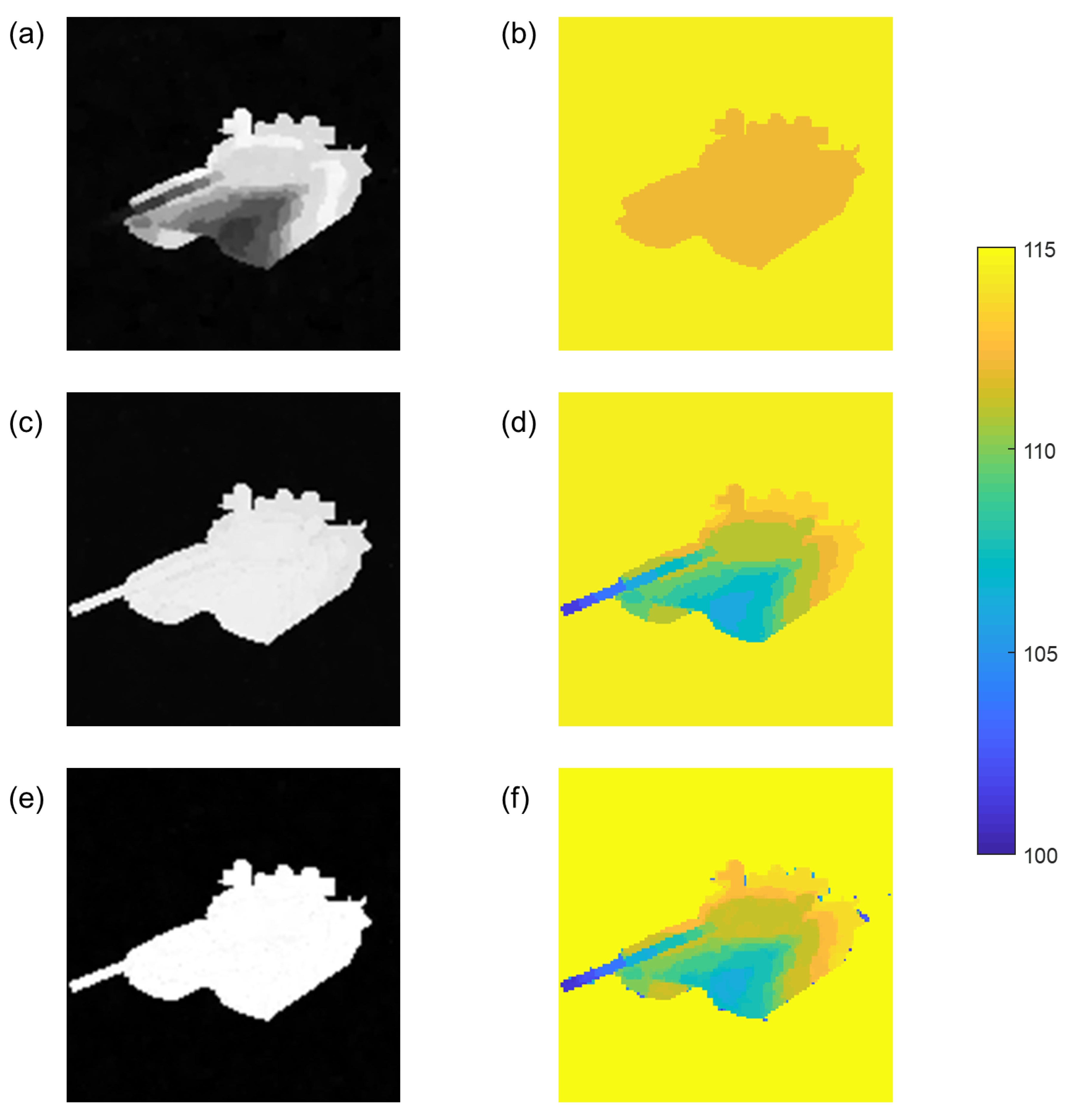
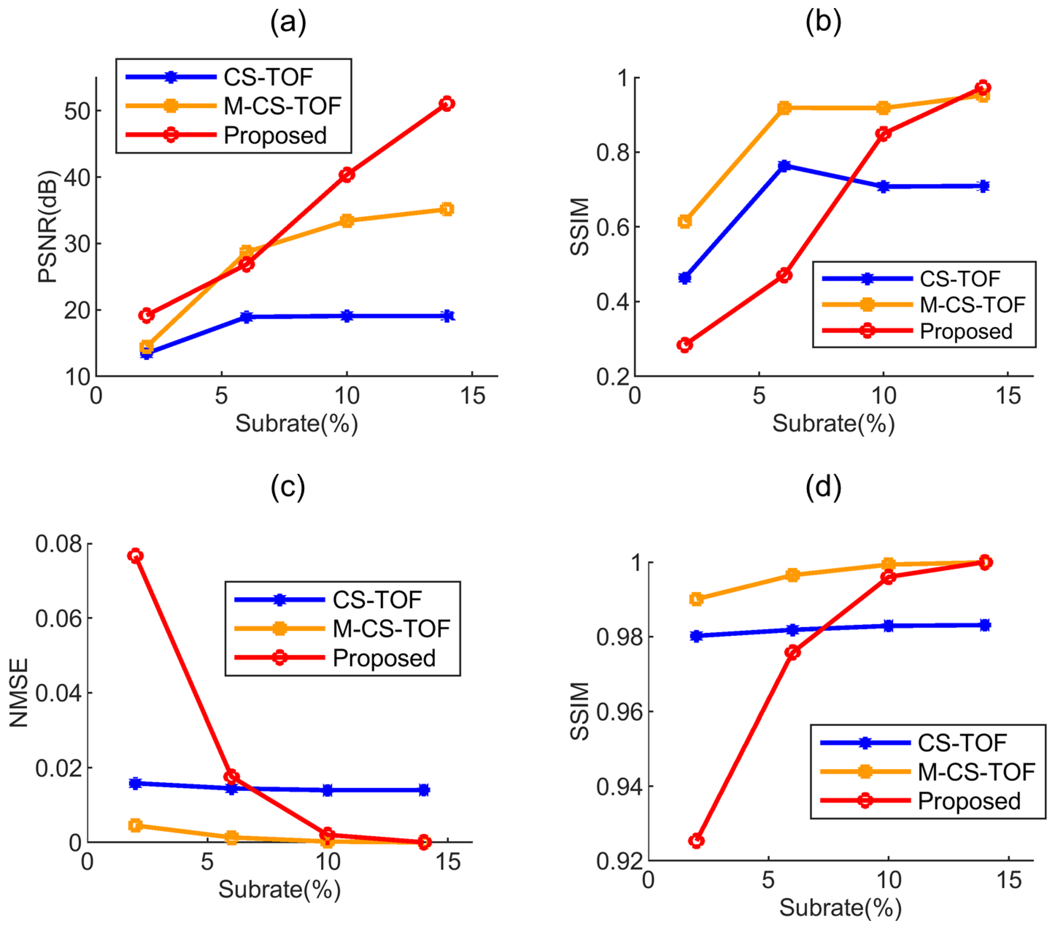
4.2. Reconstruction Performance of the Continuous Target

As is shown in Figure 7a, a 3D scene is designed as the space continuous target which is a 3D model of a tank T80. Observing from the left anterior of the tank, its entire length is more than 10 m long. The distance between the tank and RGI system is about 100 m and therefore the gate opening range of 15 m is designed. The 3D scene is modeled by a combination of two matrices which are showed as the original intensity map, Figure 7b and the original depth map, Figure 7c. In Figure 7c, colors correspond to the distance and the bar on the right side is added as an annotation.

The visual comparison of the imaging results of the T80 target scene by various methods is given in Figure 8. The measurements are in the presence of white Gaussian noise with SNR = 30 dB and all of the subrates are equal to 10%. Colors correspond to the distance from 100.0 m to 115.0 m and the bar on the right side is added as an annotation.

Figure 8a shows the reconstructed intensity maps of the target applying CS-TOF. There is a big error in terms of the pixel values and the structures of the target are incomplete between the result and the original intensity map. Figure 8c,e are the reconstructed intensity maps of the target applying M-CS-TOF and the proposed method, respectively. These figures show that due to the full use of the CS framework, high-quality intensity maps are obtained which not only describe the shape feature of the scene but also have the edge detail of the target. Figure 8b is the reconstructed depth map from the measurements applying CS-TOF. Unfortunately, the depth map is not only able to describe the integral outline of the target but also lacks the time-resolved ability. Figure 8d,f are the reconstructed depth maps of the continuous object applying M-CS-TOF and the proposed method. The object planes and edges are recovered well to demonstrate the depth and transverse resolution by determining the depth of each pixel accurately except for some acceptable noise. The errors in the edge of the object in Figure 8f result from some inaccurate pixels obtained in the optimization computation procedure, which will be eliminated as the subrate increases. The result indicates the feasibility of the proposed method.

Figure 9 provides the objective assessment of reconstruction qualities of the T80 target scene in the presence of white Gaussian noise with SNR = 30 dB. Figure 9a presents the plots of the PSNR values for reconstructed intensity maps on various subrates (from 2% to 14%) using different approaches.

It shows that PSNRs of the proposed method are always higher than those of the TOF-based methods as the subrates reach 10%. The plots corresponding to M-CS-TOF and the proposed method stay stubbornly high and the PSNRs are more than 30 dB so that high-quality intensity maps are achieved. However, the PSNRs of the CS-TOF reconstructing intensity maps are much lower which results from the error of the measurements used for reconstruction. The phenomenon that the echo pulses with different delays overlap each other always leads to significant reconstruction errors applying TOF-based methods. Figure 9b presents the plots of the SSIM values for reconstructed intensity maps on various subrates (from 2% to 14%) using different approaches. The plots corresponding to M-CS-TOF and the proposed method stay stubbornly high and the SSIMs are close to 1 when the subrates reach 10% so that the structures of the target and the reconstructed image are extraordinary similar. On the contrary, the SSIMs of the CS-TOF reconstructing intensity maps are much lower. With similar pattern to the PSNR results, the SSIMs further verify the effectiveness and advantage of the proposed method. Figure 9c presents the plots of the NMSE values for reconstructed depth maps on various subrates (from 2% to 14%) using different approaches. It shows that NMSEs of M-CS-TOF and the proposed method are extremely low especially when the subrates reach 10%. These two methods are feasible and high-quality depth maps are achieved. Figure 9d presents the plots of the SSIM values for reconstructed depth maps on various subrates (from 2% to 14%) using different approaches. The SSIMs are close to 1 when the subrates reach 10% except for CS-TOF. Both the pixel-wise and the structure-wise assessment demonstrates the reconstruction quality. Moreover, These quantitative comparisons clearly indicate that the proposed method consistently surpasses CS-TOF and achieves the comparative effect with M-CS-TOF.

From both subjective observation and objective assessment in the above-mentioned, we can assert that the proposed 3D recover method is effective for continuous 3D targets imaging.

Figure 10 provide the 3D reconstruction results of the “U & R” target with varying reflectance. The measurements are in the presence of white Gaussian noise with SNR = 30 dB and all of the subrates equal to 10%. Colors correspond to the distance from 20.0 m to 21.0 m and the bar on the right side is added as an annotation. The objects are with varying reflectance in the intensity map in Figure 10a,b is the depth map where two letters are at separated locations. The results demonstrate that the proposed method is effective for 3D imaging of targets with varying reflectance.

Table 2. Performance of several CS-based 3D imaging methods.

Imaging Methods	CS-TOF	M-CS-TOF	Proposed
FWHM	resolution related	free	free
Sampling rate	higher	higher	lower
Sets of measurements	some	dozens	2
Number of frames	some	dozens	2
Execution time	medium	long	short

is provided for comparison with the performance of several CS-based 3D imaging methods in terms of FWHM, sampling rate and the number of frames. To achieve a particular range resolution as is shown in the simulation above, the required parameters are given when each method is adopted respectively. The required width of the transmitting laser pulses is free and the required sampling frequency of the detector is lower because they are not directly relevant to the range resolution. It means that the proposed method can achieve range super-resolution to reconstruct the 3D scene when conventional methods are ineffective against the limitation of narrow-bandwidth pulsed lasers and high-frequency sampling. Moreover, a frame refers to an intensity image recovered from the measurements which are recorded from the total echo waveforms. Compared with conventional methods, the proposed method leads to smaller data sets and shorter measuring time that it can obtain specific range resolution with much fewer frames. Reconstructing only two frames to achieve 3D imaging reduces the computation expense resulting in a faster procedure.

5. Conclusions

In this paper, we presented a compressive sensing based electro-optic modulation method for nonscanning 3D laser imaging to overcome the limitations of traditional methods. Generally, the flying time values of laser pulses from multiple pixels do not possess linear properties which means they are not compressible. The proposed method transforms the flying time values into intensity values of the echo pulses through electro-optic modulation and peak values of the total echo pulses are recorded in CS framework. As a result, both the time and reflectivity information are compressible and can be reconstructed from much smaller sets of their linear projection. Two sets of CS measurements are obtained to recover the modulated images of the target when a monotone increasing and a monotone decreasing voltage functions are applied respectively. We formulate a minimization model integrated with a detail-preserving regularization and TV regularization for the inverse problem of image retrieval. Then we propose an ADMM imbedded algorithm to solve the unconstrainted regulated optimization problem efficiently. Finally, the 3D form of the target scene is completed as a combination of the intensity map and the depth map extracted from the two reconstructed images with gain modulation. The simulation results demonstrate that the proposed method is able to achieve high-quality 3D imaging for both the discrete target and the continuous target. More importantly, it has the advantage of range super-resolution with fewer required frames compared with CS-TOF method and M-CS-TOF method when echo pulses from targets with different ranges are indistinguishable. With fewer reconstructed frames in need, the proposed method requires less data for further processing, thus reducing the computation expense in reconstruction to achieve a faster performance. The research has important scientific value and is beneficial for the extensive application of 3D laser imaging such as low-cost LiDAR, high-speed image acquisition and remote sensing. A natural progression of this work is to build a realizable system for 3D imaging of various targets..

References

1. Molebny, V.; Mcmanamon, P.; Steinvall, O.; Kobayashi, T.; Chen, W. Laser radar: Historical prospective—From the East to the West. Opt. Eng. 2016, 56, 031220. [Google Scholar] [CrossRef]
2. Li, L.; Wu, L.; Wang, X.; Dang, E. Gated viewing laser imaging with compressive sensing. Appl. Opt. 2012, 51, 2706–2712. [Google Scholar] [CrossRef] [PubMed]
3. Gao, H.; Zhang, Y.; Guo, H. Multihypothesis-Based Compressive Sensing Algorithm for Nonscanning Three-Dimensional Laser Imaging. IEEE J. STARS 2018, 11, 311–321. [Google Scholar] [CrossRef]
4. Colaco, A.; Kirmani, A.; Howland, G.A.; Howell, J.C.; Goyal, V.K. Compressive Depth Map Acquisition Using a Single Photon-Counting Detector: Parametric Signal Processing Meets Sparsity. In Proceedings of the IEEE Conference on Computer Vision and Pattern Recognition, Providence, RI, USA, 16–21 June 2012; pp. 96–102. [Google Scholar] [CrossRef] [Green Version]
5. Gibson, G.M.; Sun, B.; Edgar, M.P.; Phillips, D.B.; Hempler, N.; Maker, G.T.; Malcolm, G.P.A.; Padgett, M.J. Real-time imaging of methane gas leaks using a single-pixel camera. Opt. Express 2017, 25, 2998–3005. [Google Scholar] [CrossRef] [PubMed]
6. Edgar, M.; Johnson, S.; Phillips, D.; Padgett, M. Real-time computational photon-counting LiDAR. Opt. Eng. 2018, 57, 031304. [Google Scholar] [CrossRef] [Green Version]
7. Sun, M.J.; Zhang, J.M. Single-Pixel Imaging and Its Application in Three-Dimensional Reconstruction: A Brief Review. Sensors 2019, 19, 732. [Google Scholar] [CrossRef] [Green Version]
8. Zhang, X.D.; Li, C.L.; Meng, Q.P.; Liu, S.J.; Zhang, Y.; Wang, J.Y. Infrared Image Super Resolution by Combining Compressive Sensing and Deep Learning. Sensors 2018, 18, 2587. [Google Scholar] [CrossRef] [Green Version]
9. Zhang, T.; Gao, K. MAP-MRF-based super-resolution reconstruction approach for coded aperture compressive temporal imaging. Appl. Sci. 2018, 8, 338. [Google Scholar] [CrossRef] [Green Version]
10. Donoho, D.L. Compressed sensing. IEEE T. Inform. Theory 2006, 52, 1289–1306. [Google Scholar] [CrossRef]
11. Candès, E.J. Compressive sampling. In Proceedings of the International Congress of Mathematicians, Madrid, Spain, 22–30 August 2006; Volume 3, pp. 1433–1452. [Google Scholar]
12. Rani, M.; Dhok, S.B.; Deshmukh, R.B. A Systematic Review of Compressive Sensing: Concepts, Implementations and Applications. IEEE Access 2018, 6, 4875–4894. [Google Scholar] [CrossRef]
13. Gan, H.P.; Xiao, S.; Zhang, T.; Zhang, Z.M.; Li, J.; Gao, Y. Chaotic Pattern Array for Single-Pixel Imaging. Electronics 2019, 8, 536. [Google Scholar] [CrossRef] [Green Version]
14. Duarte, M.F.; Davenport, M.A.; Takhar, D.; Laska, J.N.; Sun, T.; Kelly, K.F.; Baraniuk, R.G. Single-pixel imaging via compressive sampling. IEEE Signal Proc. Mag. 2008, 25, 83–91. [Google Scholar] [CrossRef] [Green Version]
15. Howland, G.A.; Dixon, P.B.; Howell, J.C. Photon-counting compressive sensing laser radar for 3D imaging. Appl. Opt. 2011, 50, 5917–5920. [Google Scholar] [CrossRef] [PubMed] [Green Version]
16. Sun, M.J.; Edgar, M.P.; Gibson, G.M.; Sun, B.; Radwell, N.; Lamb, R.; Padgett, M.J. Single-pixel three-dimensional imaging with time-based depth resolution. Nat. Commun. 2016, 7. [Google Scholar] [CrossRef] [PubMed]
17. Howland, G.A.; Lum, D.J.; Ware, M.R.; Howell, J.C. Photon counting compressive depth mapping. Opt. Express 2013, 21, 23822–23837. [Google Scholar] [CrossRef] [PubMed] [Green Version]
18. Busck, J.; Heiselberg, H. Gated viewing and high-accuracy three-dimensional laser radar. Appl. Opt. 2004, 43, 4705–4710. [Google Scholar] [CrossRef] [PubMed]
19. Laurenzis, M.; Christnacher, F.; Monnin, D. Long-range three-dimensional active imaging with superresolution depth mapping. Opt. Lett. 2007, 32, 3146–3148. [Google Scholar] [CrossRef]
20. Jin, C.; Sun, X.; Zhao, Y.; Zhang, Y.; Liu, L. Gain-modulated three-dimensional active imaging with depth-independent depth accuracy. Opt. Lett. 2009, 34, 3550–3552. [Google Scholar] [CrossRef]
21. Tsagkatakis, G.; Woiselle, A.; Tzagkarakis, G.; Bousquet, M.; Starck, J.L.; Tsakalides, P. Multireturn compressed gated range imaging. Opt. Eng. 2015, 54, 031106. [Google Scholar] [CrossRef] [Green Version]
22. Wang, X.; Li, Y.; Zhou, Y. Multi-pulse time delay integration method for flexible 3D super-resolution range-gated imaging. Opt. Express 2015, 23, 7820–7831. [Google Scholar] [CrossRef]
23. Laurenzis, M.; Becher, E. Three-dimensional laser-gated viewing with error-free coding. Opt. Eng. 2018, 57, 7. [Google Scholar] [CrossRef]
24. Chen, Z.; Liu, B.; Liu, E.; Peng, Z. Electro-optic modulation methods in range-gated active imaging. Appl. Opt. 2016, 55, A184–A190. [Google Scholar] [CrossRef]
25. An, Y.; Zhang, Y.; Guo, H.; Wang, J. Compressive Sensing-Based Three-Dimensional Laser Imaging With Dual Illumination. IEEE Access 2019, 7, 25708–25717. [Google Scholar] [CrossRef]
26. Fade, J.; Perrotin, E.; Bobin, J. Polarizer-free two-pixel polarimetric camera by compressive sensing. Appl. Opt. 2018, 57, B102–B113. [Google Scholar] [CrossRef] [PubMed] [Green Version]
27. Zhang, Y.L.; Suo, J.L.; Wang, Y.W.; Dai, Q.H. Doubling the pixel count limitation of single-pixel imaging via sinusoidal amplitude modulation. Opt. Express 2018, 26, 6929–6942. [Google Scholar] [CrossRef] [PubMed]
28. Chen, Z.; Liu, B.; Liu, E.; Peng, Z. Adaptive Polarization-Modulated Method for High-Resolution 3D Imaging. IEEE Photonic Technol. Lett. 2016, 28, 295–298. [Google Scholar] [CrossRef]
29. Gao, H.; Zhang, Y.-M.; Guo, H.-C. A compressive sensing algorithm using truncated SVD for three-dimensional laser imaging of space-continuous targets. J. Mod. Optic. 2016, 63, 2166–2172. [Google Scholar] [CrossRef]
30. Duarte, M.F.; Baraniuk, R.G. Kronecker Compressive Sensing. IEEE Trans. Image Process. 2012, 21, 494–504. [Google Scholar] [CrossRef]
31. Buyssens, P.; Daisy, M.; Tschumperle, D.; Lezoray, O. Exemplar-Based Inpainting: Technical Review and New Heuristics for Better Geometric Reconstructions. IEEE Trans. Image Process. 2015, 24, 1809–1824. [Google Scholar] [CrossRef]
32. Duarte, M.F.; Sarvotham, S.; Baron, D.; Wakin, M.B.; Baraniuk, R.G. Distributed compressed sensing of jointly sparse signals. In Proceedings of the Conference Record of the Thirty-Ninth Asilomar Conference onSignals, Systems and Computers, Pacific Grove, CA, USA, 30 October–2 November 2005; pp. 1537–1541. [Google Scholar]
33. Candes, E.J.; Wakin, M.B. An introduction to compressive sampling. IEEE Signal Proc. Mag. 2008, 25, 21–30. [Google Scholar] [CrossRef]
34. Bhattacharjee, T.; Maity, S.P. Progressive and hierarchical share-in-share scheme over cloud. J. Inf. Secur. Appl. 2019, 46, 108–120. [Google Scholar] [CrossRef]
35. Bian, L.H.; Suo, J.L.; Dai, Q.H.; Chen, F. Experimental comparison of single-pixel imaging algorithms. J. Opt. Soc. Am. A 2018, 35, 78–87. [Google Scholar] [CrossRef] [PubMed]
36. Guo, W.; Qin, J.; Yin, W. A New Detail-Preserving Regularization Scheme. SIAM J. Imaging Sci. 2014, 7, 1309–1334. [Google Scholar] [CrossRef]
37. Boyd, S.; Parikh, N.; Chu, E.; Peleato, B.; Eckstein, J. Distributed optimization and statistical learning via the alternating direction method of multipliers. Found. Trends® Mach. Learn. 2011, 3, 1–122. [Google Scholar] [CrossRef]
38. Li, C. An Efficient Algorithm for Total Variation Regularization with Applications to the Single Pixel Camera and Compressive Sensing. Master’s Thesis, Department of Computational and Applied Mathematics, Houston, TX, USA, 2009. [Google Scholar]
39. Li, F.; Chen, H.; Pediredla, A.; Yeh, C.; He, K.; Veeraraghavan, A.; Cossairt, O. CS-ToF: High-resolution compressive time-of-flight imaging. Opt. Express 2017, 25, 31096–31110. [Google Scholar] [CrossRef] [Green Version]
40. Kirmani, A.; Colaço, A.; Wong, F.N.; Goyal, V.K. Exploiting sparsity in time-of-flight range acquisition using a single time-resolved sensor. Opt. Express 2011, 19, 21485–21507. [Google Scholar] [CrossRef]
41. Czajkowski, K.M.; Pastuszczak, A.; Kotynski, R. Single-pixel imaging with Morlet wavelet correlated random patterns. Sci. Rep. 2018, 8, 8. [Google Scholar] [CrossRef] [Green Version]
42. Marques, E.C.; Maciel, N.; Naviner, L.; Cai, H.; Yang, J. A Review of Sparse Recovery Algorithms. IEEE Access 2019, 7, 1300–1322. [Google Scholar] [CrossRef]
43. Wang, Z.; Bovik, A.C.; Sheikh, H.R.; Simoncelli, E.P. Image quality assessment: From error visibility to structural similarity. IEEE T. Image Process. 2004, 13, 600–612. [Google Scholar] [CrossRef] [Green Version]
Figure 1. Schematic diagram of the proposed compressive sensing RGI system.
Symmetry 12 00748 g001
Figure 2. The time sequence of gain modulation for the RGI system: (a) time sequence of receiver gate, applied voltage of the EOM, gain function, laser pulse, and received pulse of APD; (b) received pulse and its subpulses with gain function g i n ( t ) ; (c) received pulse and its subpulses with gain function g d e ( t ) .
Symmetry 12 00748 g002
Figure 3. Schematic diagram of electro-optic modulation.
Symmetry 12 00748 g003
Figure 4. 3D scene ranged from 20.3 m to 20.9 m: (a) the conceptual graph of the “U & R” target; (b) the original intensity map; (c) the original depth map.
Symmetry 12 00748 g004
Figure 5. The 3D reconstruction results of the “U & R” target scene by various methods: (a) the reconstructed intensity map by CS-TOF; (b) the reconstructed depth map by CS-TOF; (c) the reconstructed intensity map by M-CS-TOF; (d) the reconstructed depth map by M-CS-TOF; (e) the reconstructed intensity map by the proposed method; (f) the reconstructed depth map by the proposed method.
Symmetry 12 00748 g005
Figure 6. The objective assessment of reconstruction qualities of the “U & R” target scene using different approaches: (a) the plots of PSNR for reconstructed intensity maps as a function of subrates; (b) the plots of SSIM for reconstructed intensity maps as a function of subrates; (c) the plots of NMSE for reconstructed depth maps as a function of subrates; (d) the plots of SSIM for reconstructed depth maps as a function of subrates.
Symmetry 12 00748 g006
Figure 7. 3D scene ranged from 100 m to 115 m: (a) a 3D model of a tank T80 in the target scene; (b) the original intensity map; (c) the original depth map.
Symmetry 12 00748 g007
Figure 8. The 3D reconstruction results of the T80 target scene by various methods: (a) the reconstructed intensity map by CS-TOF; (b) the reconstructed depth map by CS-TOF; (c) the reconstructed intensity map by M-CS-TOF; (d) the reconstructed depth map by M-CS-TOF; (e) the reconstructed intensity map by the proposed method; (f) the reconstructed depth map by the proposed method.
Symmetry 12 00748 g008
Figure 9. The objective assessment of reconstruction qualities of the T80 target scene using different approaches: (a) the plots of PSNR for reconstructed intensity maps as a function of subrates; (b) the plots of SSIM for reconstructed intensity maps as a function of subrates; (c) the plots of NMSE for reconstructed depth maps as a function of subrates; (d) the plots of SSIM for reconstructed depth maps as a function of subrates.
Symmetry 12 00748 g009
Figure 10. The 3D reconstruction results of the “U & R” target with varying reflectance: (a) the reconstructed intensity map; (b) the reconstructed depth map.
Symmetry 12 00748 g010