M-Polynomial and Degree Based Topological Indices of Some Nanostructures

Abstract

The association of M-polynomial to chemical compounds and chemical networks is a relatively new idea, and it gives good results about the topological indices. These results are then used to correlate the chemical compounds and chemical networks with their chemical properties and bioactivities. In this paper, an effort is made to compute the general form of the M-polynomials for two classes of dendrimer nanostars and four types of nanotubes. These nanotubes have very nice symmetries in their structural representations, which have been used to determine the corresponding M-polynomials. Furthermore, by using the general form of M-polynomial of these nanostructures, some degree-based topological indices have been computed. In the end, the graphical representation of the M-polynomials is shown, and a detailed comparison between the obtained topological indices for aforementioned chemical structures is discussed.

1. Introduction and Preliminaries

A molecular graph (in chemical graph theory) is a simple graph (a graph that does not contain edges whose two ends are the same vertex, nor containing two edges with the same two ends) where the atoms of the molecule are represented as vertices and the bonds between them are the edges. A graph $G(V,E)$ consists of a vertex set $V(G)$ and an edge set $E(G)$. The number of edges incident to v of some vertex of a graph G is said to be its degree and is denoted by $d_v$; $\delta$ is the minimum degree of a graph, and $\Delta$ is its maximum. We can represent an edge with vertices, $e=uv\in E(G)$, if it connects vertex u to vertex v.

Topological indices are a numerical quantity computed from the molecular graph of a chemical compound and typically remain the same under graph isomorphism. A topological index determined by means of using the degrees of the molecular graph is a family of indices that can be used to point out and model certain properties of chemical compounds; these indices are also known as degree-based topological indices [1,2,3,4]. In the same context, the M-polynomial plays a similar part; we can obtain closed-form formulas for degree-based topological indices from it [5,6,7,8,9,10].

There are some recent papers devoted to the computation of the M-polynomial of a given chemical graph. In particular, in [11], the authors considered two infinite classes $NS1\left[n\right]$ and $NS2\left[n\right]$ of nanostar dendrimers and computed the Zagreb indices and Zagreb polynomials for these special nanostar dendrimers. In [12], the author determined certain Zagreb polynomials of a special type of dendrimer nanostar $D_3\left[n\right]$, and the Zagreb indices and Zagreb polynomials of the same dendrimer nanostars were computed in [13]. The computation of some fifth multiplicative Zagreb indices of PAMAMdendrimers was reported in [14]. The first and second reverse Zagreb indices, reverse hyper-Zagreb indices, and their polynomials of porphyrin, propyl ether imine, zinc porphyrin, and poly(ethylene amido amine) dendrimers were determined in [15]. The computation of the M-polynomial and topological indices of the benzene ring embedded in a P-type surface network was given in [16]. The M-polynomial and degree-based topological indices of polyhex nanotubes were given in [9]. The main object of this paper is to derive the general form of the M-polynomial for two dendrimer nanostars $N{D}_1\left[n\right]$, $N{D}_2\left[n\right]$ (Figure 1A,B) and four types of nanotubes. Furthermore, we compute the first and second Zagreb index, the modified Zagreb index, the Randic index, and the symmetric division index for this family of molecules. We also give the graphical representation of the M-polynomial. A comparison between the obtained topological indices of these chemical graphs is outlined at the end.

2. Materials and Methods

Dendrimers are repetitively branching artificial star-shaped molecules synthesized from branched units called monomers using a nanoscale fabrication process; they have a well-defined structure with three major components: the core, branches, and end groups, where new branches are made from the core and are added recursively in steps. There are various applications of nanostar dendrimers for the formation of micro- and macro-capsules, chemical sensors, colored glasses, and modified electrodes. Due to these applications, these compounds have attracted much attention in both chemistry and mathematics alike.

Nanotubes are a nanoscale material that takes up a tube-like structure and can be made from various materials, organic or inorganic, such as carbon, boron, and silicon. CNT (Carbon Nanotubes) have a high thermal and electrical conductivity, while also being highly flexible and being good electron field emitters. They have various applications in energy storage, air and water filtration, fabrics, and thermal compounds and have attracted much attention from the scientific community.

Boron nanotubes are attracting much attention as well because of their remarkable properties such as structural stability, work function, transport properties, and electronic structure and are coming to challenge CNTs. In this article, we study the structures of two configurations of CNT, “zig-zag” $G_1[n,m]$ and “armchair” $G_2[n,m]$ (Figure 2A,B), and two kinds of Boron nanotubes, triangular boron $G_3[n,m]$ and $\alpha$-boron $G_4[n,m]$ (Figure 3A,B).

As introduced by Grutman and Trinajstic, the first Zagreb index $M_1(G)$ and the second Zagreb index $M_2(G)$ are defined as follows [17]:

$$M_1(G)=\sum _{v\in V(G)}{d}_v^2,M_2(G)=\sum _{vw\in E(G)}{d}_v{d}_w.$$

It is well known that the first Zagreb index can be written as:

$$M_1(G)=\sum _{vw\in E(G)}(d_v+d_w).$$

The modified Zagreb index ${}^m{M}_2(G)$ is defined to be:

$${}^m{M}_2(G)=\sum _{vw\in E(G)}\frac{1}{d_v{d}_w}$$

$R_{\alpha }(G)$, the general Randic index, is defined to be:

$$R_{\alpha }(G)=\sum _{vw\in E(G)}{(d_v{d}_w)}^{\alpha }$$

where $\alpha \in \mathbb{R}$.

The symmetric division index, $SDD(G)$, is defined to be:

$$SDD(G)=\sum _{vw\in E(G)}(\frac{d_v}{d_w}+\frac{d_w}{d_v})=\sum _{vw\in E(G)}\frac{d_v^2+d_w^2}{d_v{d}_w}$$

Let G be a simple molecular connected graph, and let $d_w$ denote the degree of some vertex $v\in V(G)$. The vertex set $V(G)$ can be partitioned as follows:

$$V(G)={\cup }_{\delta ⩽k⩽\Delta }{V}_k$$

where $V_k=\{v\in V(G)|d_v=k\}$. The edge set $E(G)$ can be partitioned into the following sets:

$$E_{(i,j)}=\{e=vw\in E(G)|d_v=i\&d_w=j\}$$

Then, the M-polynomial of a graph G denoted as $M(G,x,y)$ is defined to be:

$$M(G,x,y)=\sum _{\delta ⩽i⩽j⩽\Delta }{m}_{i,j}{x}^i{y}^j$$

where $m_{i,j}=\left|E_{(i,j)}\right|$.

From the above polynomial, one can obtain numerous degree-based topological indices by differentiating and/or integrating with respect to x and y [6]. The

Table 1. Derivation of degree-based topological indices form M-polynomial.

Topological Index	$\mathit{g}(\mathit{x},\mathit{y})$	Derivation from $\mathit{M}(\mathit{G},\mathit{x},\mathit{y})$
$M_1(G)$	$x+y$	${\left[(D_x+D_y)(M(G,x,y))\right]}_{(x,y)=(1,1)}$
$M_2(G)$	$xy$	${\left[(D_x{D}_y)(M(G,x,y))\right]}_{(x,y)=(1,1)}$
${}^m{M}_2(G)$	$\frac{1}{xy}$	${\left[(S_x{S}_y)(M(G,x,y))\right]}_{(x,y)=(1,1)}$
$R_{\alpha }(G)$	${(xy)}^{\alpha }$	${\left[(D_x^{\alpha }{D}_y^{\alpha })(M(G,x,y))\right]}_{(x,y)=(1,1)}$
$R_{\alpha }(G)$	$\frac{1}{{(xy)}^{\alpha }}$	${\left[(S_x^{\alpha }{S}_y^{\alpha })(M(G,x,y))\right]}_{(x,y)=(1,1)}$
$SDD(G)$	$\frac{x^2+y^2}{xy}$	${\left[(S_x{D}_y+S_y{D}_x)(M(G,x,y))\right]}_{(x,y)=(1,1)}$

below lists some of the degree-based topological indices and how to derived them from the M-polynomial.

where $D_x,D_y,S_x,S_y$ is defined to be:

$$\begin{array}{cccc}\hfill D_x(g(x,y))& =x\times \frac{\partial g(x,y)}{\partial x}\hfill & \hfill D_y(g(x,y))& =y\times \frac{\partial g(x,y)}{\partial y}\hfill \\ \hfill S_x(g(x,y))& =\int \frac{g(x,y)}{x}dx\hfill & \hfill S_y(g(x,y))& =\int \frac{g(x,y)}{y}dy\hfill \end{array}$$

3. Results

We found the M-polynomials of two special families of dendrimer nanostars denoted by $N{D}_1\left[n\right]\mathrm{and}N{D}_2\left[n\right]$ and four types of nanotubes denoted by $G_k[n,m]$ ($k=1,2,3,4$). After that, we represented some of the M-polynomials as three-dimensional surfaces using Mathematica, then with the assistance of the above table, we found the topological indices of the aforementioned structures.

3.1. M-Polynomials of the Dendrimer Nanostars

The main objective of this subsection is to obtain the general closed form of the M-polynomial associated with the two special nanostar dendrimers ($N{D}_1\left[n\right]\&N{D}_2\left[n\right]$).

Theorem 1.

Let $N{D}_1\left[n\right]$ be the molecular graph whose structure can be seen in Figure 1A. Then, its M-polynomial is:

$$M(N{D}_1\left[n\right],x,y)=(12\times 2^{n-1})x^2{y}^2+(24\times 2^{n-1}-12)x^2{y}^3+(6\times 2^{n-1}-3)x^3{y}^3$$

Proof. 

Studying the construction of $N{D}_1\left[n\right]$ (see Figure 1A), we can see that there are two partitions of the vertex set of $N{D}_1\left[n\right]$ as: $V_2=\{v\in V(N{D}_1\left[n\right])|d_v=2\}$ and $V_3=\{v\in V(N{D}_1\left[n\right])|d_v=3\}$. We also see that $E(N{D}_1\left[n\right])$ can be partitioned as follows:

$$\begin{array}{cc}\hfill E_{(2,2)}& =\{e=xy\in E(N{D}_1\left[n\right])|d_x=2\&d_y=2\}\hfill \\ \hfill E_{(2,3)}& =\{e=xy\in E(N{D}_1\left[n\right])|d_x=2\&d_y=3\}\hfill \\ \hfill E_{(3,3)}& =\{e=xy\in E(N{D}_1\left[n\right])|d_x=3\&d_y=3\}\hfill \end{array}$$

$\Rightarrow |E_{(2,2)}|=12\times 2^{n-1}$, $|E_{(2,3)}|=24\times 2^{n-1}-12$, and $|E_{(3,3)}|=6\times 2^{n-1}-3$. Thus, following from the definition, the M-polynomial of $N{D}_1\left[n\right]$ is:

$$\begin{array}{cc}\hfill M(N{D}_1\left[n\right],x,y)& =\sum _{i\le j}{m}_{i,j}(N{D}_1\left[n\right])x^i{y}^j\hfill \\ \hfill & =m_{2,2}(N{D}_1\left[n\right])x^2{y}^2+m_{2,3}(N{D}_1\left[n\right])x^2{y}^3\&+m_{3,3}(N{D}_1\left[n\right])x^3{y}^3\hfill \\ \hfill & =(12\times 2^{n-1})x^2{y}^2+(24\times 2^{n-1}-12)x^2{y}^3+(6\times 2^{n-1}-3)x^3{y}^3\hfill \end{array}$$

 □

Theorem 2.

Let $N{D}_2\left[n\right]$ be the molecular graph whose structure can be seen in Figure 1B. Then, its M-polynomial is:

$$M(N{D}_2\left[n\right],x,y)=(56\times 2^n-48)x^2{y}^2+(48\times 2^n-44)x^2{y}^3+(36\times 2^n-35)x^3{y}^3$$

Proof. 

Studying the construction of $N{D}_2\left[n\right]$ (see Figure 2B), we can see that there are two partitions of the vertex set of $N{D}_2\left[n\right]$ as: $V_2=\{v\in V(N{D}_2\left[n\right])|d_v=2\}$ and $V_3=\{v\in V(N{D}_2\left[n\right])|d_v=3\}$. We also see that $E(N{D}_2\left[n\right])$ can be partitioned as follows:

$$\begin{array}{cc}\hfill E_{(2,2)}& =\{e=xy\in E(N{D}_2\left[n\right])|d_x=2\&d_y=2\}\hfill \\ \hfill E_{(2,3)}& =\{e=xy\in E(N{D}_2\left[n\right])|d_x=2\&d_y=3\}\hfill \\ \hfill E_{(3,3)}& =\{e=xy\in E(N{D}_2\left[n\right])|d_x=3\&d_y=3\}\hfill \end{array}$$

$\Rightarrow |E_{(2,2)}|=56\times 2^n-48$, $|E_{(2,3)}|=48\times 2^n-44$, and $|E_{(3,3)}|=36\times 2^n-35$. Thus, following straight from the definition, the M-polynomial of $N{D}_2\left[n\right]$ is:

$$\begin{array}{cc}\hfill M(N{D}_2\left[n\right],x,y)& =\sum _{i\le j}{m}_{i,j}(N{D}_2\left[n\right])x^i{y}^j\hfill \\ \hfill & =m_{2,2}(N{D}_2\left[n\right])x^2{y}^2+m_{2,3}(N{D}_2\left[n\right])x^2{y}^3+m_{3,3}(N{D}_2\left[n\right])x^3{y}^3\hfill \\ \hfill & =(56\times 2^n-48)x^2{y}^2+(48\times 2^n-44)x^2{y}^3+(36\times 2^n-35)x^3{y}^3\hfill \end{array}$$

 □

3.2. M-Polynomials of the Nanotubes

In this subsection, we will provide the general formula for the M-polynomial of the four nanotubes ($G_k[n,m]$, where $k=1,2,3,4$), as shown in Figure 2A,B and Figure 3A,B. We also provide the graphical representation of these M-polynomials.

Theorem 3.

Let $G_1[n,m]$ be a molecular graph whose structure can be seen in Figure 2A. Then:

$$M(G_1[n,m],x,y)=2m{x}^2{y}^3+(\frac{m}{2}(3n-5))x^3{y}^3$$

Proof. 

Studying the construction of $G_1[n,m]$, we can see that there are two partitions of the vertex set of $G_1[n,m]$ as: $V_2=\{v\in V(G_1[n,m])|d_v=2\}$ and $V_3=\{v\in V(G_1[n,m])|d_v=3\}$. We also see that $E(G_1[n,m])$ can be partitioned as follows:

$$\begin{array}{cc}\hfill E_{(2,3)}& =\{e=xy\in E(G_1[n,m]])|d_x=2\&d_y=3\}\hfill \\ \hfill E_{(3,3)}& =\{e=xy\in E(G_1[n,m])|d_x=3\&d_y=3\}\hfill \end{array}$$

$\Rightarrow |E_{(2,3)}|=2m$, and $|E_{(3,3)}|=\frac{m}{2}(3n-5).$ Thus, following straight from the definition, the M-polynomial of $G_1[n,m]$ is:

$$\begin{array}{cc}\hfill M(G_1[n,m],x,y)& =\sum _{i\le j}{m}_{i,j}(G_1[n,m])x^i{y}^j\hfill \\ \hfill & =m_{2,3}(G_1[n,m])x^2{y}^3+m_{3,3}(G_1[n,m])x^3{y}^3\hfill \\ \hfill & =2m{x}^2{y}^3+(\frac{m}{2}(3n-5))x^3{y}^3\hfill \end{array}$$

 □

Theorem 4.

Let $G_2[n,m]$ be a molecular graph whose structure can be seen in Figure 2B. Then:

$$M(G_2[n,m],x,y)=m{x}^2{y}^2+2m{x}^2{y}^3+(\frac{m}{2}(3n-8))x^3{y}^3$$

Proof. 

Studying the construction of $G_2[n,m]$, we can see that there are two partitions of the vertex set of $G_2[n,m]$: $V_2=\{v\in V(G_2[n,m])|d_v=2\}$ and $V_3=\{v\in V(G_2[n,m])|d_v=3\}$. We also see that $E(G_2[n,m])$ can be partitioned as follows:

$$\begin{array}{cc}\hfill E_{(2,2)}& =\{e=vw\in E(G_2[n,m]])|d_v=2\&d_w=2\}\hfill \\ \hfill E_{(2,3)}& =\{e=vw\in E(G_2[n,m]])|d_v=2\&d_w=3\}\hfill \\ \hfill E_{(3,3)}& =\{e=vw\in E(G_2[n,m])|d_v=3\&d_w=3\}\hfill \end{array}$$

$\Rightarrow |E_{(2,2)}|=m$, $|E_{(2,3)}|=2m$, and $|E_{(3,3)}|=\frac{m}{2}(3n-8).$ Thus, the M-polynomial of $G_2[n,m]$ is:

$$\begin{array}{cc}\hfill M(G_2[n,m],x,y)& =\sum _{i\le j}{m}_{i,j}(G_2[n,m])x^i{y}^j\hfill \\ \hfill & =m_{2,2}(G_2[n,m])x^2{y}^2+m_{2,3}(G_2[n,m])x^2{y}^3+m_{3,3}(G_2[n,m])x^3{y}^3\hfill \\ \hfill & =m{x}^2{y}^2+2m{x}^2{y}^3+(\frac{m}{2}(3n-8))x^3{y}^3\hfill \end{array}$$

 □

Theorem 5.

Let $G_3[n,m]$ be a molecular graph whose structure can be seen in Figure 3A. Then:

$$M(G_3[n,m],x,y)=2m{x}^4{y}^4+4m{x}^4{y}^6+(3mn-8m)x^6{y}^6$$

Proof. 

Studying the structure of $G_3[n,m]$, we can see that there are two partitions of the vertex set of $G_3[n,m]$: $V_4=\{v\in V(G_3[n,m])|d_v=4\}$ and $V_6=\{v\in V(G_3[n,m])|d_v=6\}$. We also see that $E(G_3[n,m])$ can be partitioned as follows:

$$\begin{array}{cc}\hfill E_{(4,4)}& =\{e=xy\in E(G_3[n,m]])|d_x=4\&d_y=4\}\hfill \\ \hfill E_{(4,6)}& =\{e=xy\in E(G_3[n,m]])|d_x=4\&d_y=6\}\hfill \\ \hfill E_{(6,6)}& =\{e=xy\in E(G_3[n,m])|d_x=6\&d_y=6\}\hfill \end{array}$$

$\Rightarrow |E_{(4,4)}|=2m$, $|E_{(4,6)}|=4m$, and $|E_{(6,6)}|=3mn-8m$. Thus, the M-polynomial of $G_3[n,m]$ is:

$$\begin{array}{cc}\hfill M(G_3[n,m],x,y)& =\sum _{i\le j}{m}_{i,j}(G_3[n,m])x^i{y}^j\hfill \\ \hfill & =m_{4,4}(G_3[n,m])x^4{y}^4+m_{4,6}(G_3[n,m])x^4{y}^6{m}_{6,6}(G_3[n,m])x^6{y}^6\hfill \\ \hfill & =2m{x}^4{y}^4+4m{x}^4{y}^6+(3mn-8m)x^6{y}^6\hfill \end{array}$$

 □

Theorem 6.

Let $G_4[n,m]$ be a molecular graph whose structure can be seen in Figure 3B. Then:

$$M(G_4[n,m],x,y)=2m{x}^4{y}^4+\frac{8}{3}m{x}^4{y}^5+\frac{4}{3}m{x}^4{y}^6+(mn-\frac{8}{3}m)x^5{y}^5+(\frac{4}{3}mn-4m)x^5{y}^6$$

Proof. 

Studying the construction of $G_4[n,m]$, we can see that there are three partitions of the vertex set of $G_4[n,m]$: $V_4=\{v\in V(G_4[n,m])|d_v=4\}$, $V_5=\{v\in V(G_4[n,m])|d_v=5\}$, and $V_6=\{v\in V(G_4[n,m])|d_v=6\}$. We also see that $E(G_4[n,m])$ can be partitioned as follows:

$$\begin{array}{cc}\hfill E_{(4,4)}& =\{e=xy\in E(G_4[n,m]])|d_x=4\&d_y=4\}\hfill \\ \hfill E_{(4,5)}& =\{e=xy\in E(G_4[n,m]])|d_x=4\&d_y=5\}\hfill \\ \hfill E_{(4,6)}& =\{e=xy\in E(G_4[n,m]])|d_x=4\&d_y=6\}\hfill \\ \hfill E_{(5,5)}& =\{e=xy\in E(G_4[n,m]])|d_x=5\&d_y=5\}\hfill \\ \hfill E_{(5,6)}& =\{e=xy\in E(G_4[n,m])|d_x=5\&d_y=6\}\hfill \end{array}$$

$\Rightarrow |E_{(4,4)}|=2m$, $|E_{(4,5)}|=\frac{8}{3}m$, $|E_{(4,6)}|=\frac{4}{3}m$, $|E_{(5,5)}|=mn-\frac{8}{3}m$, and $|E_{(5,6)}|=\frac{4}{3}mn-4m$. Thus, following straight from the definition, the M-polynomial of $G_4[n,m]$ is:

$$\begin{array}{cc}\hfill M(G_4[n,m],x,y)& =\sum _{i\le j}{m}_{i,j}(G_4[n,m])x^i{y}^j\hfill \\ \hfill & =m_{4,4}(G_4[n,m])x^4{y}^4+,m_{4,5}(G_4[n,m])x^4{y}^5\hfill \\ \hfill & +m_{4,6}(G_4[n,m])x^4{y}^6+m_{5,5}(G_4[n,m])x^5{y}^5+m_{5,6}(G_4[n,m])x^5{y}^6\hfill \\ \hfill & =2m{x}^4{y}^4+\frac{8}{3}m{x}^4{y}^5+\frac{4}{3}m{x}^4{y}^6+(mn-\frac{8}{3}m)x^5{y}^5\hfill \\ \hfill & +(\frac{4}{3}mn-4m)x^5{y}^6\hfill \end{array}$$

 □

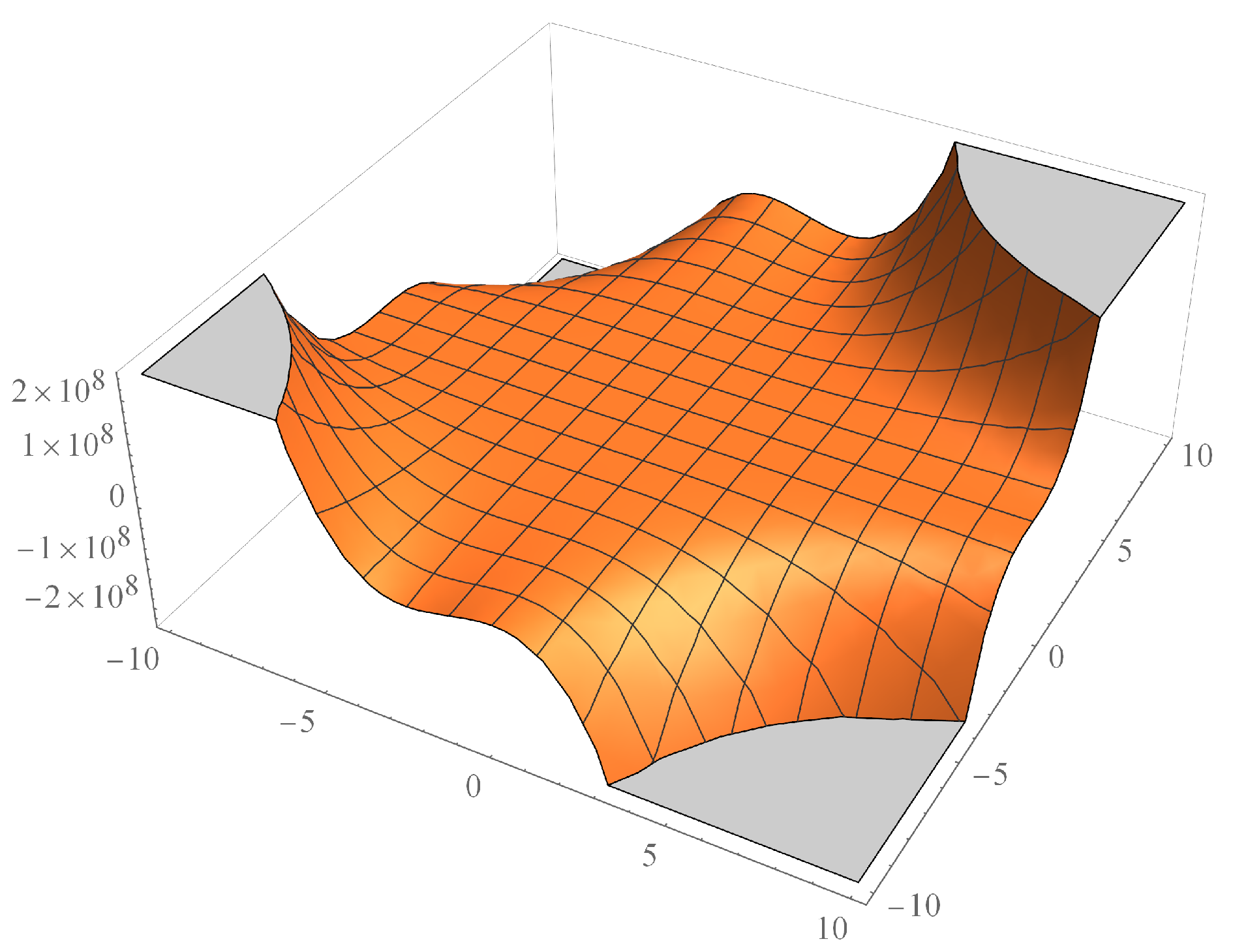
Now, we will give the 3D-plot of some of these M-polynomials with the help of Mathematica. In particulary, the 3d-plot of M-polynomial of dendrimer nanostar $N{D}_1\left[n\right]$ is shown in Figure 4 and for two nanotubes $G_3[n,m]$ and $G_4[n,m]$ in Figure 5 and Figure 6 respectively.

3.3. Degree-Based Topological Indices

In this subsection, by using the computed M-polynomials, some degree-based topological indices are determined for the aforementioned chemical graphs.

Theorem 7.

Let $G=N{D}_1\left[n\right]$. Then:

1 

$M_1(G)=204\times 2^{n-1}-78$

2 

$M_2(G)=246\times 2^{n-1}-99$

3 

${}^m{M}_2(G)=\frac{23}{3}\times 2^{n-1}-\frac{7}{3}$

4 

$R_{\alpha }(G)=4^{\alpha }(12\times 2^{n-1})+6^{\alpha }(24\times 2^{n-1}-12)+9^{\alpha }(6\times 2^{n-1}-3)$

5 

$R_{\alpha }(G)=\frac{1}{4^{\alpha }}(12\times 2^{n-1})+\frac{1}{6^{\alpha }}(24\times 2^{n-1}-12)+\frac{1}{9^{\alpha }}(6\times 26n-1-3)$

6 

$SDD(G)=88\times 2^{n-1}-32$

Proof. 

If $g(x,y)=M(N{D}_1\left[n\right],x,y)=(12\times 2^{n-1})x^2{y}^2+(24\times 2^{n-1}-12)x^2{y}^3+(6\times 2^{n-1}-3)x^3{y}^3$, then:

$\begin{array}{cc}\hfill D_x(g(x,y))& =(24\times 2^{n-1})x^2{y}^2+(48\times 2^{n-1}-24)x^2{y}^3\hfill \\ & +(18\times 2^{n-1}-9)x^3{y}^3\hfill \\ \hfill D_y(g(x,y))& =(24\times 2^{n-1})x^2{y}^2+(72\times 2^{n-1}-36)x^2{y}^3\hfill \\ & +(18\times 2^{n-1}-9)x^3{y}^3\hfill \\ \hfill S_x(g(x,y))& =(6\times 2^{n-1})x^2{y}^2+(12\times 2^{n-1}-6)x^2{y}^3\hfill \\ & +(2\times 2^{n-1}-1)x^3{y}^3\hfill \\ \hfill S_y(g(x,y))& =(6\times 2^{n-1})x^2{y}^2+(8\times 2^{n-1}-4)x^2{y}^3\hfill \\ & +(2\times 2^{n-1}-1)x^3{y}^3\hfill \end{array}$

$\begin{array}{cc}\hfill D_x{D}_y(g(x,y))& =(48\times 2^{n-1})x^2{y}^2+(144\times 2^{n-1}-72)x^2{y}^3\hfill \\ & +(54\times 2^{n-1}-27)x^3{y}^3\hfill \\ \hfill S_x{S}_y(g(x,y))& =(3\times 2^{n-1})x^2{y}^2+(4\times 2^{n-1}-2)x^2{y}^3\hfill \\ & +(\frac{2}{3}\times 2^{n-1}-\frac{1}{3})x^3{y}^3\hfill \\ \hfill D_x{S}_y(g(x,y))& =(12\times 2^{n-1})x^2{y}^2+(16\times 2^{n-1}-8)x^2{y}^3\hfill \\ & +(6\times 2^{n-1}-3)x^2{y}^3\hfill \\ \hfill D_y{S}_x(g(x,y))& =(12\times 2^{n-1})x^2{y}^2+(36\times 2^{n-1}-18)x^2{y}^3\hfill \\ & +(6\times 2^{n-1}-3)x^2{y}^3\hfill \end{array}$

$\begin{array}{cc}\hfill D_y^{\alpha }(g(x,y))& =2^{\alpha }(12\times 2n-1)x^2{y}^2+3^{\alpha }(24\times 2^{n-1}-9)x^2{y}^3\hfill \\ & +3^{\alpha }(6\times 2^{n-1}-3)x^3{y}^3\hfill \\ \hfill S_y^{\alpha }(g(x,y))& =\frac{1}{2^{\alpha }}(12\times 2n-1)x^2{y}^2+\frac{1}{3^{\alpha }}(24\times 2^{n-1}-9)x^2{y}^3\hfill \\ & +\frac{1}{3^{\alpha }}(6\times 2^{n-1}-3)x^3{y}^3\hfill \end{array}$

$\begin{array}{cc}\hfill D_x^{\alpha }{D}_y^{\alpha }(g(x,y))& =4^{\alpha }(12\times 2n-1)x^2{y}^2+6^{\alpha }(24\times 2^{n-1}-9)x^2{y}^3\hfill \\ & +9^{\alpha }(6\times 2^{n-1}-3)x^3{y}^3\hfill \\ \hfill S_x^{\alpha }{S}_y^{\alpha }(g(x,y))& =\frac{1}{4^{\alpha }}(12\times 2n-1)x^2{y}^2+\frac{1}{6^{\alpha }}(24\times 2^{n-1}-9)x^2{y}^3\hfill \\ & +\frac{1}{9^{\alpha }}(6\times 2^{n-1}-3)x^3{y}^3\hfill \end{array}$

Using the results above and substituting:

$$\begin{array}{cc}\hfill M_1(G)& =[(D_x+D_y){(g(x,y)]}_{(x,y)=(1,1)}=204\times 2^{n-1}-78\hfill \\ \hfill M_2(G)& ={\left[(D_x{D}_y)(g(x,y))\right]}_{(x,y)=(1,1)}=246\times 2^{n-1}-99\hfill \\ \hfill {}^m{M}_2(G)& ={\left[(S_x{S}_y)(g(x,y))\right]}_{(x,y)=(1,1)}=\frac{23}{3}\times 2^{n-1}-\frac{7}{3}\hfill \\ \hfill R_{\alpha }(G)& ={\left[(D_x^{\alpha }{D}_y^{\alpha })(g(x,y))\right]}_{(x,y)=(1,1)}=4^{\alpha }(12\times 2^{n-1})+6^{\alpha }(24\times 2^{n-1}-12)\hfill \\ & +9^{\alpha }(6\times 26n-1-3)\hfill \\ \hfill R_{\alpha }(G)& ={\left[(S_x^{\alpha }{S}_y^{\alpha })(g(x,y))\right]}_{(x,y)=(1,1)}=\frac{1}{4^{\alpha }}(12\times 2^{n-1})+\frac{1}{6^{\alpha }}(24\times 2^{n-1}-12)\hfill \\ & +\frac{1}{9^{\alpha }}(6\times 26n-1-3)\hfill \\ \hfill SDD(G)& ={\left[(D_x{S}_y+D_y{S}_x)(g(x,y))\right]}_{(x,y)=(1,1)}=88\times {22}^{n-1}-32\hfill \end{array}$$

 □

Theorem 8.

Let $G=N{D}_2\left[n\right]$. Then:

1 

$M_1(G)=680\times 2^n-622$

2 

$M_2(G)=836\times 2^n-771$

3 

${}^m{M}_2(G)=26\times 2^n-\frac{209}{9}$

4 

$R_{\alpha }(G)=(4^{\alpha }\times 56+6^{\alpha }\times 48+9^{\alpha }\times 36)\times 2^n-(4^{\alpha }\times 48+6^{\alpha }\times 44+9^{\alpha }\times 35)$

5 

$R_{\alpha }(G)=(\frac{1}{4^{\alpha }}\times 56+\frac{1}{6^{\alpha }}\times 48+\frac{1}{9^{\alpha }}\times 36)\times 2^n-(\frac{1}{4^{\alpha }}\times 48+\frac{1}{6^{\alpha }}\times 44+\frac{1}{9^{\alpha }}\times 35)$

6 

$SDD(G)=196\times 2^n-\frac{535}{3}$

Proof. 

If $g(x,y)=M(N{D}_2\left[n\right],x,y)=(56\times 2^n-48)x^2{y}^2+(48\times 2^n-44)x^2{y}^3+(36\times 2^n-35)x^3{y}^3$, then:

$$\begin{array}{cc}\hfill D_x{D}_y(g(x,y))& =4(56\times 2^n-48)x^2{y}^2+6(48\times 2^n-44)x^2{y}^3+9(36\times 2^n-35)x^3{y}^3\hfill \\ \hfill S_x{S}_y(g(x,y))& =\frac{1}{4}(6\times 2^{n-1})x^2{y}^2+\frac{1}{6}(8\times 2^{n-1}-4)x^2{y}^3+\frac{1}{9}(2\times 2^{n-1}-1)x^3{y}^3\hfill \\ \hfill D_x{S}_y(g(x,y))& =(56\times 2^n-48)x^2{y}^2+\frac{2}{3}(48\times 2^n-44)x^2{y}^3+(36\times 2^n-35)x^3{y}^3\hfill \\ \hfill D_y{S}_x(g(x,y))& =(56\times 2^n-48)x^2{y}^2+\frac{3}{2}(48\times 2^n-44)x^2{y}^3+(36\times 2^n-35)x^3{y}^3\hfill \\ \hfill D_x^{\alpha }{D}_y^{\alpha }(g(x,y))& =4^{\alpha }\times (56\times 2^n-48)x^2{y}^2+6^{\alpha }\times (48\times 2^n-44)x^2{y}^3\hfill \\ & +9^{\alpha }\times (36\times 2^n-35)x^3{y}^3\hfill \\ \hfill S_x^{\alpha }{S}_y^{\alpha }(g(x,y))& =\frac{1}{4^{\alpha }}(56\times 2^n-48)x^2{y}^2+\frac{1}{6^{\alpha }}(48\times 2^n-44)x^2{y}^3\hfill \\ & +\frac{1}{9^{\alpha }}(36\times 2^n-35)x^3{y}^3.\hfill \end{array}$$

Using the results above:

$$\begin{array}{cc}\hfill M_1(G)& ={\left[(D_x+D_y)(g(x,y))\right]}_{(x,y)=(1,1)}=680\times 2^n-622\hfill \\ \hfill M_2(G)& ={\left[(D_x{D}_y)(g(x,y))\right]}_{(x,y)=(1,1)}=836\times 2^n-771\hfill \\ \hfill {}^m{M}_2(G)& ={\left[(S_x{S}_y)(g(x,y))\right]}_{(x,y)=(1,1)}=26\times 2^n-\frac{209}{9}\hfill \\ \hfill R_{\alpha }(G)& ={\left[(D_x^{\alpha }{D}_y^{\alpha })(g(x,y))\right]}_{(x,y)=(1,1)}=(4^{\alpha }\times 56+6^{\alpha }\times 48+9^{\alpha }\times 36)\times 2^n\hfill \\ & -(4^{\alpha }\times 48+6^{\alpha }\times 44+9^{\alpha }\times 35)\hfill \\ \hfill R_{\alpha }(G)& ={\left[(S_x^{\alpha }{S}_y^{\alpha })(g(x,y))\right]}_{(x,y)=(1,1)}=(\frac{1}{4^{\alpha }}\times 56+\frac{1}{6^{\alpha }}\times 48+\frac{1}{9^{\alpha }}\times 36)\times 2^n\hfill \\ & -(\frac{1}{4^{\alpha }}\times 48+\frac{1}{6^{\alpha }}\times 44+\frac{1}{9^{\alpha }}\times 35)\hfill \\ \hfill SDD(G)& ={\left[(D_x{S}_y+D_y{S}_x)(g(x,y))\right]}_{(x,y)=(1,1)}=196\times 2^n-\frac{535}{3}\hfill \end{array}$$

 □

Theorem 9.

Let $G=G_1[n,m]$. Then:

1 

$M_1(G)=9mn-5m$

2 

$M_2(G)=\frac{27}{2}mn-\frac{21}{2}m$

3 

${}^m{M}_2(G)=\frac{1}{3}m+\frac{m}{18}(3n-5)$

4 

$R_{\alpha }(G)=6^{\alpha }\times 2m+9^{\alpha }(\frac{1}{2}m(3n-5))$

5 

$R_{\alpha }(G)=\frac{1}{6^{\alpha }}\times 2m+\frac{1}{9^{\alpha }}(\frac{1}{2}m(3n-5))$

6 

$SDD(G)=\frac{13}{3}m+m(3n-5)$

Proof. 

If $g(x,y)=M(G_1[n,m],x,y)=2m{x}^2{y}^3+(\frac{m}{2}(3n-5))x^3{y}^3$, then:

$\begin{array}{cc}\hfill D_x(g(x,y))& =4m{x}^2{y}^3+\frac{3}{2}m(3n-5)x^3{y}^3\hfill \\ \hfill D_y(g(x,y))& =6m{x}^2{y}^3+\frac{3}{2}m(3n-5)x^3{y}^3\hfill \\ \hfill S_x(g(x,y))& =m{x}^2{y}^3+\frac{m}{6}(3n-5)x^3{y}^3\hfill \\ \hfill S_y(g(x,y))& =\frac{2m}{3}{x}^2{y}^3+\frac{m}{6}(3n-5)x^3{y}^3\hfill \end{array}$

$\begin{array}{cc}\hfill D_x{D}_y(g(x,y))& =12m{x}^2{y}^3+\frac{9}{2}m(3n-5)x^3{y}^3\hfill \\ \hfill S_x{S}_y(g(x,y))& =\frac{m}{3}{x}^2{y}^3+\frac{m}{18}(3n-5)x^3{y}^3\hfill \\ \hfill D_x{S}_y(g(x,y))& =\frac{4}{3}m{x}^2{y}^3+\frac{m}{2}(3n-5)x^3{y}^3\hfill \\ \hfill D_y{S}_x(g(x,y))& =3m{x}^2{y}^2+\frac{m}{2}(3n-5)x^3{y}^3\hfill \end{array}$

$\begin{array}{cc}\hfill D_y^{\alpha }(g(x,y))& =3^{\alpha }\times 2m{x}^2{y}^3+3^{\alpha }(\frac{m}{2}(3n-5))x^3{y}^3\hfill \\ \hfill S_y^{\alpha }(g(x,y))& =\frac{1}{3^{\alpha }}\times 2m{x}^2{y}^3+\frac{1}{3^{\alpha }}(\frac{m}{2}(3n-5))x^3{y}^3\hfill \end{array}$

$\begin{array}{cc}\hfill D_x^{\alpha }{D}_y^{\alpha }(g(x,y))& =6^{\alpha }\times 2m{x}^2{y}^3+9^{\alpha }(\frac{m}{2}(3n-5))x^3{y}^3\hfill \\ \hfill S_x^{\alpha }{S}_y^{\alpha }(g(x,y))& =\frac{1}{6^{\alpha }}\times 2m{x}^2{y}^3+\frac{1}{9^{\alpha }}(\frac{m}{2}(3n-5))x^3{y}^3\hfill \end{array}$

Using the results above:

$$\begin{array}{cc}\hfill M_1(G)& ={\left[(D_x+D_y)(g(x,y))\right]}_{(x,y)=(1,1)}=9mn-5m\hfill \\ \hfill M_2(G)& ={\left[(D_x{D}_y)(g(x,y))\right]}_{(x,y)=(1,1)}=\frac{27}{2}mn-\frac{21}{2}m\hfill \\ \hfill {}^m{M}_2(G)& ={\left[(S_x{S}_y)(g(x,y))\right]}_{(x,y)=(1,1)}=\frac{1}{3}m+\frac{m}{18}(3n-5)\hfill \\ \hfill R_{\alpha }(G)& ={\left[(D_x^{\alpha }{D}_y^{\alpha })(g(x,y))\right]}_{(x,y)=(1,1)}=6^{\alpha }\times 2m+9^{\alpha }(\frac{1}{2}m(3n-5))\hfill \\ \hfill R_{\alpha }(G)& ={\left[(S_x^{\alpha }{S}_y^{\alpha })(g(x,y))\right]}_{(x,y)=(1,1)}=\frac{1}{6^{\alpha }}\times 2m+\frac{1}{9^{\alpha }}(\frac{1}{2}m(3n-5))\hfill \\ \hfill SDD(G)& ={\left[(D_x{S}_y+D_y{S}_x)(g(x,y))\right]}_{(x,y)=(1,1)}=\frac{13}{3}m+m(3n-5)\hfill \end{array}$$

 □

Theorem 10.

Let $G=G_2[n,m]$. Then:

1 

$M_1(G)=9mn-10m$

2 

$M_2(G)=\frac{27}{2}mn-20m$

3 

${}^m{M}_2(G)=\frac{1}{6}mn+\frac{5}{36}m$

4 

$R_{\alpha }(G)=4^{\alpha }\times m+6^{\alpha }\times 2m+9^{\alpha }\frac{1}{2}(m)(3n-8)$

5 

$R_{\alpha }(G)=\frac{1}{4^{\alpha }}\times m+\frac{1}{6^{\alpha }}\times 2m+\frac{1}{9^{\alpha }}\frac{1}{2}(m)(3n-8)$

6 

$SDD(G)=\frac{25}{6}m+m(3n-8)$

Proof. 

If $g(x,y)=M(G_2[n,m],x,y)=m{x}^2{y}^2+2m{x}^2{y}^3+(\frac{m}{2}(3n-8))x^3{y}^3$m then:

$$\begin{array}{cc}\hfill D_x{D}_y(g(x,y))& =4m{x}^2{y}^2+12m{x}^2{y}^3+\frac{9}{2}m(3n-8)x^3{y}^3\hfill \\ \hfill S_x{S}_y(g(x,y))& =\frac{1}{4}{x}^2{y}^2+\frac{1}{3}m{x}^2{y}^3+\frac{1}{18}m(3n-8)x^3{y}^3\hfill \\ \hfill D_x{S}_y(g(x,y))& =m{x}^2{y}^2+\frac{4}{3}m{x}^2{y}^3+\frac{1}{2}m(3n-8)x^3{y}^3\hfill \\ \hfill D_y{S}_x(g(x,y))& =m{x}^2{y}^2+3m{x}^2{y}^3+\frac{1}{2}m(3n-8)x^3{y}^3\hfill \\ \hfill D_x^{\alpha }{D}_y^{\alpha }(g(x,y))& =4^{\alpha }m{x}^2{y}^2+6^{\alpha }\times 2m{x}^2{y}^3+9^{\alpha }\times \frac{1}{2}m(3n-8)x^3{y}^3\hfill \\ \hfill S_x^{\alpha }{S}_y^{\alpha }(g(x,y))& =\frac{1}{4^{\alpha }}m{x}^2{y}^2+\frac{1}{6^{\alpha }}\times 2m{x}^2{y}^3+\frac{1}{9^{\alpha }}\times \frac{1}{2}m(3n-8)x^3{y}^3\hfill \end{array}$$

Using the results above:

$$\begin{array}{cc}\hfill M_1(G)& =9mn-10m\hfill \\ \hfill M_2(G)& =\frac{27}{2}mn-20m\hfill \\ \hfill {}^m{M}_2(G)& =\frac{1}{6}mn+\frac{5}{36}m\hfill \\ \hfill R_{\alpha }(G)& =4^{\alpha }\times m+6^{\alpha }\times 2m+9^{\alpha }\frac{1}{2}(m)(3n-8)\hfill \\ \hfill R_{\alpha }(G)& =\frac{1}{4^{\alpha }}\times m+\frac{1}{6^{\alpha }}\times 2m+\frac{1}{9^{\alpha }}\frac{1}{2}(m)(3n-8)\hfill \\ \hfill SDD(G)& =\frac{25}{6}m+m(3n-8)\hfill \end{array}$$

 □

Using the same proving arguments, we have the following theorems for the remaining two nanotubes $G=G_3[n,m]$ and $G=G_4[n,m]$.

Theorem 11.

Let $G=G_3[n,m]$. Then:

1 

$M_1(G)=36mn-40m$

2 

$M_2(G)=108mn-160m$

3 

${}^m{M}_2(G)=\frac{7}{24}m+\frac{1}{36}(3mn-8m)$

4 

$R_{\alpha }(G)={16}^{\alpha }\times 2m+{24}^{\alpha }\times 4m+{36}^{\alpha }\times (3mn-8m)$

5 

$R_{\alpha }(G)=\frac{1}{{16}^{\alpha }}\times 2m+\frac{1}{{24}^{\alpha }}\times 4m+\frac{1}{{36}^{\alpha }}\times (3mn-8m)$

6 

$SDD(G)=6mn-\frac{16}{3}m$

Theorem 12.

Let $G=G_4[n,m]$. Then:

1 

$M_1(G)=\frac{74}{3}mn-\frac{52}{3}m$

2 

$M_2(G)=65mn-\frac{208}{3}m$

3 

${}^m{M}_2(G)=\frac{19}{225}mn+\frac{133}{1800}m$

4 

$R_{\alpha }(G)=({30}^{\alpha }+{25}^{\alpha })mn+({16}^{\alpha }+\frac{8}{3}\times {20}^{\alpha }+\frac{4}{3}\times {24}^{\alpha }-\frac{8}{3}\times {25}^{\alpha }+4\times {30}^{\alpha })m$

5 

$R_{\alpha }(G)=(\frac{1}{{30}^{\alpha }}+\frac{1}{{25}^{\alpha }})mn+(\frac{1}{{16}^{\alpha }}+\frac{8}{3}\times \frac{1}{{20}^{\alpha }}+\frac{4}{3}\times \frac{1}{{24}^{\alpha }}-\frac{8}{3}\times \frac{1}{{25}^{\alpha }}+4\times \frac{1}{{30}^{\alpha }})m$

6 

$SDD(G)=\frac{212}{45}mn-\frac{10}{9}m$

4. Discussions

Topological indices are a numerical quantity computed from the molecular graph of a chemical compound and typically remain the same under graph isomorphism. They can be used to predict and model certain properties of chemical compounds; therefore, knowing the indices for these molecular graphs, we then understand the properties such as the chemical reactivity, physical features, biological activities, etc., of the associated molecule.

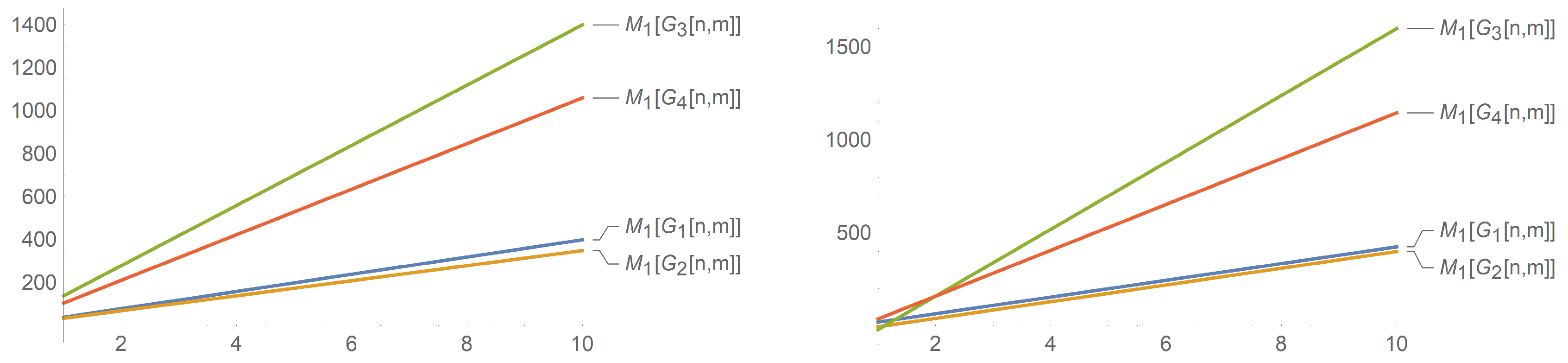
Having verified through experiments that the first Zagreb index is related to the total $\pi$-electron energy of the structure [18,19], hence a molecular graph having large values of $M_1\left[G\right]$ has a larger total $\pi$ electron energy. Following from Figure 7, we can find that both $N{D}_1\left[n\right]$ and $N{D}_2\left[n\right]$ have sharply rising total $\pi$-electron energy as values of n increase and that $N{D}_2\left[n\right]$ has a higher total $\pi$-electron energy as compared to $N{D}_1\left[n\right]$. Similarly, it follows from Figure 8 that the total $\pi$-electron energy of $G_3[n,m]$ is greater than the other three nanotubes for $m\ge 2$. It can also be observed that for a fixed value of m, the total $\pi$-electron energies of $G_1[n,m]$ and $G_2[n,m]$ only differ from each other by some constant value.

Likewise, from the general Randic index, we can obtain the Randic index proposed by Randic by replacing $\alpha$ with −0.5. It has been observed by the chemist Randic in 1975 that the Randic index can be used in determining the physiochemical properties of alkanes; he observed that there is a good correlation between the Randic index and some physio-chemical properties of alkanes: boiling points, chromatography retention times, enthalpies of formation, surface areas, etc. In reference to Figure 7, we could find that the Randic index of $N{D}_2\left[n\right]$ and $N{D}_1\left[n\right]$ both sharply increase with n and that $N{D}_2\left[n\right]$ is much greater than $N{D}_1\left[n\right]$. Observing Figure 9, we find that $G_1[n,m]=G_3[n,m]=G_2[n,m]$ for $\alpha =-0.5$. The Randic index for $G_4[n,m]$ is greater than the rest of the three nanotubes if $n\le 12$, and the three nanotubes have Randic indices that steadily increase past $G_4[n,m]$ for all $n>12$.

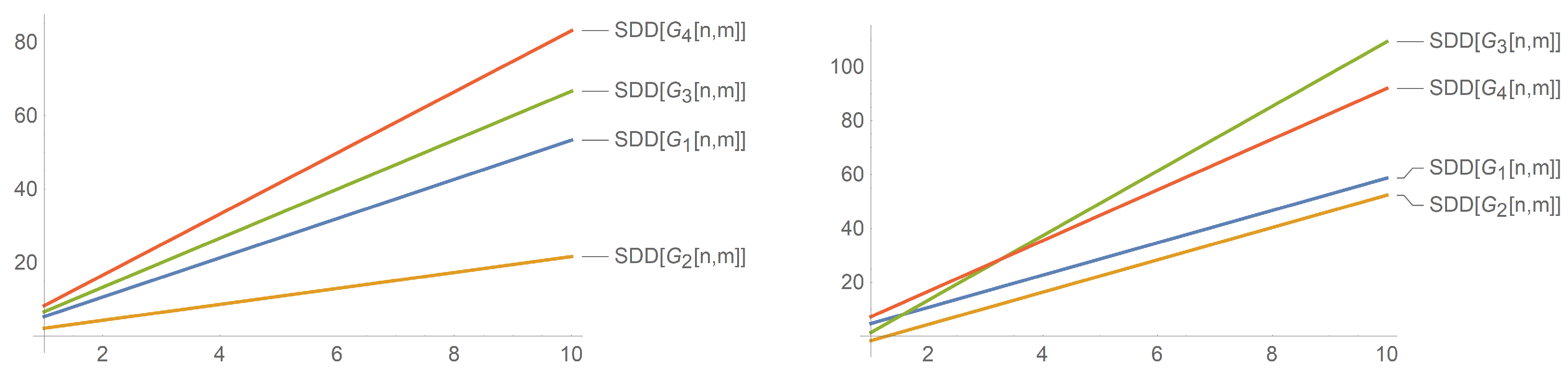
On the testing sets supplied by the International Academy of Mathematical Chemistry, it showed good predictive properties. It can also decently predict the total surface area for polychlorobiphenyls. Therefore, from Figure 8, we note that the symmetric division index of $N{D}_2\left[n\right]$$N{D}_1\left[n\right]$ rises sharply with $N{D}_2[n,m]$ being much greater than $N{D}_1[n,m]$. Similarly, we can also take note in reference to Figure 10 that $G_3[n,m]$ has the largest index among all four nanotubes for $n\ge 4$.

The above graphs for the nanotubes $G_k[n,m]$ show a correlation of $M_1\left[G\right]$, $R_{\alpha }\left[G\right]$, and $SDD\left[G\right]$ with n and m. It can be seen that the indices have a linear correlation with n and m. This contrasts the correlation of the indices of $D_1\left[n\right]$ and $N{D}_2\left[n\right]$ with n as the graphs are exponential and quickly rise. We only give an analysis for these three indices as the other indices ($M_2\left[G\right]$ and ${}^m{M}_2\left[G\right]$) are similar and can be obtained from the Randic index with specific values of $\alpha$ ($\alpha =1$ and $\alpha =-1$, respectively), and therefore, the correlation between the indices and n (and m) does not change.

5. Conclusions

We computed the M-polynomial of two classes of nanostar dendrimers and four nanotubes and used the M-polynomials to obtain a wide list of indices for our molecular graphs. By analyzing our results, we found that $N{D}_2\left[n\right]$ were better at achieving larger values of the calculated topological indices in comparison to $N{D}_1\left[n\right]$ and likewise that $G_3[n,m]$ were better at achieving larger values of these indices than the other three nanotubes. For future prospects, one can compute the M-polynomial for other types of nanostar dendrimers or nanotubes. For example, single-walled inorganic aluminosilicate and aluminogermanate nanotubes of a periodic structure and precise dimensions can be investigated related to the current study.

References

1. Basak, S.C. Use of graph invariants in quantitative structure-activity relationship studies. Croat. Chem. Acta 2016, 89, 419–429. [Google Scholar] [CrossRef]
2. Balaban, A.T. Can topological indices transmit information on properties but not on structures? J. Comput. Aided Mol. Des. 2005, 19, 651–660. [Google Scholar] [CrossRef] [PubMed]
3. Balaban, A.T. Chemical graph theory and the Sherlock Holmes principle. HYLE Int. J. Philos. Chem. 2013, 19, 107–134. [Google Scholar]
4. Ivanciuc, O. Chemical graphs, molecular matrices and topological indices in chemoinformatics and quantitative structure activity relationships. Curr. Comput. Aided Drug. Des. 2013, 9, 153–163. [Google Scholar] [CrossRef] [PubMed]
5. Emeric, D.; Sandi, K. M-polynomial revisited: Bethe cacti and an extension of Gutman’s approach. J. Appl. Math. Comput. 2019, 60, 253–264. [Google Scholar]
6. Klavzar, S.; Deutsch, E. M-polynomial and degree-based topological indices. Iran. J. Math. Chem. 2015, 6, 93–102. [Google Scholar]
7. Munir, M.; Nazeer, W.; Rafque, S.; Kang, S.M. M-polynomial and related topological indices of nanostar dendrimers. Symmetry 2016, 8, 97. [Google Scholar] [CrossRef]
8. Munir, M.; Nazeer, W.; Rafque, S.; Nizami, A.R.; Kang, S.M. M-polynomial and degree-based topological indices of titania nanotubes. Symmetry 2016, 8, 117. [Google Scholar] [CrossRef] [Green Version]
9. Munir, M.; Nazeer, W.; Rafque, S.; Kang, S.M. M-polynomial and degree-based topological indices of polyhex nanotubes. Symmetry 2016, 8, 149. [Google Scholar] [CrossRef] [Green Version]
10. Munir, M.; Nazeer, W.; Shahzadi, S.; Kang, S.M. Some invariants of circulant graphs. Symmetry 2016, 8, 134. [Google Scholar] [CrossRef] [Green Version]
11. Siddiqui, M.K.; Imran, M.; Ali, A. On Zagreb indices, Zagreb polynomials of some nanostar dendrimers. Appl. Math. Comput. 2016, 280, 132–139. [Google Scholar] [CrossRef]
12. Kulli, V.R. General fifth M-Zagreb indices and fifth M-Zagreb polynomials of PAMAM dendrimers. Int. J. Fuzzy Math. Arch. 2017, 13, 99–103. [Google Scholar]
13. Li, D.X.; Liu, J.B.; Farahani, M.R.; Rezaei, M. Zagreb indices and Zagreb polynomials of an infinite class of dendrimer nanostars. J. Comput. Theor. Nanosci. 2016, 13, 9136–9139. [Google Scholar] [CrossRef]
14. Kulli, V.R. Certain topological indices and their polynomials of dendrimer nanostars. Ann. Pure Appl. Math. 2017, 14, 263–268. [Google Scholar] [CrossRef]
15. Gao, W.; Younas, M.; Farooq, A.; Virk, A.U.R.; Nazeer, W. Some reverse degree-based topological indices and polynomials of dendrimers. Mathematics 2018, 6, 214. [Google Scholar] [CrossRef] [Green Version]
16. Yang, H.; Baig, A.Q.; Khalid, W.; Farahani, M.R.; Zhang, X. M-polynomial and topological indices of benzene ring embedded in P-type surface network. J. Chem. 2019, 2019, 7297253. [Google Scholar] [CrossRef]
17. Gutman, I.; Furtula, B.; Vukicevic, Z.K.; Popivoda, G. On Zagreb indices and coindices. MATCH Commun. Math. Comput. Chem. 2015, 74, 5–16. [Google Scholar]
18. Gutman, I.; Das, K.C. The first Zagreb index 30 years after. MATCH Commun. Math. Comput. Chem. 2004, 50, 83–92. [Google Scholar]
19. Nikolic, S.; Kovacvic, G.; Milicvic, A.; Trinajstic, N. The Zagreb indices 30 years after. Croat. Chem. Acta 2003, 76, 113–124. [Google Scholar]
Figure 1. (A) Molecular graph of N D 1 [ 2 ] ; (B) molecular graph of N D 2 [ 2 ] .
Symmetry 12 00831 g001
Figure 2. (A) Molecular graph of G 1 [ n , m ] ; (B) molecular graph of G 2 [ n , m ] .
Symmetry 12 00831 g002
Figure 3. (A) Molecular graph of G 3 [ n , m ] ; (B) molecular graph of G 4 [ n , m ] .
Symmetry 12 00831 g003
Figure 4. M-polynomial of N D 1 [ n ] for n = 10.
Symmetry 12 00831 g004
Figure 5. M-polynomial of G 3 [ n , m ] for n = 10 & m = 10.
Symmetry 12 00831 g005
Figure 6. M-polynomial of G 4 [ n , m ] for n = 10 & m = 10.
Symmetry 12 00831 g006
Figure 7. Comparison of some of the indices of N D 1 [ n ] , D 2 [ n ] for n = 0,...,10.
Symmetry 12 00831 g007
Figure 8. Comparison of the first Zagreb index of the nanotubes G k [ n , m ] .
Symmetry 12 00831 g008
Figure 9. Comparison of the Randic index of the nanotubes G k [ n , m ] and α = −0.5.
Symmetry 12 00831 g009
Figure 10. Comparison of the symmetric division index of the nanotubes G k [ n , m ] .
Symmetry 12 00831 g010