Abstract
This paper is devoted to developing a new computational method for nearly singular integral computation in the application of the boundary element method for the analysis of thin-shell-like structures in mechanical engineering. Based on the traditional distance transformation method, a sigmoidal transformation method is introduced to further cluster the integral points around the source point with respect to the circumferential direction. The combined method provides accurate results without employing a large quantity of integral points. Numerical examples demonstrate that the computational accuracy and efficiency of the proposed method is significantly higher than that of the traditional single distance transformation method, especially in the case of the asymmetric integral patch.
1. Introduction
In many implementations of the boundary element method (BEM) for analysis of mechanical problems, such as heat conductivity or elasticities on thin-shell-like structures [1,2], cracks [3,4,5], and punch forming of thin plates or shells [6,7,8], a large number of nearly singular integrals are involved and should be accurately computed with high efficiency. Similar numerical problems can also be found in some boundary meshfree approaches and peridynamic methods in which some singular basis functions are usually introduced to approximate the singularity [9,10]. The corresponding nearly singular integral is usually expressed as the following expression:
where means the distance between the field point x and the source point y in physical space, and represents the integral patch or element. The power l is usually considered as the order of the singularity. The integral in Equation (1) is regular if the source point y is located outside the integral patch. The integral becomes singular when the source point is located inside the integral patch. Many classic numerical quadrature formulas, including the well-known Gaussian quadrature formula and the Newton–Cotes quadrature formula, could be applied to accurately compute the regular integral.
However, the near-singularity arises when the source point approaches the integral patch. In this case, the regular integral becomes nearly singular. In the nearly singular integral, the integrand varies sharply in the integral region near the source point. Traditional numerical quadrature methods are usually theoretically based on the rational polynomial interpolation. The direct applications of those traditional numerical quadrature methods cannot provide results with satisfactory accuracy in the computation of the nearly singular integral [11].
In direct applications of traditional quadrature methods, high-ordered integral formulas or a large quantity of integral points are inevitably involved to accurately calculate the integral with a rapidly varying integrand [12]. Efforts are usually focused on how to adaptively subdivide the integral patches to achieve more accurate results while employing fewer integral points [13,14].
To further improve the accuracy of the computation without loss of efficiency, nonlinear transformations are usually performed before the implementation of the traditional quadrature scheme. Within the nonlinear transformations, a Jacobian term is generated in the integral to eliminate the singularity of the integrand. Several nonlinear transformations, such as the sinh transformation [15,16,17], the distance transformation [18,19], the polar coordinate transformation [20], the angular transformation [1,21], and the sigmoidal transformation [22,23], have been proposed to compute the nearly singular integral with a different singular order and over different types of integral elements.
All of these nonlinear transformations, however, are performed only in the radial direction in the integral space. In the case that the source point is located close to the boundary of the integral patch or that the integral patch is not symmetric to the source point, it has been found that the near-singularity not only arises in the radial direction but also in the circumferential direction [24]. The bidirectional nonlinear transformation is a natural choice for this problem.
The distance transformation was firstly applied by Ma in the computation of the nearly singular integral [18]. This transformation is the most efficient to weaken the radial directional near-singularity. Through the distance transformation, these integral points could be rearranged and clustered near the source point.
The sigmoidal transformation was first introduced by Johnson for computation of the nearly singular integral in 2D BEM applications [23]. Both the distance transformation and the sigmoidal transformation were originally applied in 2D BEM applications in which the boundary integral was defined over 1D segments. In 3D BEM, however, the boundary integral is usually performed over the boundary surfaces or patches. Based on the distance transformation, this paper performs the sigmoidal transformation in the circumferential variable to cluster the integral points towards the source point. Two numerical examples considering two differently ordered, nearly singular integrals will be presented to illustrate the validity and accuracy of the proposed scheme.
2. Statement of the Problem
In Figure 1, is the rectangular integral patch. xp represents the nearest point in the patch to the source point y. np denotes the out-normal of xp. The integrand in 3D BEM is usually of the following form:
in which is called the order of the singularity of the fundamental solution. is a smooth function. We are concerned with the case in which the source point y is located very close to the patch. The traditional Gaussian quadrature method usually leads to unacceptable results in the computation of the nearly singular integral.
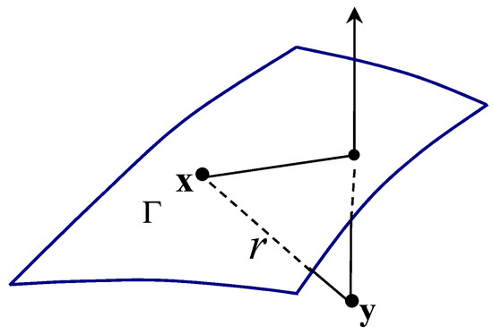
Figure 1.
The distance r from the source point y to an integral point x.
3. The Distance Transformation and the Sigmoidal Transformation
Before introduction of the distance transformation, the distance function in the parametric space should be defined. The components of the distance variable are usually rewritten parametrically as
In Equation (3), the components of the distance between the field point x and the center xp as defined in the introduction are expanded into the Taylor series. The superscript p denotes variables related to the center xp. The subscripts i and k denote the components in physical space. , represent the two parametric coordinates of x in space.
Before application of the distance transformation, the following polar transformation from to should be performed:
In space, the new form of Equation (3) is
in which is some function of but not related to . The distance between y and x can be expressed in space as
and further
In Equation (7), and
Considering the transformation in Equation (4), the integral in Equation (2) in space is
in which is the transformation Jacobian from the physical space to space. The function is the transformation Jacobian from the physical space to space.
3.1. The Distance Transformation
In space, we can define a distant function as introduced in [16]
With the definition of the distance function, the following distance transformation, which is of the exponential type, from to a new variable , can be constructed:
After applying Equation (10) to Equation (8), the integral in this newly constructed space has the following formulation:
3.2. The Sigmoidal Transformation
In Equation (11), the integral regarding the variable of seems to be regular if the order of the singularity is lower than 2. It has been observed that the integral regarding the variable may be also nearly singular in the case that the nearest point xp is located very closely to the boundary of the integral patch. To further eliminate this near-singularity, we introduce a sigmoidal transformation for that the variable .
The expression of sigmoidal transformation is of the following form:
The derivative is
This sigmoidal transformation, as illustrated in Equation (12), can cluster integration points in the interval (0,1) more closely to 0 and to 1.
4. Numerical Examples
To illustrate the accuracy of the presented method, two numerical examples considering two different ordered singular integrands, namely, and , are presented in this section. In each example, four teams of source points, for a total of 16 different source points, are employed to test the computational accuracy of the presented method and the compared method. Figure 2 illustrates the locations of the source point.
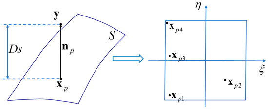
Figure 2.
Locations of source points.
The four parametric coordinates of the nearest points are , , , and . Four source points are distributed along the ray from each nearest point towards the direction of the normal . The distances, Ds, between the source points and the corresponding nearest points are , , , and . A is the area of the integral patch S. In all computations, 25 Gaussian quadrature points in the final integral space are employed for the numerical quadrature.
4.1. Numerical Integral With Integrand
This example concerns the effects of the presented bidirectional nonlinear transformation on the accuracy of the numerical integration. In this example, the following integral is computed by the presented method:
The integral patch S can be described as (−1, 1) × (−1, 1).
The results obtained by the presented method are compared with the reference results, which are obtained by a subdivision method with thousands of integral points. The results are also compared with the results obtained by the single distance transformation method. Table 1 lists the computational results with four different source points, for which the parametric coordinate of the corresponding nearest point is (−0.9, −0.9).

Table 1.
Results for the case of the nearest point (−0.9, −0.9) and the integrand .
The number in the round bracket is the relative error. In this case, the nearest point is located close to one corner of the integral square. It can be seen clearly from Table 1 that the accuracy of the presented method is higher than that of the singular distance transformation method by about three orders of magnitude. Table 2 lists the results for another four source points. The parametric coordinate of the corresponding nearest point is (−0.5, 0.5).
Table 2.
Results for the case of the second nearest point (−0.5, 0.5) and the integrand .
In this case, the nearest point is located in the center region of the integral square. It can be seen clearly from Table 2 that both methods can achieve very high accuracy. Table 3 illustrates the results in the case in which the parametric coordinate of the nearest point is (−0.9, 0.1).
Table 3.
Results for the case of the third nearest point (−0.9, 0.1) and the integrand .
A similar conclusion to that of the first case can be made in this comparison study. The presented method outperforms the single transformation method in terms of computational accuracy by about three orders of magnitude. Table 4 contains the results in the case in which the parametric coordinate of the nearest point is (−0.98, 0.9).
Table 4.
Results for the case of the fourth nearest point (−0.98, 0.9) and the integrand .
In this case, the nearest point is very close to the vertex of the integral patch. Results in Table 4 illustrate that the presented method achieves high computational accuracy in this special case. The computational accuracy of the single transformation method, however, is much lower.
4.2. Numerical Integral With Integrand
This example considers the computation of the nearly singular integral with the integrand . The singularity of the integrand is one order higher than that in the first example. In other words, the value of the integrand varies more rapidly with the variation of the integral point than that in the first example. The integral patch and the source points in this example are both the same as those in the previous example.
Table 5 illustrates the results computed by the bidirectional transformation method in comparison with the single distance transformation method in the case in which the nearest point to the four source points of the integral patch has the parametric coordinates (−0.9, −0.9).
Table 5.
Results for the case of the nearest point (−0.9, −0.9) and the integrand .
As illustrated in the above table, both methods can achieve acceptable results with high accuracy in the computation of the nearly hypersingular integral. In this case, the bidirectional transformation method performs better than the single transformation method but not by a significant margin. Table 6 lists the result in the case in which the nearest point is located in the center region of the integral patch.
Table 6.
Results for the case of the second nearest point (−0.5, 0.5) and the integrand .
In this case, the results obtained by the two methods are very similar to each other. This demonstrates that the sigmoidal transformation does not improve the accuracy of the computation. The circumferential near singularity is not significant when the nearest point is located far from the boundaries of the integral patch. Table 7 lists the results in the case in which the nearest point is located near another boundary of the integral patch.
Table 7.
Results for the case of the second nearest point (−0.9, 0.1) and the integrand .
The nearest point in this case is near one edge of the integral patch in the parametric space. However, the accuracy of the two methods is very similar. This is because the nearest point is not very close to the boundary. Table 8 lists the results in the case in which the nearest point is closer to the boundary of the integral patch in the parametric space.
Table 8.
Results for the case of the second nearest point (−0.98, 0.9) and the integrand .
The improvement, which is ascribed to the sigmoidal transformation in the circumferential direction, seems to be more significant in Table 8. In this case, higher accuracy with up to two orders of magnitude can be achieved by the sigmoidal transformation in the circumferential direction.
In order to illustrate the efficiency of the presented method, we performed the computations 10,000 times. The times taken for both methods are listed in Table 9. Furthermore, the time taken for the element subdivision method, which was applied to compute the reference result, is also listed as a comparison.
Table 9.
Comparisons of time consumption in the computation of the nearly singular integral with integrand .
It can be clearly seen in Table 9 that the transformation methods consume significantly less time than the element subdivision method. The efficiency of the present method is the same as that of the single distance transformation method. However, the present method provides significantly more accurate results than the single distance transformation method. It can be concluded from a comparison of all the tables that the combination of the sigmoidal transformation and the distance transformation can improve the accuracy of the computation of the nearly singular integral, especially in the case in which the source point is located near the boundary of the integral patch.
5. Conclusions
In this paper, the sigmoidal transformation and the distance transformation are combined to treat near-singularities in the boundary integral, which are common in BEM applications. In the combined transformation, the traditional distance transformation is performed for the radial variable in the integrand. The sigmoidal transformation is performed for the circumferential variable in the integrand. Two numerical examples are presented to validate the presented method. Numerical results illustrate the significant improvements, which are achieved by the combination of the sigmoidal transformation, in terms of computational accuracy.
Author Contributions
Methodology, writing-review and editing, supervision, project administration, funding acquisition, Z.L.; writing-original draft preparation, formal analysis, J.Y.; validation, funding acquisition, Q.Y.; data curation, software, F.Z.; All authors have read and agreed to the published version of the manuscript.
Funding
This research was funded by the Research and Development Planning Projects in Key Areas of Hunan Province (2019SK2174), the National Natural Science Foundation of China (11602082), Hunan Natural Science Foundation in China (2018JJ4059), and the scientific research fund of Hunan Provincial Education Department (19B145, 19C0577).
Conflicts of Interest
The authors declare no conflict of interest.
References
- Chen, S.; Liu, Y. A unified boundary element method for the analysis of sound and shell-like structure interactions. I. Formulation and verification. J. Acoust. Soc. Am. 1999, 106, 1247–1254. [Google Scholar] [CrossRef]
- Zhang, J.; Qin, X.; Han, X.; Li, G. A boundary face method for potential problems in three dimensions. Int. J. Numer. Methods Eng. 2009, 80, 320–337. [Google Scholar] [CrossRef]
- Xie, G.; Zhou, F.; Zhang, D.; Wen, X.; Li, H. A novel triangular boundary crack front element for 3D crack problems based on 8-node serendipity element. Eng. Anal. Bound. Elem. 2019, 105, 296–302. [Google Scholar] [CrossRef]
- Xie, G.; Zhou, F.; Li, H.; Wen, X.; Meng, F. A family of non-conforming crack front elements of quadrilateral and triangular types for 3D crack problems using the boundary element method. Front. Mech. Eng. 2019, 14, 332–341. [Google Scholar] [CrossRef]
- Feng, S.Z.; Han, X. A novel multi-grid based reanalysis approach for efficient prediction of fatigue crack propagation. Comput. Methods Appl. Mech. Eng. 2019, 353, 107–122. [Google Scholar] [CrossRef]
- Wei, Z.; Feng, J.; Ghalandari, M.; Maleki, A.; Abdelmalek, Z. Numerical Modeling of Sloshing Frequencies in Tanks with Structure Using New Presented DQM-BEM Technique. Symmetry 2020, 12, 655. [Google Scholar] [CrossRef]
- Zhang, J.; Shu, X.; Trevelyan, J.; Lin, W.; Chai, P. A solution approach for contact problems based on the dual interpolation boundary face method. Appl. Math. Model. 2019, 70, 643–658. [Google Scholar] [CrossRef]
- Shu, X.; Zhang, J.; Han, L.; Dong, Y. A surface-to-surface scheme for 3D contact problems by boundary face method. Eng. Anal. Bound. Elem. 2016, 70, 23–30. [Google Scholar] [CrossRef]
- Mossaiby, F.; Bazrpach, M.; Shojaei, A. Extending the method of exponential basis functions to problems with singularities. Eng. Comput. 2015, 32, 406–423. [Google Scholar] [CrossRef]
- Bazazzadeh, S.; Shojaei, A.; Zaccariotto, M.; Galvanetto, U. Application of the peridynamic differential operator to the solution of sloshing problems in tanks. Eng. Comput. 2019, 36, 45–83. [Google Scholar] [CrossRef]
- Qin, X.; Zhang, J.; Xie, G.; Zhou, F.; Li, G. A general algorithm for the numerical evaluation of nearly singular integrals on 3D boundary element. J. Comput. Appl. Math. 2011, 235, 4174–4186. [Google Scholar] [CrossRef]
- Wang, Q.; Zhou, W.; Cheng, Y.; Ma, G.; Chang, X. A line integration method for the treatment of 3D domain integrals and accelerated by the fast multipole method in the BEM. Comput. Mech. 2016, 59, 1–14. [Google Scholar] [CrossRef]
- Zhang, J.M.; Chi, B.T.; Singh, K.M. A binary-tree element subdivision method for evaluation of nearly singular domain integrals with continuous or discontinuous kernel. J. Comput. Appl. Math. 2019, 362, 22–40. [Google Scholar] [CrossRef]
- Zhang, J.; Wang, P.; Lu, C.; Dong, Y. A spherical element subdivision method for the numerical evaluation of nearly singular integrals in 3D BEM. Eng. Comput. 2017, 34, 2074–2087. [Google Scholar] [CrossRef]
- Johnston, P.R.; Elliott, D. A sinh transformation for evaluating nearly singular boundary element integrals. Int. J. Numer. Methods Eng. 2005, 62, 564–578. [Google Scholar] [CrossRef]
- Johnston, B.M.; Johnston, P.R.; Elliott, D. A sinh transformation for evaluating two-dimensional nearly singular boundary element integrals. Int. J. Numer. Methods Eng. 2007, 69, 1460–1479. [Google Scholar] [CrossRef]
- Xie, G.; Zhang, D.; Zhang, J.; Meng, F.; Du, W.; Wen, X. Implementation of sinh method in integration space for boundary integrals with near singularity in potential problems. Front. Mech. Eng. 2016, 11, 412–422. [Google Scholar] [CrossRef]
- Ma, H.; Kamiya, N. Distance transformation for the numerical evaluation of near singular boundary integrals with various kernels in boundary element method. Eng. Anal. Bound. Elem. 2002, 26, 329–339. [Google Scholar] [CrossRef]
- Ma, H.; Kamiya, N. A general algorithm for the numerical evaluation of nearly singular boundary integrals of various orders for two-and three-dimensional elasticity. Comput. Mech. 2002, 29, 277–288. [Google Scholar] [CrossRef]
- Lv, J.H.; Jiao, Y.Y.; Feng, X.T.; Wriggers, P.; Zhuang, X.Y.; Rabczuk, T. A series of Duffy-distance transformation for integrating 2D and 3D vertex singularities. Int. J. Numer. Methods Eng. 2019, 118, 38–60. [Google Scholar] [CrossRef]
- Qin, X.; Zhang, J.; Li, G.; Sheng, X.; Song, Q.; Mu, D. An element implementation of the boundary face method for 3D potential problems. Eng. Anal. Bound. Elem. 2010, 34, 934–943. [Google Scholar] [CrossRef]
- Elliott, D. The Cruciform Crack Problem and Sigmoidal Transformations. Math. Methods Appl. Sci. 1997, 20, 121–132. [Google Scholar] [CrossRef]
- Johnston, P.R. Application of sigmoidal transformations to weakly singular and near-singular boundary element integrals. Int. J. Numer. Methods Eng. 1999, 45, 1333–1348. [Google Scholar] [CrossRef]
- Zhou, F.; Wang, W.; Xie, G.; Liao, H.; Cao, Y. The Distance-Sinh combined transformation for near-singularity cancelation based on the generalized Duffy normalization. Eng. Anal. Bound. Elem. 2019, 108, 108–114. [Google Scholar] [CrossRef]


© 2020 by the authors. Licensee MDPI, Basel, Switzerland. This article is an open access article distributed under the terms and conditions of the Creative Commons Attribution (CC BY) license (http://creativecommons.org/licenses/by/4.0/).