Abstract
Recently, X-ray pulsar-based navigation (XPNAV) as a significant navigation method has been widely used in deep space exploration. However, the accuracy of XPNAV is limited to the existence of the pulsar direction error. To improve the performance of XPNAV, we have proposed a novel algorithm named “the modified augmented state extended Kalman filter” (MASEKF). The algorithm considers the high-order terms of direction error and then adds a more precise direction error into state equation and measurement equation. In the simulation, by comparing the performance of MASEKF, EKF, and ASEKF at the same time, it is found that MASEKF has better performance in the accuracy and stability, and the results also demonstrate that MASEKF algorithm has faster convergence speed. This paper provides a strong reference for other improvements of algorithms towards direction error. The purpose of this study is to establish MASEKF and add the direction error into the measurement equation and the state equation, so as to realize the coordination and symmetry of the algorithm.
1. Introduction
Over the past decades, the Global Positioning System (GPS), a well-known navigation method, has been performing well in low Earth orbit (LEO) satellite navigation [1]. It provides users with real-time position and speed information. Unaffected by the weather, the positioning accuracy of the single machine is better than 10 m. The dominant application and high precision of GPS have strongly impressed people. However, the GPS signal is designed to transmit information toward the earth; the dominating advantage of GPS cannot be used well in in-depth space exploration. Thus, GPS cannot provide autonomous navigation information services for spacecraft flying in interstellar space [2]. To overcome the above defects, X-ray pulsar-based navigation (XPNAV) is emerged that can work well in solving deep space problems; it uses the X-ray emitted by pulsars in the universe, then obtains the precise information of spacecraft by measuring the Time-of-Arrival (TOA) of X-ray pulsar radiation signals [3]. In XPNAV, the X-ray detector is installed on the spacecraft, the radiated X-ray photons are detected by the pulsar, the photon arrival time is measured, and the pulsar image information is extracted. After the corresponding signal and data processing, the spacecraft determines some parameters, such as the orbit of navigation, time, and attitude. As a matter of fact, XPNAV has attracted plenty of attention around the world.
In the previous researches of XPNAV, a significant research achievement is realized by proposing a recursive extended Kalman filter algorithm (EKF). Through the application of EKF, the accuracy of spacecraft’s position error can be controlled within 100 m, and the accuracy of velocity error is around 10 mm/s [4]. On the basis of EKF algorithm, a novel algorithm named the suboptimal multiple fading extended Kalman filter (SMFEKF) is established subsequently, which can be up to 65.43% and 61.70% lower than that with EKF for position and velocity errors, respectively [5]. Similarly, there is another algorithm named the strong tracking extended Kalman filter (STEKF), which has introduced the fading, to dynamically adjust the gain matrix; it is sure that STEKF can overcome the EKF defects in filtering performance degradation caused by the more complex nonlinear navigation model due to uncertainty. Therefore, STEKF has higher valuation accuracy, numerical stability, and strong traceability than EKF [6]. Besides EKF, other nonlinear state estimators have been developed such as the unscented Kalman filter (UKF), which as one of the sigma point Kalman filters, avoids a derivative calculation and has a higher theoretic precision than EKF [7]. Through incorporating state constraints in the UKF, the strong robustness of UKF is verified, and the performance of the UKF estimates is better compared to that of the EKF in the convergence rate as well as in the long-term state estimation error [8]. On the principles of UKF, a augmented state unscented Kalman filter (ASUKF) is proposed by regarding the system bias as a slowly time-varying augmented state; the simulation confirms its effectiveness and reliability [9]. Furthermore, a novel approach of the modified strong tracking Kalman filter (STUKF) is designed, which had introduced a defined suboptimal fading factor based on the orthogonality principle of the innovation vectors in the framework of the UKF into the prediction covariance to adjust the Kalman gain matrix; the effectiveness of the STUKF is demonstrated in the simulation experiments [10]. Recently, a lot of novel algorithms have been developed quickly, an Adaptive Divided Difference Filter (ADDF) algorithm is introduced, which had optimized pulsar’s position vector error by maximizing the incident flux density recorded by the X-ray detector; its simulation results had revealed that the navigation performance of ADDF can be improved by 70% compared with that of UKF and DDF [11]. Then, with the awareness of a tiny direction error may cause a huge system bias in XPNAV [12], a pulse time difference of arrival (TDOA) technology is proposed with the consideration about direction error, which is conducted by measuring several spacecraft simultaneously. Although the accuracy of XPNAV can improve a lot, the huge complex work and expensive operation do constrain the use of TDOA [13]. Another flexible method is to introduce the norm of direction error, which is verified to have higher accuracy by conducting rigorous simulation experiment. However, this algorithm relies heavily on the initial state of system bias and usually accompanies with large amount of calculation [14].
In this paper, different from prior works of literatures, the source of error that caused low accuracy of XPNAV is discussed carefully, recognizing the system error caused by pulsar direction error in detail. If changes of the dynamic model and measurement model are viewed as slowly time-varying, then the right ascension and declination of pulsar’s motion can be measured accurately. When Very Long Baseline Interferometry (VLBI) is the primary source of direction error, assuming that direction error unchanged during the measurement time step; hence, it is feasible to get a specific formula of direction error [4,12,15]. With consideration of the high-order terms of direction error, a new algorithm named Modified Augmented State Extended Kalman Filter (MASEKF) is constructed; it can optimize the state equation and measurement equation by introducing the improved direction error, which can be regarded as an innovative attempt. Besides, it is worth noting that EKF is applied widely in engineering due to its fast calculation speed, and thus, EKF is selected as the filtering part of MASEKF. In the simulation, under three different initial conditions, the performance of MASEKF is compared with that of ASEKF and EKF at the same time.
2. Materials and Methods
2.1. Theory of Pulsar Direction Error
2.1.1. The Principle of XPNAV
XPNAV is well suited in dealing with deep space exploration problems, and pulsar used in navigation can emit X-ray photon signals. During the process of the propagation of the signal, X-ray detector on the spacecraft can capture the signal to measure the amount and the arriving time of photon [16,17]. Subsequently, epoch folding method is used (it is the process of counting the recorded photons by means of direct folding or rapid folding and finally, normalizing the photon number and obtaining the pulse contour) [18] to obtain the time of the pulsar arrival at the spacecraft, using a pulsar timing method to get the time of the pulsar arrival at the center of the solar system (SSB). Then, XPNAV can calculate corresponding time delay between and [19]. Additionally, the corresponding distance can be acquired, which is the difference between the distance from SSB to pulsar and the distance from spacecraft to the pulsar. In addition, in spite of the tiny changes of pulsars, during the simulation period, when the position of the pulsar and the spacecraft’s initial parameters have been determined, a recursive estimation model of spacecraft position and velocity can be established accurately [20,21]. The basic principle of XPNAV is shown in Figure 1.

Figure 1.
The principle of X-ray pulsar-based navigation (XPNAV) (the parameters and geometric diagrams used by XPNAV).
Following the above analysis, it can be found that and are two fundamental parameters that need to be determined at the beginning, which is usually calculated by the epoch folding method. Another primary parameter can be easily determined by . The result of the system error is not negligible for the positional accuracy of the spacecraft. Thus, the pulse time model can be modified as follows [4,9].
where is the time from the pulsar to the SSB, is the time from the pulsar to the spacecraft, is the speed of light, stands for the real direction vector of the pulsar, is the vector from SSB to spacecraft, represents the relative distance between the pulsar and the SSB, is the position vector of SSB relative to the center of the sun, is the gravitational constant, is the mass of the sun, and is the system bias caused by the direction error of the pulsar. On the right-hand side of the expression, the first item is the first-order Doppler delay, which is the propagation time from the detector to the SSB and the pulsar to the SSB. The second item is the annual parallax caused by the annual change in the earth orbit, which together with the first term are collectively referred to as Roemer delay, and the third item is Shapiro delay [22].
As is indicated in Figure 1, since GPS satellite is used in the simulation, the orbital dynamics model is required to establish under the Earth-centered inertial (ECI) reference frame. Thereby the relationship of the vector between spacecraft, earth centroid, and SSB can be expressed below.
where represents the vector from SSB to spacecraft, is the vector between the spacecraft and earth center of mass, and stands for the vector between SSB and earth center of mass, which is usually obtained by JPL ephemeris DE421.
2.1.2. Analysis of System Error
In the process of applying XPNAV, system error was produced by the following aspects: 1. direction error , in this paper, Roemer delay and Shapiro delay were the main source of direction error; 2. clock error caused by clock drift; 3. the error caused by ; and 4. position error caused by ephemeris. In general, the ephemeris error is time varying and changes slowly. However, the ephemeris error can increase by 0.25 m within 1 h, which should be taken into account seriously in XPNAV [23]. Among the above four common errors, the error caused by is tiny, that is because the distance between the pulsar and the SSB is quite large [14,24]. Clock error is another vital item that do affect the accuracy of navigation; in the subsequent discussion, its value and possible changed situation are carefully considered.
In the prior studies, the Time-Differenced method is often used to handle system error. However, due to the inaccuracy of the initial model and without the consideration of direction error, after applying the Time-Differenced method in the Mars probe and Jupiter detector, it is found that the position error can even reach to the level of kilometers. Besides, as a commonly used algorithm UKF, constructing sampling points is easy to diverge and always accompany with poor stability. Some existing methods could not deal with the existence of large system error well [25]. To research the system error more scientifically, the other error terms causing system error should be discussed in detail, and the corresponding algorithm should be optimized to meet the higher accuracy requirements.
is obtained by the difference on the right-side term of Equation (1). In the difference, the corresponding terms of the real direction vector are different from the terms of the estimated direction vector, and after the elimination of the terms independent of the direction vector, Equation (3) is obtained as below.
where is the estimated unit direction vector.
In Equation (3), many terms are defining , but it is found that most existing algorithms only consider the effect of the first term . In fact, all terms in should be considered seriously; thus, a simple calculation is conducted to get the magnitude of every item in Equation (3); the specific position in the orbit of the ARGOS vehicles was chosen at time = 2451538.96769266 JD, and the results were only valid for this specific location. The single source used in this analysis was the Crab Pulsar, along with its proper motion of and and a distance of 2 kpc [26]. A value of was selected as a representation of the elapsed time between the measured and the current time [18].
In Table 1, it can be seen that the value of the first term is quite larger than that of other terms, but that does not mean that the term with smaller value can be discarded casually; it is found that even the third term with the smallest value can produce a position error around 0.45 (). Therefore, all terms in need to be handled carefully. In order to capture the subtle changes produced by , the derivative of versus time is calculated as is shown below.

Table 1.
The calculated results.
In accordance with Equation (4), it can be found that plays a vital role in , , and is the pulsar direction error as well. is the earth rotation rate; due to the existence of direction error and the earth rotation, the accompanied deviation can be quite large. For example, if the pulsar direction error is , the maximum value of the earth rotation rate is closed to 30.3 and the maximum of deviation is approximate to [27]. Therefore, the algorithm towards the pulsar direction error should be optimized further.
2.1.3. Analysis of Direction Error
According to literature [27], the Taylor series expansion of direction error should be discussed. Taylor’s series expansion method is widely used in the above arguments, but its quadratic terms and other terms are usually ignored [28], which is a primary reason because of which the direction error cannot be mainly eliminated.
In this part, the right ascension angle and the real declination angle form the pulsar direction vector; direction vector is usually shown as . Let the estimated position be , then the pulsar direction error can be calculated using
Usually, the real pulsar direction vector is expressed as follows.
In the prior researches, the high order terms in are ignored consistently; only the first-order term is saved in the final algorithm. Its expression is usually shown as follows.
In this paper, the high-order expansion terms of direction error are processed further; the second-order term of the Taylor series is shown below.
Actually, the apparent differences between the previous methods and the proposed method need to be shown clearly. We introduced the measurement equation and the state equation into discussions because these two equations can reflect the differences between various ways straightly.
2.2. The Improved Algorithm of MASEKF
Extended Kalman filter (EKF) is an efficient recursive filter that estimates the state of a dynamic system based on a series of measurements. It performs the first-order linear truncation of Taylor expansion of the nonlinear function but ignores the remaining higher order terms. Therefore, EKF is applicable for the nonlinear system [29]. However, ignoring the high-order terms does affect the navigation accuracy. In order to overcome the above defect, ASEKF is proposed by considering the state noise and measurement noise in the augmented state.
In the XPNAV, based on the dynamic equation of spacecraft in the Earth-centered inertial, to construct the state equation and measurement equation, several specific states as the position and velocity of the probe are selected to occupy in the equation, thereby the ordinary state equation of ASEKF is calculated as follows [30].
where r = ( is the position vector of the spacecraft in ECI, , v = ( is the velocity vector of the spacecraft in ECI,is the norm of pulsar direction error, is the gravity of the earth, which can be viewed as a fixed constant. is the second-order harmonic coefficient and is the radius of the earth. are the higher-order perturbation terms, such as solar radiation pressure perturbation, etc., which can be regarded as zero-mean Gaussian white noise. are the process noises in the rate of , which are normally handled as zero-mean Gaussian white noise as well.
It can be found that EKF improves the accuracy of Kalman filtering, then the accuracy of EKF is improved further by ASEKF, whereas ASEKF algorithm is optimized by adding the direction error terms, which has already been widely used in navigation around the world [31,32]. To improve the accuracy of ASEKF further, the other high-order terms existed in direction error should be considered seriously.
2.2.1. The State Equation
In this paper, MASEKF was proposed to meet higher accuracy requirements, which took the high-order terms of direction error into account seriously. As is indicated in Equation (8), the direction error has been expanded in second-order terms by Taylor series. To get the expression of the state equation of MASEKF, the formation of direction error is changed as follows.
where is the right ascension angle, is the first-order differential of right ascension, is the second-order differential of right ascension, is the real declination angle, is the first-order differential of the real declination angle, and is the second-order of differential of the real declination angle.
Then, combining Equation (10), the state equation of MASEKF is subsequently obtained. It can be shown as follows.
where is the Jacobian matrix of the system, is the second-order harmonic coefficient, is the radius of the earth, is the gravity of the earth, stand for the change rate of the right ascension and declination of the first pulsar, indicate the change rate of the right ascension and declination of the second pulsar, and show the change rate of the right ascension and declination of the third pulsar, is the process noise, and both and are the zero-mean Gaussian white noise.
2.2.2. The Measurement Equation
The changes in velocity vector and position vector were both considered in the MASEKF algorithm. The measurement model is determined as follows.
where, is the number of the selected pulsars, and is the measurement noise.
By combining Equation (1) and Equation (12) in the meantime, the measurement equation can be subsequently determined, which is calculated as follows.
where is the right-hand side of Equation (13). When , let the second item and the third item on the right side of Equation (18) be high-order term. Then, Equation (18) can be transformed as follows.
where is the difference between and . Though the high-order term is of a rather small magnitude, in order to avoid the truncation error as much as possible, it still should be linearized subsequently.
In the process of th filter calculation, the magnitude of is roughly equal to that of , hence, the term is used to replace the term . Equation (19) can be rewritten as follows.
where stands for the second term in Equation (18) and stands for the third term in Equation (18); they can be expressed as
Since the position of spacecraft in BCRS (Barycentric Celestial Reference System) can be viewed as same as that of the earth in BCRS, compared with the spacecraft’s position, the changes of spacecraft’s velocity and position were quite small. Thus, it is reasonable to let part of be replaced by , then Equations (22) and (23) can be expressed as follows.
Subsequently, the second-order Taylor expansion to at time was carried out. In order to make the process of expansion convenient, some simplification is done as follows.
Consequently, combining Equations (21), (24)–(27), the observation equation can be determined as follows.
where
3. Results and Discussion
3.1. The Procedures of Simulation
In order to further discuss the effectiveness and performance of the proposed algorithm, EKF and ASEKF were also simulated at the same time, and then all simulation results were analyzed in detail. In this paper, the procedures of the simulation were divided into four parts as Figure 2.

Figure 2.
The procedures of simulation.
- 1.
- Preprocessing
The work of preprocessing should be completed initially, which includes obtaining the parameters of pulsar, spacecraft, etc. The required parameters were determined through some official websites, databases, and software. In particular, the data of the pulsar’s position and velocity is obtained in the Australia Telescope National Facility (ATNF). In this study, Pulsar Catalogue was used to generate observation data, which is viewed as the real position as well [14]. It is worth mentioning that the pulsar position used in different algorithms is the real pulsar position plus the set error. Meanwhile, the position vector from the earth center of mass to SSB was obtained from DE421; STK software provided the necessary information of probe, such as position and velocity.
- 2.
- Observation Simulation
The main work of this part was to obtain the proper pulsars used in later simulation; all pulsars’ parameters were inputted into Inter Visual Fortran 11. Generally speaking, the higher the signal frequency of the pulsar, the greater the radiation energy of the photon, the smaller the background radiation energy, the narrower the pulse width in the periodic contour, the larger the number of pulses, the larger the quality factor of the pulsar, and the higher the positioning accuracy of the pulsar. Under the constraints of positioning accuracy and quality factor, Weighted Dilution Of Precision (WDOP) method and observation analysis to acquire the most suitable pulsars were used [21]. Specifically, after selecting pulsars, the most important thing was to determine the time delay. The number of photons reaching the detector can be obtained by simulating the number of photons generated in Poisson distribution. The pulse profile of simulated observation can be obtained by adding the number of photons repeatedly. Then, using the FFT method to cross-correlate the simulated observation profile with the standard pulse profile, the time delay can be obtained in the end.
- 3.
- Analysis of System Error
In this research, the direction error caused by Roemer delay and Shapiro delay was analyzed in detail.
- 4.
- Orbit Determination
The core work involved in this part was conducted based on the MASEKF module, combining orbital dynamics to process the simulated observation data. The state of the spacecraft was obtained, and the precision statistics of the calculated results were carried out. When the precision evaluation exceeds the threshold value of Cramer-Rao Lower Bound [33], the simulation was finished, otherwise, the orbit simulation was simulated again. The experiment cannot stop simulating until the accuracy meets the requirements.
To make this research more comprehensive, the performance of three different algorithms was verified further. Root mean square error (RMSE) was applied to confirm the simulation precision of three algorithms, which can quantify the deviation between the observed values and real values straightly. It is worth noting that RMSE is extremely sensitive to outliers, such as maximum error and minimum error. The expression of RMSE is as follows.
where is the of the estimated position error, is the RMSE of the estimated velocity error, is the sampling point of the stable filter interval, is the estimated position error, is the initial moment of filtering stability, and is the estimated velocity error. In the end, of the three algorithms was calculated and analyzed cautiously.
3.2. Initial Conditions
Actually, there are 140 pulsars that can be used in navigation; in this paper, WDOP method was applied with the constraint of quality factor to select 40 pulsars, which is the process of preliminary selection as well. If the selected 40 pulsars have better performances, then the most suitable pulsars are chosen through observation analysis. Finally, three pulsars (B1821-24, B1937+21, and B0531+21) were adopted as the navigation sources. The corresponding parameters of the three pulsars are shown in Table 2.
Table 2.
Parameters of the pulsars.
In the simulation, the research object was the earth-orbiting spacecraft. The parameters are presented in Table 3. Meanwhile, it is well accepted that GPS plays a vital role in the navigation system, and its data is available [13,25]; many prior studies have selected GPS as the research object due to its importance and extensive application. Thus, GPS_BII-10 was adapted to be further researched in this paper; its corresponding data are provided by STK software. The simulation time was set between 2017.10.1.16.00.00 and 2017.10.2.16.00.00. The measurement time step was determined as 246.8 , whose effectiveness has been confirmed many times in the existing pieces of literature [3,19]. Usually, the filtering step runs immediately after the pulsar observation step [34]. The total time of the simulation was 86,400 ; the simulation parameters of EKF, ASEKF, and MASEKF were set as follows.
Table 3.
Parameters of the orbit.
- (1)
- Initial state error:
- (2)
- Initial estimation-error covariance:
- (3)
- The covariance of the state process noise:
In addition, the observation noise covariance can be determined as follows [18].
where, is the width of the pulsar, is the X-ray background radiation flux, which is about 0.005 in the prior researches, is the radiation photon flux from the pulsar, is the ratio of the pulse radiation flux to the average radiation flux in one pulsar period, is the effective area of the X-ray detector, its value is 1 , is the observation period, , and is the ratio of to .
The pulsar period parameters are shown in Table 2. Hence, the covariance of observation noise can be calculated. The result of is given by
where is an abbreviation for diagonal matrix.
3.3. Simulation and Analysis
In the simulation, in order to confirm the performance of the proposed algorithm clearly, ASEKF and EKF were simulated to be compared with MASEKF, conducting the simulation under three different conditions. In this paper, the factor of the direction error is an essential changeable condition of the simulation, since the system error includes the direction error, clock error, ephemeris error, and other possible existing errors, the settings of the above errors are presented below.
- 1.
- Clock error
The initial clock error, the clock error drift, and change rate of the drift were set as , 4.136679, and 6.88, respectively.
- 2.
- Ephemeris error
According to reference [35], the ephemeris error is usually less than in the other planets’ ephemerides. However, the error in the earth’s ephemeris has been verified to be the biggest, which could have specific influences on the performance of XPNAV. Since the simulation time is from 2017.10.1.16.00.00 to 2017.10.2.16.00.00, and ephemeris is time varying. Consequently, the changeable tendency of ephemeris error within the simulation period can be determined in Figure 3.

Figure 3.
The approximate ephemeris error in 2017.
- 3.
- Direction error
Owing to the limited space and the previous attempts in other works of literature [34], the simulation was conducted with the initial error condition of (0 mas, 0 mas), (1 mas, 1 mas), and (−1 mas, −1 mas); it should be noted that mas as a unit represents milli–arcsecond.
- 4.
- Cosmic background noise
In the observation and simulation stage, the photon arrival model under the Poisson distribution to simulate the distribution of cosmic background noise was construct; it was found that the pulse observation profile of the photon arrival model under the Poisson distribution was closest to the actual pulse profile. In the orbit determination stage, cosmic background noise was added to the observation noise, and then it was subjected to the Kalman filter algorithm for processing.
- 5.
- Other errors
According to the prior researches, other errors may mainly exist in the following aspects: (1) the distance between SSB and spacecraft, the greater the distance, the higher the system error; (2) the value of the pulsar frequency derivative, the larger the value, the larger the system error, and (3) the size of proper motion and the age of the position epoch, the greater the appropriate motion, the older the epoch, the greater the system error. Considering the above possible existing errors, other errors were set to .
Besides, the simulated observation data was combined with random noise. By adding the random noise during the simulation process of obtaining and , whose value is usually less than the corresponding position error can be controlled within 30 . Besides, the uncertainty information (the triple standard deviation) was added to prove the reliability of the estimated results. The data are indicated in Figure 4, Figure 5 and Figure 6.
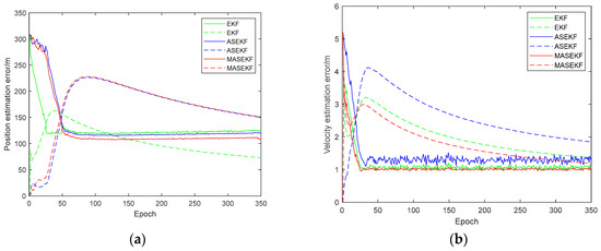
Figure 4.
The estimated result when the position error is (0 mas, 0 mas). (a) The estimated position error and (b) the estimated velocity error. The solid line represents the estimation results of different algorithms, and the dashed line represents the triple standard deviation of different algorithms.
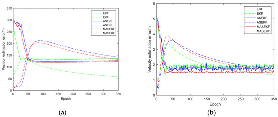
Figure 5.
The estimated result when the position error is (1 mas, 1 mas). (a) The estimated position error and (b) the estimated velocity error. The solid line represents the estimation results of different algorithms, and the dashed line represents the triple standard deviation of different algorithms.
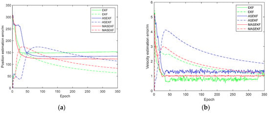
Figure 6.
The estimated result when the position error is (−1 mas, −1 mas). (a) The estimated position error and (b) the estimated velocity error. The solid line represents the estimation results of different algorithms, and the dashed line represents the triple standard deviation of different algorithms.
In Figure 4, Figure 5 and Figure 6, it can be found that the estimated result of the position error fluctuates greatly, especially in the case of (0 mas, 0 mas), the estimated result of EKF’s position error cannot satisfy the requirement of the triple standard deviation around 50 epochs, which indicates the poor performance of EKF. In contrast, the estimated results of ASEKF and MASEKF’s position error are acceptable in scenarios of (0 mas, 0 mas) and (1 mas, 1 mas), it is notable that the estimated result of velocity error of three algorithms can satisfy the requirement of the triple standard deviation, which can strongly illustrate the effectiveness of ASEKF and MASEKF under any simulation condition.
Table 4 displays the statistical simulation results, when there is no initial error; it is apparent that EKF has the worst performance. It is well accepted that EKF performs Kalman filtering by linearizing the nonlinear system, ignoring the direction error term unconsciously. This means that EKF cannot eliminate the corresponding measurement noise and state noise effectively; the above defects of EKF result in its lower accuracy. Through analyzing Figure 4, it was found that the velocity error of EKF diverges at 300~350 epochs, which was rather unstable, thereby it was tough for the system to converge on the whole.
Table 4.
The simulation results of the three algorithms.
What’s more, different from EKF algorithm, ASEKF algorithm linearizes the nonlinear system after adding the direction error into the state vector, considering the first-order term of the direction error in Taylor series expansion, which could certainly improve the accuracy in a way. Therefore, the accuracy of ASEKF has improved a lot than that of EKF, but the performance of ASEKF seems to be a little bit of unstable, as indicated in Figure 5 and Figure 6. It could be seen that the accuracy of ASEKF decreases quickly in scenarios of (−1 mas, −1 mas); the accuracy difference between (−1 mas, −1 mas) and (1 mas, 1 mas) is much bigger than that of between (0 mas, 0 mas) and (1 mas, 1 mas), and it seems that ASEKF is more suited in scenarios of (0 mas, 0 mas) and (1 mas, 1 mas).
Furthermore, based on the theory of the ASEKF algorithm, the proposed MASEKF has considered the second-order terms of direction error, adding the more accurate direction error into the state equation and measurement equation subsequently. Therefore, the MASEKF algorithm tends to have a better convergence effect and stronger stability. As is shown in Table 4, it is evident that MASEKF has the best accuracy performance under three different conditions; the accuracy of ASEKF is close to the accuracy of MASEKF in scenarios of (1 mas, 1 mas). Besides, MASEKF can converge quickly to 121 m in position error, whereas the velocity error of MASEKF converges rapidly to about 0.729 m/s after about 50 epochs. It seems that the improvement and optimization of MASEKF only bring a small increase in accuracy in scenarios of (1 mas, 1 mas). In fact, when the simulation are conducted in situations of (−1 mas, −1 mas), the advantages of MASEKF stand out, the accuracy of MASEKF is quite higher than the other two algorithms, and its accuracy difference is quite small between (−1 mas, −1 mas) and (1 mas, 1 mas), which verifies the better stability of MASEKF.
What’s more, for the purpose of comparing the performance of different algorithms further, simulations were conducted to obtain the RMSE under different conditions; RMSE can reflect the difference of the accuracy straightly. Figure 7, Figure 8 and Figure 9 show the performance comparison of EKF, ASEKF, and MASEKF under different initial conditions.
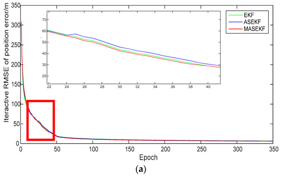
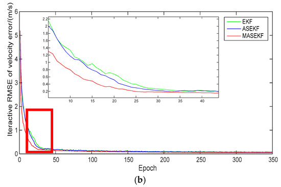
Figure 7.
Iterative root mean square error (RMSE) of three algorithms in scenarios of (0 mas, 0 mas). (a) Iterative RMSE of position error and (b) iterative RMSE of velocity error.
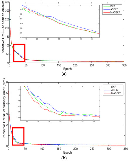
Figure 8.
Iterative RMSE of three algorithms in scenarios of (1 mas, 1 mas). (a) Iterative RMSE of position error and (b) iterative RMSE of velocity error.
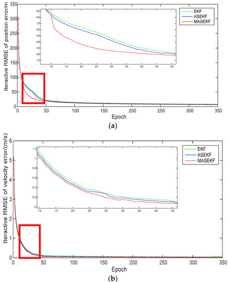
Figure 9.
Iterative RMSE of three algorithms in scenarios of (−1 mas, −1 mas). (a) Iterative RMSE of position error and (b) iterative RMSE of velocity error.
For clarity, Table 5 lists the necessary information of Figure 7, Figure 8 and Figure 9. Regardless of whether there was system bias, MASEKF always had the fastest converge speed and the best navigation accuracy. The performance of ASEKF was much better than that of EKF, which illustrated that the optimization of the high-order terms of the direction error significantly improved the accuracy of the algorithm. Besides, it can also be observed that the proposed algorithm considered second-order terms of Taylor series of direction error, which outperforms the algorithm that only considered the first-order terms of Taylor series of direction error. Furthermore, as is shown in Table 6, the accuracy of EKF and ASEKF was analyzed compared to that of MASEKF. It was found that EKF has poor accuracy, especially in scenarios of (0 mas, 0 mas), and the accuracy of the velocity error of MASEKF was improved by 43.06% than that of EKF. Similarly, the accuracy of the velocity error of MASEKF was improved by 36.11% than that of ASEKF. Meanwhile, though the accuracy of ASEKF improved a lot than the traditional EKF algorithm, its performance cannot stay stable in all conditions, such as in scenarios of (1 mas, 1 mas); the accuracy of position error and velocity error of ASEKF were worse than that of EKF. All values were positive in Table 6, which means that the accuracy of EKF and ASEKF were worse than that of MASEKF. In fact, MASEKF always performed well, compared with traditional EKF algorithm, and it increased the average accuracy by 8.84% and 20.53% in position error and velocity error, respectively, under the three conditions.
Table 5.
The results of root mean square error (RMSE) under different conditions.
Table 6.
The comparison performance of different algorithms with the modified augmented state extended Kalman filter (MASKEF).
To confirm the stability of the proposed algorithm in the whole simulation period, we compared the simulated orbit with the real one. The simulated trajectories and their partial enlargement are shown in Figure 10 [25]. It is evident that the MASEKF algorithm has the closest approximation between the simulated track and the real track at any simulation time. All results demonstrated that MASEKF not only had obvious superiority in the overall result but also ensured its high accuracy and stability at any time.
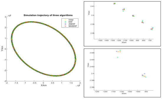
Figure 10.
Stability test of the algorithm.
4. Conclusions
In this paper, MASEKF algorithm is proposed based on the ASEKF algorithm, which expands the second-order term of the direction error to reduce the high-order truncation errors. Adding the more precise direction error into the state equation and measurement equation, thus, MASEKF can reduce the non-Gaussian error propagation in the nonlinear system. Finally, simulation is conducted by comparing the performance of MASEKF, ASEKF, and EKF. It is found that MASEKF is more versatile and efficient, compared with traditional EKF algorithm, and MASEKF can even increase the average accuracy by 8.84% and 20.53% in position error and velocity error, respectively, in the three simulation conditions. In the future, scholars can research the reliable algorithm of pulsar position error or other errors according to the algorithm proposed in this paper.
Author Contributions
L.L. has collected data and verified results. X.R. has proposed CIR algorithm along with other authors and given suggestions to improve the paper. G.N. has validated the results and provided fund support. All authors have read and agreed to the published version of the manuscript.
Funding
This research was funded by the National Natural Science Foundation Project of China (Grant No. 41074023).
Acknowledgments
We thank the helpful and important suggestions of the editors and reviewers.
Conflicts of Interest
The authors declare no conflicts of interest.
References
- Shen, L.-R.; Li, X.-P.; Sun, H.-F.; Fang, H.-Y.; Xue, M.-F. A robust compressed sensing based method for X-ray Pulsar Profile construction. Optik 2016, 127, 5542. [Google Scholar] [CrossRef]
- Xiong, K.; Wei, C.; Liu, L. Performance enhancement of X-ray pulsar navigation using autonomous optical sensor. Acta Astronaut. 2016, 128, 473–484. [Google Scholar] [CrossRef]
- Anderson, K.D.; Pines, D.J.; Sheikh, S.I. Validation of Pulsar Phase Tracking for Spacecraft Navigation. J. Guid. Control Dyn. 2015, 38, 1885–1897. [Google Scholar] [CrossRef]
- Xu, Q.; Wang, H.-L.; Feng, L.; You, S.-H.; He, Y.-Y. A novel X-ray pulsar integrated navigation method for ballistic aircraft. Optik 2018, 175, 28–38. [Google Scholar] [CrossRef]
- Du, J.; Fei, B.J.; Liu, Y.; Xiao, Y. Application of STEKF in X-ray Pulsar Based Autonomous Navigation. Int. Workshop Inf. Electron. Eng. 2012, 29, 4369–4373. [Google Scholar] [CrossRef][Green Version]
- Wan, E.A.; van der Merwe, R.; IEEE. The unscented Kalman Filter for nonlinear estimation. In Proceedings of the IEEE 2000 Adaptive Systems for Signal Processing, Communications, and Control Symposium 2000, Lake Louise, AB, Canada, 1–4 October 2000; pp. 153–158. [Google Scholar] [CrossRef]
- Kandepu, R.; Foss, B.; Imsland, L. Applying the unscented Kalman filter for nonlinear state estimation. J. Process Control 2008, 18, 753–768. [Google Scholar] [CrossRef]
- Liu, J.; Ma, J.; Tian, J.W.; Kang, Z.W.; White, P. X-ray pulsar navigation method for spacecraft with pulsar direction error. Adv. Space Res. 2010, 46, 1409–1417. [Google Scholar] [CrossRef]
- Liang, T.T.; Wang, M.; Zhou, Z.H. State Estimation for Sampled-Data Descriptor Nonlinear System: A Strong Tracking Unscented Kalman Filter Approach. Math. Probl. Eng. 2017, 2017, 5640309. [Google Scholar] [CrossRef]
- Zhang, H.; Jiao, R.; Xu, L.P. Orbit Determination Using Pulsar Timing Data and Orientation Vector. J. Navig. 2019, 72, 155–175. [Google Scholar] [CrossRef]
- Liu, J.; Ma, J.; Tian, J.W.; Kang, Z.W.; White, P. Pulsar navigation for interplanetary missions using CV model and ASUKF. Aerosp. Sci. Technol. 2012, 22, 19–23. [Google Scholar] [CrossRef]
- Zhang, H.; Jiao, R.; Xu, L.P.; Xu, C.Y.; Mi, P. Formation of a Satellite Navigation System Using X-Ray Pulsars. Publ. Astron. Soc. Pac. 2019, 131, 17. [Google Scholar] [CrossRef]
- Xu, Q.; Wang, H.L.; Feng, L.; Jiang, W.; You, S.H.; He, Y.Y. An improved augmented X-ray pulsar navigation algorithm based on the norm of pulsar direction error. Adv. Space Res. 2018, 62, 3187–3198. [Google Scholar] [CrossRef]
- Goshenmeskin, D.; Baritzhack, I.Y. Observability Analysis of Piece-Wise Constant Systems.2. Application to Inertial Navigation In-Flight Alignment. IEEE Trans. Aerosp. Electron. Syst. 1992, 28, 1068–1075. [Google Scholar] [CrossRef]
- Wei, E.; Jin, S.; Zhang, Q.; Liu, J.; Li, X.; Yan, W. Autonomous navigation of Mars probe using X-ray pulsars: Modeling and results. Adv. Space Res. 2013, 51, 849–857. [Google Scholar] [CrossRef]
- Lin, H.Y.; Xu, B.; Liu, J.X. Designing observation scheme in X-ray pulsar-based navigation with probability ellipsoid. Adv. Space Res. 2019, 64, 1639–1651. [Google Scholar] [CrossRef]
- Sheikh, S.I.; Pines, D.J.; Ray, P.S.; Wood, K.S.; Lovellette, M.N.; Wolff, M.T. The use of x-ray pulsars for spacecraft navigation. Adv. Astronaut. Sci. 2005, 119, 105–119. [Google Scholar]
- Sheikh, S.I.; Pines, D.J.; Ray, P.S.; Wood, K.S.; Lovellette, M.N.; Wolff, M.T. Spacecraft navigation using x-ray pulsars. J. Guid. Control Dyn. 2006, 29, 49–63. [Google Scholar] [CrossRef]
- Yu, W.H. Characterization of X-Ray Pulsar Navigation for Tracking Closed Earth Orbits. J. Guid. Control Dyn. 2019, 42, 2310–2313. [Google Scholar] [CrossRef]
- Zheng, S.J.; Zhang, S.N.; Lu, F.J.; Wang, W.B.; Gao, Y.; Li, T.P.; Song, L.M.; Ge, M.Y.; Han, D.W.; Chen, Y.; et al. In-orbit Demonstration of X-Ray Pulsar Navigation with the Insight-HXMT Satellite. Astrophys. J. Suppl. Ser. 2019, 244, 1. [Google Scholar] [CrossRef]
- Yu, W.H.; Inst, N. Application of X-Ray Pulsar Navigation: A Characterization of the Earth Orbit Trade Space. In Proceedings of the 29th International Technical Meeting of the Satellite Division of the Institute of Navigation, Portland, OR, USA, 12–16 September 2016; pp. 845–856. [Google Scholar]
- Archinal, B.A.; A′Hearn, M.F.; Bowell, E.; Conrad, A.; Consolmagno, G.J.; Courtin, R.; Fukushima, T.; Hestroffer, D.; Hilton, J.L.; Krasinsky, G.A.; et al. Report of the IAU Working Group on Cartographic Coordinates and Rotational Elements: 2009. Celest. Mech. Dyn. Astron. 2011, 109, 101–135. [Google Scholar] [CrossRef]
- Zhou, Y.; Wu, P.; Li, X. XANV/GNSS-Based Integrated Navigation Using a Robust Filtering Algorithm. J. Aeronaut. Astronaut. Aviat. 2016, 48, 123–131. [Google Scholar] [CrossRef]
- Gui, M.Z.; Ning, X.L.; Ma, X.; Zhang, J. A Novel Celestial Aided Time-Differenced Pulsar Navigation Method Against Ephemeris Error of Jupiter for Jupiter Exploration. IEEE Sens. J. 2019, 19, 1127–1134. [Google Scholar] [CrossRef]
- Caraveo, P.A.; Mignani, R.P. A new HST measurement of the Crab pulsar proper motion. Astron. Astrophys. 1999, 344, 367–370. [Google Scholar]
- Guo, P.B.; Sun, J.; Xue, J. X-ray pulsar navigation using multiple detectors based on a new observation strategy. IET Radar Sonar Navig. 2018, 12, 442–448. [Google Scholar] [CrossRef]
- Seidelmann, P.K.; Archinal, B.A.; A′Hearn, M.F.; Conrad, A.; Consolmagno, G.J.; Hestroffer, D.; Hilton, J.L.; Krasinsky, G.A.; Neumann, G.; Oberst, J.; et al. Report of the IAU/IAG Working Group on cartographic coordinates and rotational elements: 2006. Celest. Mech. Dyn. Astron. 2007, 98, 155–180. [Google Scholar] [CrossRef]
- Li, M.Z.; Xu, B. Autonomous orbit and attitude determination for Earth satellites using images of regular-shaped ground objects. Aerosp. Sci. Technol. 2018, 80, 192–202. [Google Scholar] [CrossRef]
- Scott, R.; Ploen, D.P.S.; Fred, Y.; Hadaegh, A.; Acikmese, B. Dynamics of Earth Orbiting Formations. Collect. Tech. Pap. Aiaa Guid. Navig. Control Conf. 2004. [Google Scholar] [CrossRef]
- Delva, P.; Kostić, U.; Čadež, A. Numerical modeling of a Global Navigation Satellite System in a general relativistic framework. Adv. Space Res. 2011, 47, 370–379. [Google Scholar] [CrossRef]
- Cui, P.; Wang, S.; Gao, A.; Yu, Z. X-ray pulsars/Doppler integrated navigation for Mars final approach. Adv. Space Res. 2016, 57, 1889–1900. [Google Scholar] [CrossRef]
- Batista, P. Long baseline navigation with explicit pseudo-range clock offset and propagation speed estimation. Eur. J. Control 2019, 49, 116–130. [Google Scholar] [CrossRef]
- Pines, J.; Ray, P.S.; Wood, K.S. Spacecraft Navigation Using X-Ray Pulsars. J. Guid. Control Dyn. 2006, 29. [Google Scholar] [CrossRef]
- Rong, J.; Luping, X.; Zhang, H.; Cong, L. Augmentation method of XPNAV in Mars orbit based on Phobos and Deimos observations. Adv. Space Res. 2016, 58, 1864–1878. [Google Scholar] [CrossRef]
- Wang, Y.; Zheng, W.; Sun, S.; Li, L. X-ray pulsar-based navigation system with the errors in the planetary ephemerides for Earth-orbiting satellite. Adv. Space Res. 2013, 51, 2394–2404. [Google Scholar] [CrossRef]


© 2020 by the authors. Licensee MDPI, Basel, Switzerland. This article is an open access article distributed under the terms and conditions of the Creative Commons Attribution (CC BY) license (http://creativecommons.org/licenses/by/4.0/).