Construction of Local Shape Adjustable Surfaces Using Quintic Trigonometric Bézier Curve

Abstract

Based on quintic trigonometric Bézier like basis functions, the biquintic Bézier surfaces are modeled with four shape parameters that not only possess the key properties of the traditional Bézier surface but also have exceptional shape adjustment. In order to construct Bézier like curves with shape parameters, we present a class of quintic trigonometric Bézier like basis functions, which is an extension of a traditional Bernstein basis. Then, according to these basis functions, we construct three different types of shape adjustable surfaces such as general surface, swept surface and swung surface. In addition to the application of the proposed method, we also discuss the shape adjustment of surfaces showing with curvature nephogram (with and without fixing the boundaries). However, the modeling examples shows that the suggested approach is efficient and easy to implement.

1. Introduction

In Computer Aided Geometric Design (CAGD) and Computer Graphics (CG), Bézier curves and surfaces are not only important for modeling free form curves and surfaces, but also useful in design and geometrically presenting different products. However, it has several limitations that restrict its applications in engineering, animation, automobile industries and other disciplines. For example, once control points are given, the position of the Bézier curves are fixed relative to their control polygon. Their shapes can only be modified by adjusting the control points. If users do not prefer to change the control points, the shape parameter curves or surfaces is a good choice.

To enhance the flexibility and gaining satisfying graphics, researchers have comes up with various kind of spline curves and surfaces with shape parameter. In recent years, many scholars have paid attention to the trigonometric Bézier curves. In [1,2], Bashir et al. presented quadratic and rational quadratic trigonometric Bézier curves with single and double shape parameters, respectively. Xiao-qin and Han [3] presented cubic trigonometric polynomial curves with two shape parameters that can deal preciously with circular arc, cones, cylinders and many more. Yan [4] discussed the cubic trigonometric nonuniform spline basis functions by proving their total positivity property. Han et al. [5] presented a cubic trigonometric Bézier curve with two shape parameters and managed to show the representation of ellipses using T-Bézier curves. The cubic trigonometric Bézier curves by [5] are being extended to construct spiral [6] and transition curves [7]. Dube and Sharma [8] presented a quartic trigonometric Bézier-like curve with one shape parameter and defined the corresponding trigonometric Bézier surfaces. Meanwhile, Han [9] presented piecewise quartic polynomial curves with a local shape parameter. The proposed curves can approximate an ellipse from both sides. Misro et al. [10] developed quintic trigonometric Bézier curve with two shape parameters. The proposed curve is later applied in constructing five templates of transition curves [11].

For the design of interpolation curves, Yan [12] constructed the trigonometric curves that can interpolate the specified data points automatically without solving equation schemes, which offer a simple and effective way of constructing interpolation curves, but these curves have only one degree of freedom. In extension to this, Li. [13] presents a new method of curve interpolation using cubic trigonometric interpolation curves with two shape parameters. This method also automatically interpolates the given data but have two degrees of freedom. Cao and Weng [14] introduce shape-adjustable non-uniform B-spline curves under the fixed control polygons as well as discussing some geometric properties of the curves. Misro et al. [15] used cubic trigonometric Bézier curves with two shape parameter and develop S-shaped and C-shaped transition curve by satisfying $G^2$ Hermite condition. Yang and Zeng [16] presented the Triangular Bézier curves and surface with n and $3n(n+1)/2$ shape change parameters, respectively, which simplified the work of Chenglin [17], giving one united expression of shape change parameter and by making the geometric significance clearer. Su and Tan [18], established quasi-cubic B-spline base curves and surface by trigonometric polynomials and shows the representation of straight lines, circular arcs, sine curves and sphere.

Moreover, Chand and Tyada [19] studied on the shape preserving while introducing the concept of using partially blended rational cubic trigonometric fractional interpolation surfaces. Xumin and Weixiang [20] developed method of free-form surface modeling and gave examples for its application to analyzed the effect of shape parameters over the surfaces. Hu et al. [21] studied the continuity conditions between generalized Bézier-like surfaces with multiple shape parameters and also discuss some properties and applications of the smooth continuity by providing the modeling examples. Lasser [22] proposed an algorithm for converting a rectangular patch of a triangular Bézier surface into a tensor product Bézier representation and also discuss the corner problem of a surface. The curves and surfaces in [1,2,3,4,5,6,7,8,9,10,18,19,20,21] have several specific advantages such as they inherit the positive properties of the classical Bézier curves and surfaces. Furthermore, several local shape parameters are included and make it possible to change the local shapes of the curves and surfaces without altering the control points. All these curves and surfaces are highly flexible and suitable in shape design where the shapes could be modified directly by the boundary curves, but they are non-interpolating on boundaries. In response to the existing approach, the paper aims to create local shape adjustable surfaces using a quintic trigonometric Bézier-like basis function with four shape parameters that not only possess the key properties of the classical Bézier surfaces but also have exceptional shape adjustment with and without fixing the boundary curves. Moreover, we examine the geometric continuity conditions of the two adjacent quintic trigonometric surfaces to make a smooth joint between surface patches and effect of shape parameters on surface using mean curvature nephogram are also provided. In conclusion, the applications to the surface modeling in engineering are explored together with Coons surfaces at fixed boundary curves.

The rest of the paper is organized as follows. The quintic trigonometeric Bézier basis function is defined in Section 2. The construction of Bézier surface with shape parameter is presented in Section 3. In Section 4, we propose the $G^2$ continuity conditions for biquintic trigonometric Bézier surfaces. Some examples of $G^2$ smooth continuity between two adjacent surfaces are given in Section 5. In Section 6 and Section 7, the discussion about swept and swung surfaces are given. In Section 8, the effect of shape parameter on shape adjustable surfaces showing with mean curvature nephogram is presented. Finally, conclusion and suggestions are provided in Section 9.

2. Quintic Trigonometric Bézier Basis Function

Quintic trigonometric Bézier curve with two shape parameters $\alpha$ and $\beta$ is defined in [10] as:

$$r\left(t\right)=\sum _{i=0}^5{P}_i{f}_i\left(t\right),$$

(1)

where $P_i\in R^m$ ($m=2,3$) is the control point located in plane or space and $f_i$ is the basis function for quintic trigonometric Bézier with $i=0,1,2,3,4,5$ whereas,

$$\left\{\begin{array}{c}\begin{array}{cc}\hfill f_0\left(t\right)& ={(1-sin\frac{\pi t}{2})}^4(1-\alpha sin\frac{\pi t}{2}),\hfill \\ \hfill f_1\left(t\right)& =sin\frac{\pi t}{2}{(1-sin\frac{\pi t}{2})}^3(4+\alpha -\alpha sin\frac{\pi t}{2}),\hfill \\ \hfill f_2\left(t\right)& ={(1-sin\frac{\pi t}{2})}^2(1-cos\frac{\pi t}{2})(8sin\frac{\pi t}{2}+3cos\frac{\pi t}{2}+9),\hfill \\ \hfill f_3\left(t\right)& ={(1-cos\frac{\pi t}{2})}^2(1-sin\frac{\pi t}{2})(8cos\frac{\pi t}{2}+3sin\frac{\pi t}{2}+9),\hfill \\ \hfill f_4\left(t\right)& =cos\frac{\pi t}{2}{(1-cos\frac{\pi t}{2})}^3(4+\beta -\beta cos\frac{\pi t}{2}),\hfill \\ \hfill f_5\left(t\right)& ={(1-cos\frac{\pi t}{2})}^4(1-\beta cos\frac{\pi t}{2})\hfill \end{array}\end{array}\right.$$

(2)

where $\alpha ,\beta$∈ [−4, 1] are shape parameters for the following six functions of t, where t∈ [0, 1].

Theorem 1.

Quintic trigonometric Bézier basis functions (2) have the following properties:

(a) 

Non-negativity: $f_i\left(t\right)\ge 0,i=0,1,2,3,4,5$

(b) 

Partition of unity: ${\sum }_{i=0}^5{f}_i\left(t\right)=1$

(c) 

Symmetry: $f_i(t,\alpha ,\beta )=f_{5-i}(1-t,\alpha ,\beta )$ for $i=[0,5]$

Proof. 

(a)

For $t\in [0,1]$ and $\alpha ,\beta$$\in [-4,1]$, then $1-sin\frac{\pi t}{2}\ge 0$, $1-cos\frac{\pi t}{2}\ge 0$,

$sin\frac{\pi t}{2}\ge 0$, $cos\frac{\pi t}{2}\ge 0$, $1-\alpha sin\frac{\pi t}{2}\ge 0,$$1-\beta cos\frac{\pi t}{2}\ge 0$,

$4+\alpha -\alpha sin\frac{\pi t}{2}\ge 0$, $4+\beta -\beta sin\frac{\pi t}{2}\ge 0$.

(b)

${\sum }_{i=0}^5{f}_i\left(t\right)=f_0\left(t\right)+f_1\left(t\right)+f_2\left(t\right)+f_3\left(t\right)+f_4\left(t\right)+f_5\left(t\right)=1$.

(c)

$\begin{array}{cc}\hfill f_0(t,\alpha ,\beta )& ={(1-sin\frac{\pi t}{2})}^4(1-\alpha sin\frac{\pi t}{2})\hfill \\ \hfill & ={(1-cos\frac{\pi (1-t)}{2})}^4(1-\beta cos\frac{\pi (1-t)}{2})\hfill \\ \hfill & =f_5(1-t,\beta ,\alpha )\hfill \end{array}$

 □

The quintic trigonometric Bézier basis function for two arbitrarily selected real values of shape parameters $\alpha$ and $\beta$ is shown in Figure 1.

3. Construction of Biquintic Trigonometric Bézier Surface with Shape Parameter

If the control points $P_{i,j}\in R^3(i=0,1,...m;j=0,1,...,n;m,n=5)$ are given, the parameteric surface

$$\begin{array}{cc}S(u,v;{\alpha }_1,{\beta }_1,{\alpha }_2,{\beta }_2)={\sum }_{i=0}^m{\sum }_{j=0}^n{f}_{i,m}\left(u\right)f_{j,n}\left(v\right)P_{i,j},& for(u,v)\in [0,1]\times [0,1]\end{array}$$

(3)

is called the tensor product biquintic trigonometric Bézier surface of degree m and n with ${\alpha }_1,{\beta }_1$ and ${\alpha }_2,{\beta }_2$ are the shape parameters of the basis functions $f_{i,m}\left(u\right)(i=0,1,...,m)$ and $f_{j,n}\left(v\right)(j=0,1,...,n)$, respectively as defined in Equation (2).

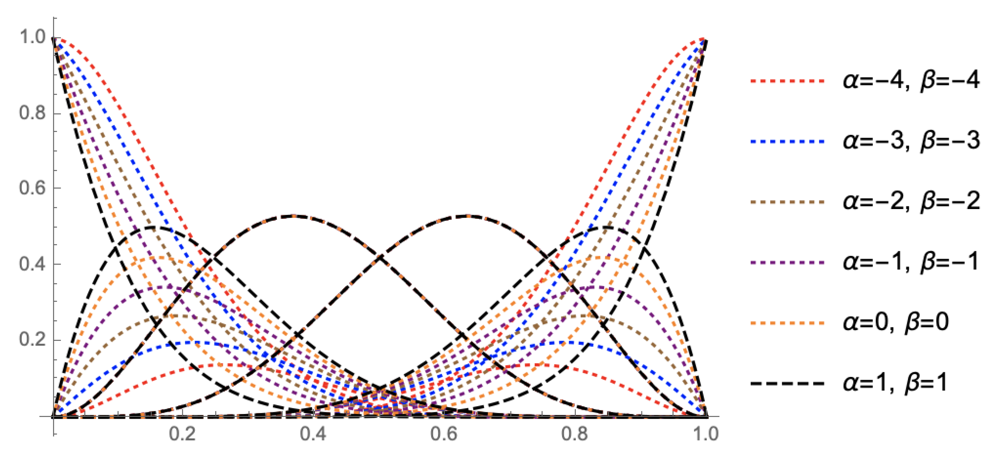
Remark 1.

Biquintic trigonometric Bézier surface with shape parameter in Equation (3) inherited most of the properties of classical Bézier surface including, boundary property, convex hull, symmetric and invariance.

Remark 2.

The shape of the surface in Equation (3) can be adjusted flexibly by changing the shape parameters subject to the condition that its control points remain unchanged.

Figure 2 shows biquintic trigonometric Bézier surface with different shape parameters values. In Figure 2, the biquintic trigonometric Bézier surfaces have 36 control points and 4 shape parameters ${\alpha }_1,{\beta }_1$ and ${\alpha }_2,{\beta }_2$. In Figure 2a–d, the values of shape parameter ${\alpha }_1$, ${\beta }_1$ and ${\alpha }_2$, ${\beta }_2$ are decreasing in the range of $[-4,1]$ which is changing in both the u-direction and v-direction. The biquintic trigonometric Bézier surface moves away from its control nets as shape parameter decreasing. Figure 2e,f displays the surfaces when changes are made only in the v-direction. The surface moves away from one side without affecting the other side when one shape parameter changes. However, shape parameters in the biquintic trigonometric Bézier surface provide the flexibility in surface modeling either in one or both directions.

4. G² Continuity Conditions for Biquintic Trigonometric Bézier Surfaces

In practical applications, various kinds of complex surfaces are encountered. In designing the complex surfaces, designers usually have to achieve $G^1$ continuity on adjacent surfaces. However, in situations with high demand for smoothness, $G^2$ continuity is also required, that is, surfaces need to have a common tangent plane at any point on their common boundary. Suppose that there are two biquintic trigonometric Bézier surfaces needed to satisfy $G^2$ smooth continuity:

$$\left\{\begin{array}{c}\begin{array}{c}\hfill S_1(u,v;{\alpha }_1,{\beta }_1,{\alpha }_2,{\beta }_2)=\sum _{i=0}^{m_1}\sum _{j=0}^{n_1}{f}_{i,m_1}(u;{\alpha }_1,{\beta }_1)f_{j,n_1}(v;{\alpha }_2,{\beta }_2)P_{i,j}^1\\ \hfill S_2(u,v;{\alpha }_1^{*},{\beta }_1^{*},{\alpha }_2^{*},{\beta }_2^{*})=\sum _{i=0}^{m_2}\sum _{j=0}^{n_2}{f}_{i,m_2}(u;{\alpha }_1^{*},{\beta }_1^{*})f_{j,n_2}(v;{\alpha }_2^{*},{\beta }_2^{*})P_{i,j}^2.\end{array}\end{array}\right.$$

(4)

where $-4\le {\alpha }_1,{\beta }_1,{\alpha }_2,{\beta }_2,{\alpha }_1^{*},{\beta }_1^{*},{\alpha }_2^{*},{\beta }_2^{*}\le 1$, $P_{i,j}^1$ $(i=0,1,...,m_1=5;j=0,1,...,n_1=5)$ and $P_{i,j}^2$ $(i=0,1,...,m_2=5;j=0,1,...,n_2=5)$ are control points of the surfaces $S_1(u,v;{\alpha }_1,{\beta }_1,{\alpha }_2,{\beta }_2)$ and $S_2(u,v;{\alpha }_1^{*},{\beta }_1^{*},{\alpha }_2^{*},{\beta }_2^{*})$, respectively. Surfaces are different from curves due to the directivity, so there exists continuity in three types of directions namely the u-direction, u- and v-directions and v-direction.

4.1. Continuity in the u Direction

In order to achieve $G^2$ continuity between two surfaces of $S_1(u,v;{\alpha }_1,{\beta }_1,{\alpha }_2,{\beta }_2)$ and $S_2(u,v;{\alpha }_1^{*},{\beta }_1^{*},{\alpha }_2^{*},{\beta }_2^{*})$ in the u-direction, the surfaces are required to achieve $G^0$ and $G^1$ continuity at a joint point [23,24]. Let $S_1(u,v;{\alpha }_1,{\beta }_1,{\alpha }_2,{\beta }_2)$ and $S_2(u,v;{\alpha }_1^{*},{\beta }_1^{*},{\alpha }_2^{*},{\beta }_2^{*})$ be two surfaces in the u-direction. The surfaces will achieve $G^0$ when

$$S_1(u,1;{\alpha }_1,{\beta }_1,{\alpha }_2,{\beta }_2)=S_2(u,0;{\alpha }_1^{*},{\beta }_1^{*},{\alpha }_2^{*},{\beta }_2^{*})$$

(5)

which results in

$$\sum _{i=0}^{m_1}{f}_{i,m_1}(u;{\alpha }_1,{\beta }_1)P_{i,n_1}^1=\sum _{i=0}^{m_2}{f}_{i,m_2}(u;{\alpha }_1^{*},{\beta }_1^{*})P_{i,0}^2.$$

(6)

The Equation (6) can be simplified by comparing the coefficients, $m_1=m_2$, ${\alpha }_1={\alpha }_1^{*}$, ${\beta }_1={\beta }_1^{*}$, as follows:

$$P_{i,n_1}^1=P_{i,0}^2.$$

(7)

By definition of the $G^1$ smooth continuity, the two surfaces are required to have a continuous tangential derivative across the boundary. Therefore, they need to satisfy the following conditions:

$$\begin{array}{c}\frac{\partial }{\partial v}{S}_1(u,1;{\alpha }_1,{\beta }_1,{\alpha }_2,{\beta }_2)\times \frac{\partial }{\partial u}{S}_1(u,1;{\alpha }_1,{\beta }_1,{\alpha }_2,{\beta }_2)\hfill \\ \hfill =\varphi \left(u\right)\frac{\partial }{\partial v}{S}_2(u,0;{\alpha }_1^{*},{\beta }_1^{*},{\alpha }_2^{*},{\beta }_2^{*})\times \frac{\partial }{\partial u}{S}_2(u,0;{\alpha }_1^{*},{\beta }_1^{*},{\alpha }_2^{*},{\beta }_2^{*})\end{array}$$

(8)

where $\varphi \left(u\right)$ is a scaling vector between the normal vector such that $\varphi \left(u\right)>0$. The simplified form of Equation (8) can be written as:

$$\frac{\partial }{\partial v}{S}_1(u,1;{\alpha }_1,{\beta }_1,{\alpha }_2,{\beta }_2)=\varphi \frac{\partial }{\partial v}{S}_2(u,0;{\alpha }_1^{*},{\beta }_1^{*},{\alpha }_2^{*},{\beta }_2^{*})$$

(9)

using end point terminal property derived by [10] of Equation (7)

$$\frac{\partial }{\partial v}{S}_1(u,1;{\alpha }_1,{\beta }_1,{\alpha }_2,{\beta }_2)=\frac{\pi }{2}\sum _{i=0}^{m_1}{f}_{i,m_1}(u;{\alpha }_1,{\beta }_1)\left((n_1-1)+{\beta }_2\right)(P_{i,n_1}^1-P_{i,n_1-1}^1)$$

(10)

$$\frac{\partial }{\partial v}{S}_2(u,0;{\alpha }_1^{*},{\beta }_1^{*},{\alpha }_2^{*},{\beta }_2^{*})=\frac{\pi }{2}\sum _{i=0}^{m_2}{f}_{i,m_2}(u;{\alpha }_1^{*},{\beta }_1^{*})\left((n_2-1)+{\alpha }_2^{*}\right)(P_{i,1}^2-P_{i,0}^2).$$

(11)

Substituting Equations (10) and (11) into (9), we get

$$\begin{array}{c}\hfill \frac{\pi }{2}\sum _{i=0}^{m_1}{f}_{i,m_1}(u;{\alpha }_1,{\beta }_1)\left((n_1-1)+{\beta }_2\right)(P_{i,n_1}^1-P_{i,n_1-1}^1)\\ \hfill =\varphi .\frac{\pi }{2}\sum _{i=0}^{m_2}{f}_{i,m_2}(u;{\alpha }_1^{*},{\beta }_1^{*})\left((n_2-1)+{\alpha }_2^{*}\right)(P_{i,1}^2-P_{i,0}^2).\end{array}$$

(12)

If $m_1=m_2$, ${\alpha }_1={\alpha }_1^{*}$, ${\beta }_1={\beta }_1^{*}$, then

$$\left((n_1-1)+{\beta }_2\right)(P_{i,n_1}^1-P_{i,n_1-1}^1)=\varphi \left((n_2-1)+{\alpha }_2^{*}\right)(P_{i,1}^2-P_{i,0}^2)$$

(13)

or

$$\frac{(P_{i,n_1}^1-P_{i,n_1-1}^1)}{\left((n_2-1)+{\alpha }_2^{*}\right)}=\varphi .\frac{(P_{i,1}^2-P_{i,0}^2)}{\left((n_1-1)+{\beta }_2\right)}.$$

(14)

In addition, the two surfaces must have the same normal curvature at all points on their common boundary under the conditions of smooth $G^1$ continuity. Both surfaces can satisfy $G^2$ when

$$\begin{array}{cc}\hfill \frac{{\partial }^2}{\partial v^2}{S}_1(u,1;{\alpha }_1,{\beta }_1,{\alpha }_2,{\beta }_2)& ={\varphi }^2\frac{{\partial }^2}{\partial v^2}{S}_2(u,0;{\alpha }_1^{*},{\beta }_1^{*},{\alpha }_2^{*},{\beta }_2^{*})+2\varphi g_1\left(u\right)\frac{{\partial }^2}{\partial u\partial v}{S}_2(u,0;{\alpha }_1^{*},{\beta }_1^{*},{\alpha }_2^{*},{\beta }_2^{*})\hfill \\ \hfill & +g_1^2\left(u\right)\frac{{\partial }^2}{\partial u\partial v}{S}_2(u,0;{\alpha }_1^{*},{\beta }_1^{*},{\alpha }_2^{*},{\beta }_2^{*})+c\frac{\partial }{\partial v}{S}_2(u,0;{\alpha }_1^{*},{\beta }_1^{*},{\alpha }_2^{*},{\beta }_2^{*})\hfill \\ \hfill & +g_2\left(u\right)\frac{\partial }{\partial u}{S}_2(u,0;{\alpha }_1^{*},{\beta }_1^{*},{\alpha }_2^{*},{\beta }_2^{*})\hfill \end{array}$$

(15)

where $g_1\left(u\right)$ and $g_2\left(u\right)$ are linear function of u and c is an arbitrary constant. To make calculation simpler in operation applications, usually set $g_1\left(u\right)=g_2\left(u\right)=c=0$. Equation (15) can be simplified as

$$\frac{{\partial }^2}{\partial v^2}{S}_1(u,1;{\alpha }_1,{\beta }_1,{\alpha }_2,{\beta }_2)={\varphi }^2\frac{{\partial }^2}{\partial v^2}{S}_2(u,0;{\alpha }_1^{*},{\beta }_1^{*},{\alpha }_2^{*},{\beta }_2^{*})$$

(16)

by using the end point terminal property derived by [10] of Equation (8).

$$\begin{array}{c}\hfill \frac{{\partial }^2}{\partial v^2}{S}_1(u,1;{\alpha }_1,{\beta }_1,{\alpha }_2,{\beta }_2)={\pi }^2\sum _{i=0}^{m_1}{f}_{i,m_1}(u;{\alpha }_1,{\beta }_1)((n_1-2)P_{i,n_1-2}^1-(n_1-3)P_{i,n_1-1}^1\left((n_1-2)+{\beta }_2\right)\\ \hfill +P_{i,n_1}^1\left((n_1-2)+(n_1-3){\beta }_2)\right)\end{array}$$

(17)

$$\begin{array}{c}\hfill \frac{{\partial }^2}{\partial v^2}{S}_2(u,0;{\alpha }_1^{*},{\beta }_1^{*},{\alpha }_2^{*},{\beta }_2^{*})={\pi }^2\sum _{i=0}^{m_2}{f}_{i,m_2}(u;{\alpha }_1^{*},{\beta }_1^{*})((n_2-2)P_{i,2}^2-(n_2-3)P_{i,1}^2\left((n_2-2)+{\alpha }_2^{*}\right)\\ \hfill +\left(P_{i,0}^2\left((n_2-2)+(n_2-3){\alpha }_2^{*}\right)\right)\end{array}$$

(18)

Substituting Equations (17) and (18) into (16), we get

$$\begin{array}{c}\hfill {\pi }^2\sum _{i=0}^{m_1}{f}_{i,m_1}(u;{\alpha }_1,{\beta }_1)((n_1-2)P_{i,n_1-2}^1-(n_1-3)P_{i,n_1-1}^1\left((n_1-2)+{\beta }_2\right)\\ \hfill +P_{i,n_1}^1\left((n_1-2)+(n_1-3){\beta }_2)\right)\\ \hfill ={\varphi }^2{\pi }^2\sum _{i=0}^{m_2}{f}_{i,m_2}(u;{\alpha }_1^{*},{\beta }_1^{*})((n_2-2)P_{i,2}^2-(n_2-3)P_{i,1}^2\left((n_2-2)+{\alpha }_2^{*}\right)\\ \hfill +P_{i,0}^2\left((n_2-2)+(n_2-3){\alpha }_2^{*}\right)).\end{array}$$

(19)

If $m_1=m_2$, ${\alpha }_1={\alpha }_1^{*}$, ${\beta }_1={\beta }_1^{*}$, then

$$\begin{array}{c}\hfill (n_1-2)P_{i,n_1-2}^1-(n_1-3)P_{i,n_1-1}^1\left((n_1-2)+{\beta }_2\right)+P_{i,n_1}^1\left((n_1-2)+(n_1-3){\beta }_2\right)\\ \hfill ={\varphi }^2\left((n_2-2)P_{i,2}^2-(n_2-3)P_{i,1}^2\left((n_2-2)+{\alpha }_2^{*}\right)+P_{i,0}^2\left((n_2-2)+(n_2-3){\alpha }_2^{*}\right)\right).\end{array}$$

(20)

To sum up Equations (7), (14) and (20), the two surfaces $S_1(u,v;{\alpha }_1,{\beta }_1,{\alpha }_2,{\beta }_2)$ and $S_2(u,v;{\alpha }_1^{*},{\beta }_1^{*},{\alpha }_2^{*},{\beta }_2^{*})$ achieved $G^2$ continuity in the u-direction.

4.2. Continuity in u and v Direction

Suppose that the surfaces $S_1(u,v;{\alpha }_1,{\beta }_1,{\alpha }_2,{\beta }_2)$ and $S_2(u,v;{\alpha }_1^{*},{\beta }_1^{*},{\alpha }_2^{*},{\beta }_2^{*})$ are needed to satisfy $G^2$ continuity in the u-direction of $S_1(u,v;{\alpha }_1,{\beta }_1,{\alpha }_2,{\beta }_2)$ and v-direction of $S_2(u,v;{\alpha }_1^{*},{\beta }_1^{*},{\alpha }_2^{*},{\beta }_2^{*})$. The conditions can achieve a common boundary when a surface $S_1(u,v;{\alpha }_1,{\beta }_1,{\alpha }_2,{\beta }_2)$ has continuity in the u-direction and the surface $S_2(u,v;{\alpha }_1^{*},{\beta }_1^{*},{\alpha }_2^{*},{\beta }_2^{*})$ has continuity in the v-direction when

$$S_1(u,1;{\alpha }_1,{\beta }_1,{\alpha }_2,{\beta }_2)=S_2(0,v;{\alpha }_1^{*},{\beta }_1^{*},{\alpha }_2^{*},{\beta }_2^{*})$$

(21)

or

$$\sum _{i=0}^{m_1}{f}_{i,m_1}(u;{\alpha }_1,{\beta }_1)P_{i,n_1}^1=\sum _{i=0}^{m_2}{f}_{i,m_2}(v;{\alpha }_2^{*},{\beta }_2^{*})P_{0,i}^2$$

(22)

implies

$$\sum _{i=0}^m{f}_{i,m}(u;{\alpha }_1,{\beta }_1)P_{i,n_1}^1=\sum _{i=0}^m{f}_{i,m}(v;{\alpha }_2^{*},{\beta }_2^{*})P_{0,i}^2.$$

(23)

If ${\alpha }_1={\alpha }_2^{*}$, ${\beta }_1={\beta }_2^{*}$, the Equation (23) is further simplifies as

$$P_{i,n_1}^1=P_{0,i}^2.$$

(24)

Furthermore, for having a common tangent plane, we have the following conditions:

$$\frac{\partial }{\partial v}{S}_1(u,1;{\alpha }_1,{\beta }_1,{\alpha }_2,{\beta }_2)=\varphi \frac{\partial }{\partial v}{S}_2(0,v;{\alpha }_1^{*},{\beta }_1^{*},{\alpha }_2^{*},{\beta }_2^{*}).$$

(25)

Since

$$\frac{\partial }{\partial v}{S}_1(u,1;{\alpha }_1,{\beta }_1,{\alpha }_2,{\beta }_2)=\frac{\pi }{2}\sum _{i=0}^{m_1}{f}_{i,m_1}(u;{\alpha }_1,{\beta }_1)\left((n_1-1)+{\beta }_2\right)(P_{i,n_1}^1-P_{i,n_1-1}^1)$$

(26)

$$\frac{\partial }{\partial u}{S}_2(0,v;{\alpha }_1^{*},{\beta }_1^{*},{\alpha }_2^{*},{\beta }_2^{*})=\frac{\pi }{2}\sum _{i=0}^{m_2}{f}_{i,m_2}(v;{\alpha }_2^{*},{\beta }_2^{*})\left((n_2-1)+{\alpha }_1^{*}\right)(P_{1,i}^2-P_{0,i}^2).$$

(27)

Substituting the Equations (26), (27) into (25), we get

$$\begin{array}{c}\frac{\pi }{2}\sum _{i=0}^{m_1}{f}_{i,m_1}(u;{\alpha }_1,{\beta }_1)\left((n_1-1)+{\beta }_2\right)(P_{i,n_1}^1-P_{i,n_1-1}^1)\hfill \\ \hfill =\varphi \frac{\pi }{2}\sum _{i=0}^{m_2}{f}_{i,m_2}(v;{\alpha }_2^{*},{\beta }_2^{*})\left((n_2-1)+{\alpha }_1^{*}\right)(P_{1,i}^2-P_{0,i}^2).\end{array}$$

(28)

If $m_1=m_2$, ${\alpha }_1={\alpha }_2^{*}$, ${\beta }_1={\beta }_2^{*}$, then

$$\left((n_1-1)+{\beta }_2\right)(P_{i,n_1}^1-P_{i,n_1-1}^1)=\varphi \left((n_2-1)+{\alpha }_1^{*}\right)(P_{1,i}^2-P_{0,i}^2)$$

(29)

Hence, the $G^1$ continuity conditions for both the surfaces in u and v are defined in Equations (24) and (29). In addition, under $G^1$ smooth continuity conditions both surfaces also have to possess the same normal curvature at any point on the common boundary. Therefore, the surfaces are also required to satisfy

$$\frac{{\partial }^2}{\partial v^2}{S}_1(u,1;{\alpha }_1,{\beta }_1,{\alpha }_2,{\beta }_2)={\varphi }^2\frac{{\partial }^2}{\partial u^2}{S}_2(0,v;{\alpha }_1^{*},{\beta }_1^{*},{\alpha }_2^{*},{\beta }_2^{*}).$$

(30)

Implying the boundary conditions, gives

$$\begin{array}{c}\hfill {\pi }^2\sum _{i=0}^{m_1}{f}_{i,m_1}(u;{\alpha }_1,{\beta }_1)((n_1-2)P_{i,n_1-2}^1-(n_1-3)P_{i,n_1-1}^1\left((n_1-2)+{\beta }_2\right)\\ \hfill +P_{i,n_1}^1\left((n_1-2)+(n_1-3){\beta }_2)\right)\\ \hfill ={\varphi }^2{\pi }^2\sum _{i=0}^{m_2}{f}_{i,m_2}(v;{\alpha }_2^{*},{\beta }_2^{*})((n_2-2)P_{2,i}^2-(n_2-3)P_{1,i}^2\left((n_2-2)+{\alpha }_1^{*}\right)\\ \hfill +P_{0,i}^2\left((n_2-2)+(n_2-3){\alpha }_1^{*}\right)).\end{array}$$

(31)

If $m_1=m_2$, ${\alpha }_1={\alpha }_2^{*}$, ${\beta }_1={\beta }_2^{*}$, then

$$\begin{array}{c}\hfill (n_1-2)P_{i,n_1-2}^1-(n_1-3)P_{i,n_1-1}^1\left((n_1-2)+{\beta }_2\right)\\ \hfill +P_{i,n_1}^1((n_1-2)+(n_1-3){\beta }_2)={\varphi }^2(n_2-2)P_{2,i}^2-(n_2-3)P_{1,i}^2\left((n_2-2)+{\alpha }_1^{*}\right)\\ \hfill +P_{0,i}^2\left((n_2-2)+(n_2-3){\alpha }_1^{*}\right)\end{array}$$

(32)

In conclusion, if the both surfaces $S_1(u,v;{\alpha }_1,{\beta }_1,{\alpha }_2,{\beta }_2)$ and $S_2(u,v;{\alpha }_1^{*},{\beta }_1^{*},{\alpha }_2^{*},{\beta }_2^{*})$ satisfy (24), (29) and (32), then both surfaces are connected by $G^2$ continuity in the u- and v-directions.

4.3. Continuity in the v Direction

The $G^2$ continuity in the v-direction of two biquintic trigonometric Bézier surfaces is proved in a similar fashion as the continuity in the u-direction, which is discussed in Section 4.1.

5. Examples of G² Smooth Continuity between Two Biquintic Trigonometric Bézier Surfaces

In order to achieve the $G^2$ smooth continuity between two biquintic trigonometric Bézier surfaces, let control points $P_{i,j}^1$ with order $m_1,n_1=5$, and shape parameter values ${\alpha }_1,{\beta }_1,{\alpha }_2,{\beta }_2$ for the first $S_1(u,v;{\alpha }_1,{\beta }_1,{\alpha }_2,{\beta }_2)$ surface. Then by using the conditions $m_1=m_2$, ${\alpha }_1={\alpha }_1^{*}$, ${\beta }_1={\beta }_1^{*}$, we will yield $P_{i,n_1}^1=P_{i,n_1}^1$ according to (7). The two surfaces achieved the $G^0$ continuity by possessing the common boundary.

Next, give the value to the normal vector $\varphi \left(u\right)>0$, the shape parameter ${\alpha }_2^{*}$, ${\beta }_2$ and the order $n_2$ to the surface $S_2(u,v;{\alpha }_1^{*},{\beta }_1^{*},{\alpha }_2^{*},{\beta }_2^{*})$, the control points $P_{i,1}^2$, $(i,0,1,...,m_1)$ can be found using Equation (14) to achieve $G^1$ continuity. Lastly, the control points $P_{i,2}^2$ can be obtained by Equation (20). The remaining control points of the second surface $S_2(u,v;{\alpha }_1^{*},{\beta }_1^{*},{\alpha }_2^{*},{\beta }_2^{*})$ can be chosen freely and the $G^2$ continuity between the two biquintic trigonometric Bézier surfaces can be achieved in u-direction.

Figure 3 shows the $G^2$ smooth continuity between two biquintic trigonometric Bézier surfaces $S_1(u,v;{\alpha }_1,{\beta }_1,{\alpha }_2,{\beta }_2)$ and $S_2(u,v;{\alpha }_1^{*},{\beta }_1^{*},{\alpha }_2^{*},{\beta }_2^{*})$ in green and red color, respectively. Figure 3a,b displays surface graphs with the scaling factor $\varphi$ equal to 1 and 2. Conveniently, the influence of $\varphi$ on the shape of the surfaces is analyzed. All the shape parameters of the both surfaces are the same and are equal to one. If the shape parameters are fixed and the value of scaling factor $\varphi$ increases or decreases, the control points $P_{1,i}^2$ (or $P_{2,i}^2$) move away (or closer to) the control points $P_{0,i}^2$ (or $P_{1,i}^2$). On the other hand, when scaling vector $\varphi$ is fixed and the values of shape parameters are increased or decreased, the surfaces move closer or away from the control net as shown in Figure 3c–f.

6. Constructing Swept Surfaces with Shape Parameters

This section will discuss creating a surface by sweeping a section curve along the trajectory curve. Suppose that $F_1\left(u\right)$ is a section curve with shape parameters ${\alpha }_1,{\beta }_1$ and $F_2\left(v\right)$ is a trajectory curve with shape parameters ${\alpha }_2,{\beta }_2$ in the three dimensional space. Then, the equations of these two curves are given by

$$\left\{\begin{array}{c}\begin{array}{ccc}\hfill F_1(u;{\alpha }_1,{\beta }_1)& =\sum _{i=0}^m{p}_{i,m}{f}_{i,m}\left(u\right),\hfill & \hfill u\in [0,1],\\ \hfill F_2(v;{\alpha }_2,{\beta }_2)& =\sum _{j=0}^n{q}_{j,n}{f}_{j,n}\left(v\right),\hfill & \hfill v\in [0,1].\end{array}\end{array}\right.$$

(33)

In general, the swept surface can be obtained by sweeping a section curve $F_1\left(u\right)$ along the trajectory curve $F_2\left(v\right)$, shown in Figure 4. The general form of swept surface is given by [25]

$$S_{swept}(u,v;{\alpha }_1,{\beta }_1,{\alpha }_2,{\beta }_2)=F_2\left(v\right)+M\left(v\right)F_1\left(u\right)$$

(34)

where $M\left(v\right)$ is a $3\times 3$ matrix as a function of v. In this paper, we are using the type of swept surface with $M\left(v\right)$ is an identity matrix for each v and $F_1\left(u\right)$ is just translated by $F_2\left(v\right)$. Therefore, the general form will then be written as

$$S_{swept}(u,v;{\alpha }_1,{\beta }_1,{\alpha }_2,{\beta }_2)=F_2\left(v\right)+F_1\left(u\right).$$

(35)

The swept surface constructed with control points $p_{i,j}=p_{i,m}+q_{j,n}(i=0,1,...,m=5;j=0,1,...,n=5)$ from Equation (35) with shape parameter is

$$\begin{array}{cc}{S}_{swept}(u,v;{\alpha }_1,{\beta }_1,{\alpha }_2,{\beta }_2)={\sum }_{i=0}^m{\sum }_{j=0}^n{f}_{i,m}\left(u\right)f_{j,n}\left(v\right)p_{i,j}& for(u,v)\in [0,1]\times [0,1].\end{array}$$

(36)

Figure 5 shows the translation of swept surfaces at different values of shape parameters. In Figure 5, the section curve $F_1\left(u\right)$ and the trajectory curve $F_2\left(v\right)$ are obtained by constructing quintic trigonometric Bézier curves. The shape parameters of these two curves are ${\alpha }_1,{\beta }_1$ and ${\alpha }_2,{\beta }_2$, respectively. The control points of the section curve are $(1,0,0),(1,1,0),(-1,1,0),(-1,-1,0),(1,-1,0),(1,0,0)$ and the control points of trajectory curve are $(2,0,0),(4,0,1),(2,0,1.5),(2,0,2),(0,0,2.5),(2,0,3.5)$.

Figure 5a–c shows the translation of swept surfaces when the section curve is fixed but the shape of trajectory curve is modified by selecting different shape parameter values. Figure 5d–f shows the translation of swept surfaces when the trajectory curve is fixed and the section curve is modified by selecting different shape parameter values. Figure 5g–l shows the translation of swept surfaces by modifying both the section curves and the trajectory curve with random choice of shape parameter. One can adjust the swept surface locally and globally by fixing one curve and altering the shape parameter values of other curves or by altering both curves.

7. Constructing Swung Surfaces with Shape Parameters

This section mainly focuses on the representation of swung surfaces by a tensor product of trigonometric Bézier curve by introducing shape parameter into swung surfaces. A swung surface is an extension to the surface of revolution in which profile curve performs a complete rotation about the axis governed by a trajectory curve. Let

$$\left\{\begin{array}{c}\begin{array}{ccc}\hfill F_1(u;{\alpha }_1,{\beta }_1)& =\sum _{i=0}^m{p}_{i,m}{f}_{i,m}\left(u\right),\hfill & \hfill u\in [0,1]\\ \hfill F_2(v;{\alpha }_2,{\beta }_2)& =\sum _{j=0}^n{q}_{j,n}{f}_{j,n}\left(v\right),\hfill & \hfill v\in [0,1]\end{array}\end{array}\right.$$

(37)

be a profile curve and trajectory curve in the $x,z$ and $x,y$ planes, respectively where $p_{i,m}=(p_{i,m}^x,0,p_{i,m}^z)$ $(i=0,1,...,m=5)$ and $q_{j,n}=(q_{j,n}^x,q_{j,n}^y,0)$$(j=0,1,...,n=5)$ are their control points. By denoting the nonzero coordinate functions $f_m^x\left(u\right)$, $f_m^z\left(u\right)$ and $f_n^x\left(v\right)$, $f_n^y\left(v\right)$ of the curves $F_1\left(u\right)$ and $F_2\left(v\right)$, respectively, we define the swung surface by [25]

$$S_{swung}(u,v;{\alpha }_1,{\beta }_1,{\alpha }_2,{\beta }_2)=(\lambda f_m^x\left(u\right)f_n^x\left(v\right),\lambda f_m^x\left(u\right)f_n^y\left(v\right),f_m^z\left(u\right)),$$

(38)

where $\lambda$($\lambda >0$) is an arbitrary scaling factor.

Remark 3.

Geometrically, the swung surface $S_{swung}(u,v;{\alpha }_1,{\beta }_1,{\alpha }_2,{\beta }_2)$ in Equation (38) is obtained by swinging the profile curve $F_1\left(u\right)$ about the z-axis and at the same time scaling it in the x- and y-direction according to $F_2\left(v\right)$, shown in Figure 6. Furthermore, the Equation (38) can be transformed into a Bézier surface as

$$\begin{array}{cc}{S}_{swung}(u,v;{\alpha }_1,{\beta }_1,{\alpha }_2,{\beta }_2)={\sum }_{i=0}^m{\sum }_{j=0}^n{f}_{i,m}\left(u\right)f_{j,n}\left(v\right)p_{i,j},& for(u,v)\in [0,1]\times [0,1]\end{array}$$

(39)

where $p_{i,j}=(\lambda f_m^x\left(u\right)f_n^x\left(v\right),\lambda f_m^x\left(u\right)f_n^y\left(v\right),f_m^z\left(u\right))$ for $i=(0,1,...,m=5)$ and $j=(0,1,...,n=5)$ are the control points.

Figure 7 shows the effect of scaling factor $\lambda$ on the surface in the x- and y-directions, while Figure 8 shows the effect of shape parameters on profile curve and trajectory curve in a swung surface with a fixed scale factor $\lambda =2$. In Figure 8, the profile curve $F_1\left(u\right)$ and the trajectory curve $F_2\left(v\right)$ are obtained by using two quintic trigonometric Bézier curves. The shape parameters of these two curves are ${\alpha }_1,{\beta }_1$ and ${\alpha }_2,{\beta }_2$, respectively. The control points of the section curve are $(0,-0.5,0),$$(0.6,-0.5,0),$$(0.6,0.5,0),$$(0.2,0.5,0),$$(-0.2,0.5,0),$$(-0.6,0.5,0)$, and the control points of trajectory curve are $(1,0,0.5),(3,0,1),$$(3,0,2.5),$$(1.5,0,3),$$(1.5,0,4.5),$$(4,0,5.5)$.

8. Effect of Shape Parameters on Surface Using Mean Curvature Nephogram

In this section we will discuss the effects of shape parameters on the surface. The changes of the surface will be evaluating using mean curvature nephogram. In many design processes, the surface detail could be modified carefully in depth via altering the shape parameters. The change in surface shape can be described by the changes of mean curvature. Therefore, in this research the mean curvature source is used to show the shape differences of a surface.

In order to apply this idea to display the effect of shape parameters, two types of surfaces will be applied. Non-fixed boundary curves such as tensor product surfaces and fixed boundary curves such as Coons surfaces patches will be use to investigate the shape difference of the surfaces. The first type of surfaces are discussed in the example below. In advanced process of modelling design such as automobile body parts, where the boundary curves should be fixed, the shape adjustment of surfaces using shape parameters plays a great significance. Therefore, the modelling process of surfaces with fixed boundary curves can be done using Coons patch. The detailed discussion of the second type of surfaces are given in Section 8.1.

Figure 9 shows the effect of shape parameter on biquintic trigonometric Bézier surfaces. When the four boundary curves are not fixed (interpolated with the quintic trigonometric Bézier curves), the tensor product is taken between quintic trigonometric Bézier curves with four shape parameter, then, the resulting surfaces are shown in Figure 9. In Figure 9a,b, the shape parameters ${\alpha }_u$ and ${\beta }_u$ are valued 1, ${\alpha }_v$ and ${\beta }_v$ modifying in the range $[-4,1]$, any change in ${\alpha }_v$ and ${\beta }_v$ will only effect one direction of the surface shown with mean curvature as illustrated in Figure 9. While in Figure 9c,d the shape parameters ${\alpha }_u$, ${\beta }_u$ and ${\alpha }_v$, ${\beta }_v$ arbitrarily alter their values in the range $[-4,1]$, and the shape is modified in both direction. We can see that the effect of shape parameter is only visible in the boundaries of the surface while the effect is about negligible at the inside part of the surface, which is shown with mean curvature nephogram.

8.1. Coons Patch

Coons patch are biparameteric surfaces defined by 4 parametric boundary curves that allow to fill inside of the patch using boundary curves as follows:

$$\left\{\begin{array}{ccc}{P}_k\left(u\right)={\sum }_{i=0}^m{B}_{i,5}\left(u\right)p_{k,i}& k=0,1& u\in [0,1]\\ P_l\left(v\right)={\sum }_{j=0}^n{B}_{i,5}\left(v\right)p_{l,i}& l=0,1& v\in [0,1]\end{array}\right.$$

(40)

where $B_{i,5}\left(t\right)$ ($i=0,1,2,3,4,5$) is the traditional quintic Bézier basis functions:

$$\left\{\begin{array}{c}\begin{array}{cc}\hfill B_{0,5}\left(t\right)& ={(1-t)}^5,\hfill \\ \hfill B_{1,5}\left(t\right)& =5t{(1-t)}^4,\hfill \\ \hfill B_{2,5}\left(t\right)& =10t^2{(1-t)}^3,\hfill \\ \hfill B_{3,5}\left(t\right)& =10t^3{(1-t)}^2,\hfill \\ \hfill B_{4,5}\left(t\right)& =5t^4(1-t),\hfill \\ \hfill B_{5,5}\left(t\right)& =t^5.\hfill \end{array}\end{array}\right.$$

(41)

The curves in Equation (40) have to satisfy certain compatibility, particularly at the their vertex: $P_0(u=0)=P_0(v=0),P_0(u=1)=P_1(v=0),P_1(u=0)=P_0(v=1)$ and $P_1(u=1)=P_1(v=1)$. The vertex position within the patch could be calculated with Equation (42):

$$\begin{array}{cc}\hfill Q(u,v)=& P_0\left(u\right)g_0\left(v\right)+P_1\left(u\right)g_1\left(v\right)+P_0\left(v\right)h_0\left(u\right)+P_1\left(v\right)h_1\left(u\right)-Q(0,0)h_0\left(u\right)g_0\left(v\right)\hfill \\ \hfill & -Q(0,1)h_0\left(u\right)g_1\left(v\right)-Q(1,0)h_1\left(u\right)g_0\left(v\right)-Q(1,1)h_1\left(u\right)g_1\left(v\right).\hfill \end{array}$$

(42)

$g_0,g_1$ and $h_0,h_1$ are the blending function with $g_0\left(t\right)=h_0\left(t\right)=t$ and $g_1\left(t\right)=h_1\left(t\right)=1-t$. In matrix form the Equation (42) can be written as

$$Q(u,v)=-\left[\begin{array}{ccc}-1& h_0\left(u\right)& h_1\left(u\right)\end{array}\right]\left[\begin{array}{ccc}0& P_0\left(u\right)& P_1\left(u\right)\\ P_0\left(v\right)& Q(0,0)& Q(0,1)\\ P_1\left(v\right)& Q(1,0)& Q(1,1)\end{array}\right]\left[\begin{array}{c}-1\\ g_0\left(v\right)\\ g_1\left(v\right)\end{array}\right].$$

(43)

The basis function of quintic trigonometric Bézier curves are given in Equation (2), where $\alpha ,\beta \in$$[-4,1]$. By using control points $p_{i,j}$ and the basis functions of quintic trigonometric Bézier, a special surface is established. $R_1(u,v)$ is a surface with quintic trigonometric basis functions in the v-direction and traditional Bézier basis functions in the u-direction. When ${\alpha }_v$ and ${\beta }_v$ are valued as 1, the boundary curves $u=0$ and $u=1$ of $R_1(u,v)$ interpolate the traditional Bézier curve (the blue curves) as shown in Figure 10a. The surface $R_1(u,v)$ is defined as:

$$R_1(u,v)=\sum _{i=0}^5\sum _{j=0}^5{B}_{i,5}\left(u\right)f_{j,5}\left(v\right)p_{i,j}.$$

(44)

Similarly, another special surface $R_2(u,v)$ in Figure 10b is a surface of quintic trignometeric basis functions in its u-direction and traditional Bézier basis functions in its v-direction is defined as:

$$R_2(u,v)=\sum _{i=0}^5\sum _{j=0}^5{f}_{i,5}\left(u\right)B_{j,5}\left(v\right)p_{i,j}.$$

(45)

Moreover, four new quintic trigonometric Bézier curves $P_k^{{}^{\prime }}\left(u\right)$ and $P_l^{{}^{\prime }}\left(v\right)$ are generated at basis function $f_i\left(t\right)$ given in Equation (2). However, a new bilinearly blended Coons patch T in Figure 10c is constructed by the four new quintic trigonometric Bézier curves $P_k^{{}^{\prime }}\left(u\right)$ and $P_l^{{}^{\prime }}\left(v\right)$ as:

$$T(u,v)=-\left[\begin{array}{ccc}-1& h_0\left(u\right)& h_1\left(u\right)\end{array}\right]\left[\begin{array}{ccc}0& P_0^{{}^{\prime }}\left(u\right)& P_1^{{}^{\prime }}\left(u\right)\\ P_0^{{}^{\prime }}\left(v\right)& p_{00}& p_{05}\\ P_1^{{}^{\prime }}\left(v\right)& p_{50}& p_{55}\end{array}\right]\left[\begin{array}{c}-1\\ g_0\left(v\right)\\ g_1\left(v\right)\end{array}\right]$$

(46)

The final surface $S(u,v)$ in Figure 10d has the characteristics of both bilinearly blended Coons surface and quintic surface is defined as a biquintic-Coons surface based on quintic trigonometric Bézier basis function and is constructed as:

$$S(u,v)=R_1(u,v)+R_2(u,v)-T(u,v)$$

(47)

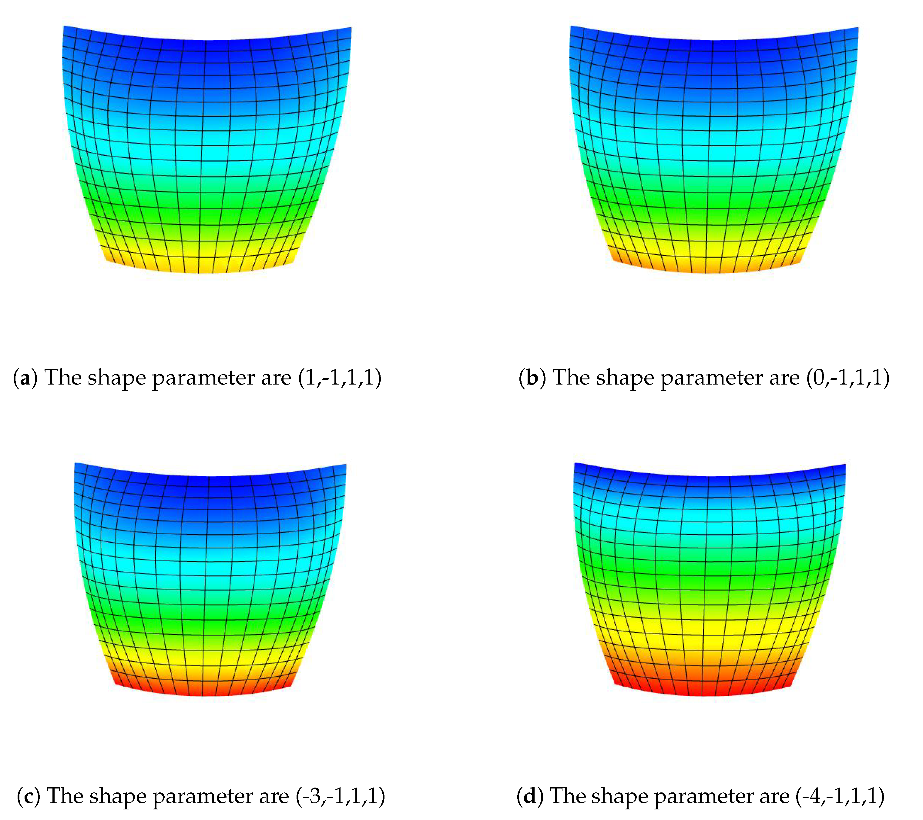
Figure 11 shows the effect of shape parameter on shape adjusting surfaces with mean curvature when the four boundary curves are fixed (interpolated with traditional Bézier curves), while the inside of surface shape is changed according to the changes in shape parameter values. Figure 11a–d, the value of shape parameters ${\alpha }_v$ and ${\beta }_v$ are equal to one, but value of ${\alpha }_u$ is changing in the range of $[-4,1]$ and ${\beta }_u$ has a value of $-1$. Similarly, we can get more results by altering the values of ${\beta }_u$ and also by changing parameter values ${\alpha }_v$ and ${\beta }_v$ by fixing the parameter values in the u-direction.

9. Conclusions

In this paper, we present the shape adjustable surfaces using quintic trigonometric Bézier basis function and study the effect of adjustable shape parameters on the shape of surfaces. The work contains the following two aspects. Firstly, we discuss the theory of constructing the generalized Bézier surface, swept surface and swung surface using a quintic trigonometric Bézier curve with four shape parameters. Then $G^2$ continuity conditions for the biquintic trigonometric Bézier surfaces are derived and the impact rules of the shape parameters on the splicing surface are assessed. Furthermore, examples are given to visually analyze the effect of shape parameters on different types of surfaces. Secondly, we adopted the mean curvature nephogram to show the effect of the shape parameter at the inside of the surface. In addition to this, we construct the Coons surfaces that have the characteristic of both the traditional Bézier curve and quintic trigonometric Bézier curve and show the effect of altering the shape parameter values with fixed boundary curves. This type of surface has a great significance in advance modeling such as in the automobile industry.

Cubic trigonometric polynomial and NURBS usually can construct surfaces with some restrictions and limitations due to the control point need to be alter to get desired shape. In this paper, quintic trigonometric Bézier curve with shape parameters demonstrated smooth surface by possessing the similar properties as cubic trigonometric polynomial and NURBS. The position of control points can be fixed by using this method and at the same time the shape of the surface can be varied.

However, future work is suggested to be done involving the construction of more complex surfaces by inheriting all the geometric properties of the traditional Bézier curve with smooth joining of the quintic trigonometric Bézier curves.

References

1. Bashir, U.; Abas, M.; Awang, M.; Ali, J. The quadratic trigonometric Bézier curve with single shape parameter. J. Basic Appl. Sci. Res. 2012, 2, 2541–2546. [Google Scholar]
2. Bashir, U.; Abbas, M.; Majid, A.A.; Ali, J.M. The Rational Quadratic Trigonometric Bézier Curve with Two Shape Parameters. In Proceedings of the 2012 Ninth International Conference on Computer Graphics, Imaging and Visualization, Hsinchu, Taiwan, 25–27 July 2012; pp. 31–36. [Google Scholar]
3. Wu, X.; Han, X. Cubic trigonometric polynomial curves with a shape parameter. Comput. Appl. Softw. 2007, 24, 62–64. [Google Scholar]
4. Yan, L. Cubic trigonometric nonuniform spline curves and surfaces. Math. Probl. Eng. 2016, 2016, 7067408. [Google Scholar] [CrossRef] [Green Version]
5. Han, X.; Ma, Y.; Huang, X. The cubic trigonometric Bézier curve with two shape parameters. Appl. Math. Lett. 2009, 22, 226–231. [Google Scholar] [CrossRef] [Green Version]
6. Misro, M.Y.; Ramli, A.; Ali, J.M.; Hamid, N.N.A. Cubic trigonometric Bézier spiral curves. In Proceedings of the 2017 14th International Conference on Computer Graphics, Imaging and Visualization, Marrakesh, Morocco, 23–25 May 2017; pp. 14–20. [Google Scholar]
7. Misro, M.Y.; Ramli, A.; Ali, J.M. Extended analysis of dynamic parameters on cubic trigonometric Bézier transition curves. In Proceedings of the 2019 23rd International Conference in Information Visualization—Part II, Adelaide, Australia, 16–19 July 2019; pp. 141–146. [Google Scholar]
8. Dube, M.; Sharma, R. Quartic trignometric Bézier curve with a shape parameter. Int. J. Math. Comput. Appl. Res. 2013, 3, 89–96. [Google Scholar]
9. Han, X. Piecewise quartic polynomial curves with a local shape parameter. J. Comput. Appl. Math. 2006, 195, 34–45. [Google Scholar] [CrossRef] [Green Version]
10. Misro, M.; Ramli, A.; Ali, J. Quintic trigonometric Bézier curve with two shape parameters. Sains Malays. 2017, 46, 825–831. [Google Scholar]
11. Misro, M.Y.; Ramli, A.; Ali, J.M.; Hamid, N.N.A. Pythagorean hodograph quintic trigonometric Bézier transtion curve. In Proceedings of the 2017 14th International Conference on Computer Graphics, Imaging and Visualization, Marrakesh, Morocco, 23–25 May 2017; pp. 1–7. [Google Scholar]
12. Yan, L.; Liang, J. A class of algebraic–trigonometric blended splines. J. Comput. Appl. Math. 2011, 235, 1713–1729. [Google Scholar] [CrossRef]
13. Li, J. A Class of Cubic Trigonometric Automatic Interpolation Curves and Surfaces with Parameters. Math. Comput. Appl. 2016, 21, 18. [Google Scholar] [CrossRef] [Green Version]
14. Cao, J.; Wang, G.Z. Non-uniform B-spline curveswith multiple shape parameters. J. Zhejiang Univ. Sci. C 2011, 12, 800. [Google Scholar] [CrossRef]
15. Misro, M.; Ramli, A.; Ali, J. S-shaped and c-shaped transition curve using cubic trigonometric Bézier. In AIP Conference Proceedings; AIP Publishing LLC Melville: New York, NY, USA, 2017; Volume 1870, p. 050005. [Google Scholar]
16. Yang, L.; Zeng, X.M. Bézier curves and surfaces with shape parameters. Int. J. Comput. Math. 2009, 86, 1253–1263. [Google Scholar] [CrossRef]
17. Wu, H. Extensions of Bézier Curves and Surfaces with Multiple Shape Parameters. J. Comput. Aided Des. Comput. Graph. 2005, 12, 2607. [Google Scholar]
18. Su, B.Y.; Tan, J.Q. A family of quasi-cubic blended splines and applications. J. Zhejiang Univ.-Sci. A 2006, 7, 1550–1560. [Google Scholar] [CrossRef]
19. Chand, A.; Tyada, K. Partially blended constrained rational cubic trigonometric fractal interpolation surfaces. Fractals 2016, 24, 1650027. [Google Scholar] [CrossRef]
20. Liu, X.; Xu, W. Uniform B-Spline Curve and Surface with Shape Parameters. In Proceedings of the 2008 International Conference on Computer Science and Software Engineering, Wuhan, China, 22 December 2008; Volume 2, pp. 975–979. [Google Scholar]
21. Hu, G.; Cao, H.; Wang, X.; Qin, X. G2 continuity conditions for generalized Bézier-like surfaces with multiple shape parameters. J. Inequal. Appl. 2017, 2017, 248. [Google Scholar] [CrossRef] [PubMed] [Green Version]
22. Lasser, D. Tensor product Bézier surfaces on triangle Bézier surfaces. Comput. Aided Geom. Des. 2002, 19, 625–643. [Google Scholar] [CrossRef]
23. Hu, G.; Ji, X.M.; Shen, X.Q.; Song, W.J. Research on the continuity conditions for CE-Bézier surfaces. J. Graph. 2012, 33, 62–67. [Google Scholar]
24. Farin, G.E.; Farin, G. Curves and Surfaces for CAGD: A Practical Guide; Morgan Kaufmann: San Fransisco, CA, USA, 2002. [Google Scholar]
25. Piegl, L.; Tiller, W. The NURBS Book; Springer Science & Business Media: New York, NY, USA, 2012. [Google Scholar]
Figure 1. Quintic trigonometric Bézier basis function.
Symmetry 12 01205 g001
Figure 2. Biquintic trigonometric Bézier surface with different shape parameter values.
Symmetry 12 01205 g002aSymmetry 12 01205 g002b
Figure 3. G2 continuity condition in the u-direction between two adjacent biquintic trigonometric Bézier surfaces at different scale factor and shape parameter values.
Symmetry 12 01205 g003
Figure 4. Defining a swept surface using a section curve and trajectory curve.
Symmetry 12 01205 g004
Figure 5. Translational swept surface with different shape parameter values.
Symmetry 12 01205 g005aSymmetry 12 01205 g005b
Figure 6. Defining a swung surface using profile and trajectory curves.
Symmetry 12 01205 g006
Figure 7. Swung surface with different scaling factors.
Symmetry 12 01205 g007aSymmetry 12 01205 g007b
Figure 8. Swung surface with different shape parameter values.
Symmetry 12 01205 g008aSymmetry 12 01205 g008b
Figure 9. Effect of shape parameters α u , β u and α v , β v in surface designing shown with mean curvature without fixing boundary curves.
Symmetry 12 01205 g009
Figure 10. (a) The surface R 1 ( u , v ) defined in Equation (44) with traditional Bézier basis function in the u-direction (blue color) and quintic trigonometric Bézier basis function in the v-direction (red color). (b) The surface R 2 ( u , v ) defined in Equation (45) with traditional Bézier basis function in the v-direction and quintic trigonometric Bézier basis function in the u-direction. (c) The Coon surface T ( u , v ) defined in Equation (46), constructed by four quintic trigonometric Bézier curves. (d) The final biquintic-Coons surface S ( u , v ) .
Symmetry 12 01205 g010
Figure 11. Effect of shape parameters α u , β u in surface design shown with mean curvature with fixed boundary curves.
Symmetry 12 01205 g011