Optimizing Minimum Headway Time and Its Corresponding Train Timetable for a Line on a Sparse Railway Network

Abstract

In western China, railway lines are sparse, and there is a large fluctuation in transport demand under different transportation scenarios, which yields severe difficulties in setting up a signaling system and making a train timetable. To meet the fluctuating transport demand effectively and provide efficient train services in the changing multimodal transportation market, a new Chinese train control system based on flexible minimum headway time (FCTCS) is introduced and going to be implemented. Considering that the cost of implementing signaling systems corresponding to different minimum headway times varies significantly, it is necessary to find an optimal minimum headway time and design its corresponding train timetable. In this paper, we propose a mixed integer linear programming model for selecting an optimal minimum headway time, with which a satisfactory train timetable is generated with the consideration of symmetry transport demand. The objective function is to maximize the total profit of train operation. We further develop genetic algorithm with an integer and binary coding method for searching for the solution. Finally, a set of numerical tests based on a railway line in a sparse railway network in western China is used to demonstrate the validity and effectiveness of the proposed model.

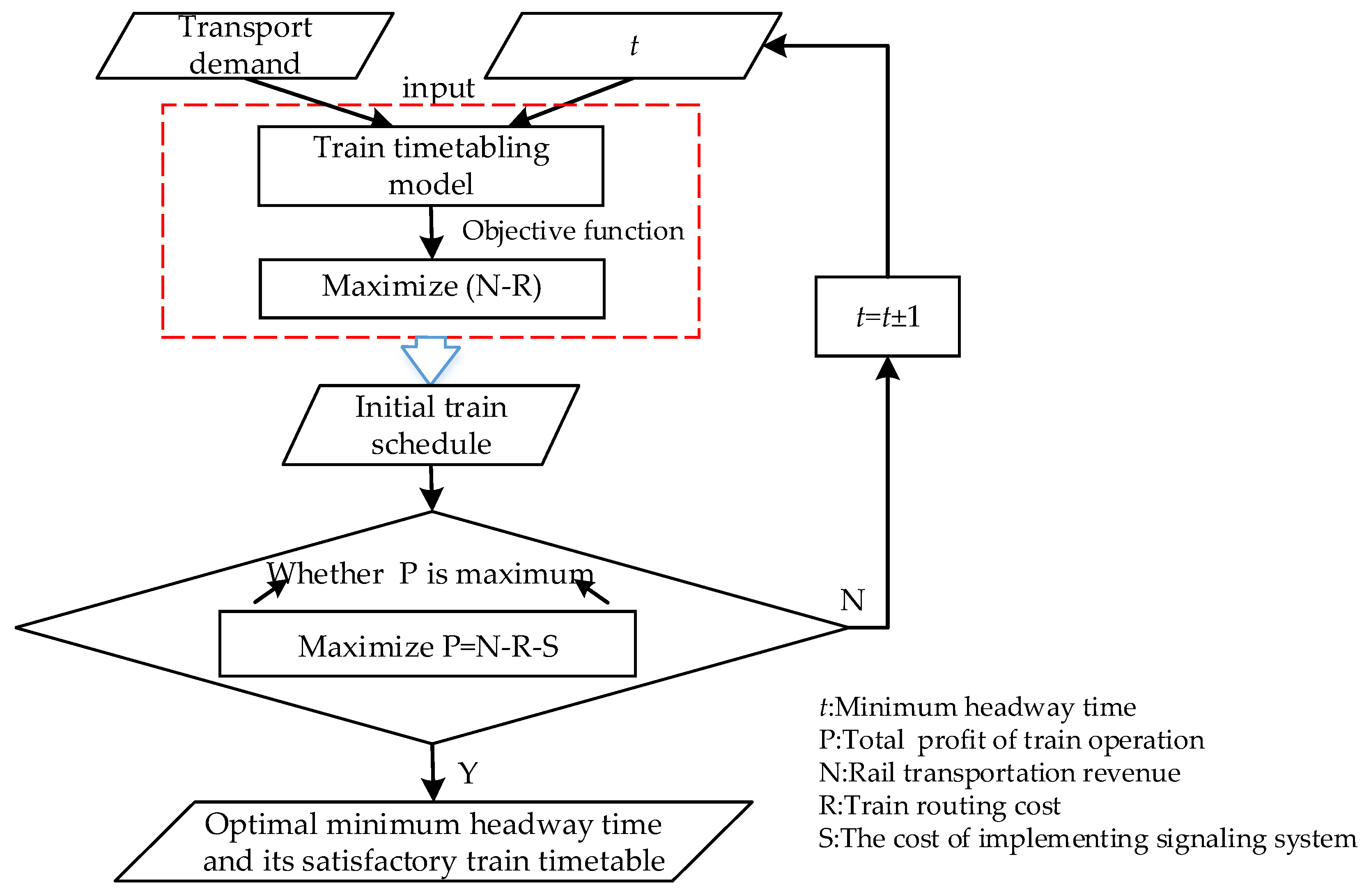
1. Introduction

Compared with the complex railway network in eastern China, the railway lines in western China are sparse. In a normal transportation scenario, the transport demand in western area is generally low; however, during some special periods, the transport demand increases sharply, which brings a great challenge for train operation on these sparse lines. When higher demand occurs, the provided signaling resource may not adequately meet the given demand. Although we can operate trains with a longer headway—compared with the minimum one based on the existing signaling system, where the minimum headway time remains the same—it will also lead to a waste of signaling resources as implementing excessive signaling resources generates costs, especially in such areas with fluctuating demand and not so good operational conditions. Therefore, a new Chinese train control system based on flexible minimum headway time (FCTCS) is introduced and going to be implemented to attempt to meet the fluctuating transport demand for sparse railway lines. Using the new signaling system, it is more flexible to operate trains corresponding to the generated demand and makes it possible to save more operational costs, due to the flexible minimum headway. To explain clearly about the flexible minimum headway in FCTCS, we illustrate it in Figure 1.

Based on the new proposed FCTCS, train timetabling is therefore required to optimize. In view of the characteristic of flexible minimum headway in FCTCS, we consider the corresponding cost of implementing signaling systems in train timetabling, and make efforts to maximize the profit of train operation. In addition, transport demand is regarded as an essential element in solving a train timetabling problem. Generally, after a demand analysis, the train timetable is constructed to determine the departure and arrival time of each train at each station, which is a sequential process. However, in many real-world cases, the transport demand fluctuates randomly, and the obtained train schedule in the latter step might not satisfy the demand in such a sequential process. As a result, embedding transport demand into the train timetable phase has gradually attracted more attention.

In this paper, based on flexible minimum headway in FCTCS, we focus on finding an optimal minimum headway time with which a satisfactory train timetable is designed to well satisfy the fluctuating transport demand. Although the problem of optimizing train timetables was often investigated, the optimization of minimum headway time to make the train timetable design more adaptive to the fluctuating transport demand was paid less attention, and can still be improved. Here, we give a method of how to select the optimal minimum headway in train timetabling, which can be used to support the planning decisions. Furthermore, innovated by the flexibility of minimum headway time, the train timetable can still be well-designed with the cost of implementing signaling system corresponding to different minimum headways considered in the objective function, because, for train operators, the greatest concern is how to maximize the profit of train operation after satisfying demand. The cost of implementing signaling system has a great impact on train operational costs. Thus, a methodology is proposed to select an optimal minimum headway with the cost of implementing signaling system corresponding to different minimum headways and is considered in this study to fill in the gap of optimizing minimizing headway time in train timetabling.

To solve this problem, a mixed integer linear programming model is formulated, in which the transport demand corresponding to different origin and destination stations, train stop planning, train routing and train timetabling are included in the model formulation. In this train timetabling process, first of all, the transport demand and minimum headway time are regarded as inputs into the proposed train timetabling model, to obtain an initial train schedule with an objective function of maximizing the profit of rail transportation revenue and train routing cost. Then, we vary the minimum headway time t to evaluate the initial train timetable by maximizing the total operational profit of rail transportation revenue, train routing cost and the cost of implementing signaling system. Finally, we obtain the optimal minimum headway time and its corresponding train timetable. The whole optimization process in this paper is shown in Figure 2.

The remainder of this paper is organized as follows. Section 2 provides a literature review on three areas: train timetabling, train timetabling considering transport demand, as well as optimizing headway for train timetable. In Section 3, conditions of the model are given, followed by a mathematical model that formulates the optimization problem. Next, a genetic algorithm is introduced to solve the proposed model in Section 4. In Section 5, the proposed model and algorithm are applied on a railway line of a sparse railway network in western China to evaluate their validity. Finally, conclusions and future research are presented in Section 6.

2. Literature Review

In this section, we review the state-of-the-art in three parts: (1) train timetabling; (2) train timetabling considering transport demand; (3) optimizing headway for train timetable.

Train timetabling plays an important role in train operations and several researchers have investigated this problem with a variety of models and algorithms [1,2,3,4,5,6]. Based on the job-shop scheduling problem, Szpigel (1973) first modeled the single-track train scheduling problem to determine the location of crossing and overtaking [7]. Carey and Lockwood (1995) designed a mathematical model and algorithm for the train pathing and timetabling problem on a double-track railway line [8]. Higgins, Kozan and Ferreira (1996) scheduled trains optimally on a single-line track and presented a lower bound to reduce the search space in the branch and bound tree [9]. Caprara et al. (2002,2006) provided a graph description of the train timetabling problem with a fixed train running time and headway time [10,11]; however, this approach is not practical due to train acceleration and deceleration. Ghoseiri et al. (2004) used a multi-objective model to balance the satisfaction of railway companies and passengers, which was solved by the Pareto frontier [12]. Zhou and Zhong (2007) used branch-and-bound solution algorithms to solve a single-track train timetabling problem, and generalized station headway capacities-constrained scheduling formulation [13]. Based on the time-space network, Lusby et al. (2011) represented train timetabling by illustrating the occupation of time-space resources and used multiple heuristic algorithms to solve the problem [14]. Mu and Dessouky (2011) developed two optimization algorithms to solve the freight train scheduling problem on an N-track network in the US [15]. Yang et al. (2016) considered the uncertain dwell time and formulated the timetable optimization problem as a bi-objective expected value model [16].

We now move to a brief review on train timetabling considering transport demand. In recent years, studies on demand-sensitive train timetabling have attracted increasing attention, with the goal of providing a high level of train service to satisfy demand. Sun et al. (2014) provided a demand-driven timetable for metro services, which adjusted service frequency dynamically instead of fixing it for peak/off-peak times respectively, aiming to minimize total passenger waiting time [17]. Barrena et al. (2014) proposed three exact linear formulations and the branch-and-cut algorithm to design train timetables that were consistent with dynamic demand [18]. To solve large-scale instances, Barrena et al. (2014) presented an adaptive large neighborhood search (ALNS) meta-heuristic model [19]. Canca et al. (2014) and Cheng and Peng (2014) considered elastic passenger demand and optimized the train timetable. Based on time-varying origin–destination demand [20,21]. Niu, Zhou and Gao (2015) proposed quadratic and quasi-quadratic objective functions to formulate total passenger waiting time [22]. Wang et al. (2015,2018) then concentrated on the time-varying passenger demand of the segment between two adjacent stations to integrate train scheduling and rolling stock circulation planning for an urban rail transit line [23,24]. Furthermore, Robenek et al. (2018) studied the unknown demand elasticities with using a logit model [25]. These aforementioned studies on timetable optimization usually featured models based on the pre-planned stop pattern, which cannot optimize the stop pattern at the same time. Therefore, some studies furthered train stop plan optimization in timetabling [26,27,28]. Qi, Cacchiani and Yang (2018) emphasized uncertain passenger demand and aimed to determine both train timetables and stop plans [29].

Headway time is a vital factor to detect train conflicts in the process of train timetabling. Given that transport demand has large variations, train timetables with fixed headways cannot satisfy fluctuating demand well [30]. Furthermore, most optimization models that deal with train timetables treat the minimum headway required between consecutive trains as given constants. However, this is not very practical. As a consequence, improved studies that take flexible headways into consideration have been proposed [31,32,33,34]. Lee and Chen (2009) let the minimum headway between the trains depend on the trains’ relative status (track assignment), instead of regarding it as a constant [35]. Khoshniyat and Peterson (2017) proposed an idea of travel time dependent scheduled minimum headway, which was to reserve a triangular time slot for trains’ arrival times, instead of a fixed-sized time slot [36]. In terms of optimizing the minimum headway time, Sangphong, Siridhara and Ratanavaraha (2017) determined the minimum train headway by train speed and the maximum block length in a fixed-block system to maximize rail line capacity, which was applied to both equal and unequal block length situations [37]. Liu and Han (2017) also distinguished different headway time in train timetabling and tried to obtain a feasible timetable with more scheduled trains [38]. Zhang and Han (2011) constructed a train headway optimization programming model to optimally use the minimum train headway with an objective function of maximizing reliability [39]. Apart from the mostly used integer programming in the aforementioned research, simulation methods were also adopted to optimize the minimum headway time. Based on active communications, Zhao and Ioannou (2015) adopted a simulation model to calculate dynamic minimum headway in a headway selection loop, and then used it to solve a train dispatching problem [40].

Regarding the past studies, we can see that a lot of studies considered fluctuating transport demand and optimized headways in train timetabling. Many researchers concentrated on scheduling trains to satisfy the demand, but few of them optimized the timetable from the viewpoint of selecting the optimal minimum headway to design a satisfactory train timetable with the given demand. In this work, we focus on finding an optimal minimum headway in train timetabling, with which a satisfactory train timetable can be designed to be adaptive to the fluctuating transport demand. Furthermore, in the process of optimizing headways, most studies optimized the scheduled headway between consecutive running trains, instead of the technical minimum headway that we study in this work. Finally, few studies on train timetabling were found with the consideration of the cost of implementing signaling systems. This should not be ignored, because the flexibility in minimum headway has an important influence on the variation in the cost of implementing signaling system corresponding to different minimum headways. In this paper, the corresponding cost is included into the objective function to maximize the train operational profit.

Therefore, this paper makes the following two contributions.

• In view of the flexible minimum headway time in FCTCS, this work tries to find the optimal minimum headway time by varying the minimum headway in a set of given minimum headways and generates a satisfactory train timetable. A linear programming model is built, rigorously considering the cost of implementing signaling systems corresponding to different minimum headway time, which makes it possible to save signaling resources, as well as to well satisfy the fluctuating transport demand.
• In the proposed model, we also embed transport demand into the train timetabling stage and simultaneously optimize the train timetable, as well as the stop plan, which satisfies the demand more flexibly.

3. Mathematical Model

3.1. Conditons of the Model

Before the mixed-integer linear programming model is described, inputs, key decision variables and model assumptions are given sequentially. First, inputs of this problem are explained as follows:

1. A railway network based on a railway line

A railway network is given with a number of stations and segments between consecutive stations, which are represented by physical nodes and physical cells. Each segment and each station on a rail line are set as one cell, respectively.

2. A set of trains

For each train, we know its origin and destination station, the earliest starting time at its origin station, the running time between two consecutive stations, the minimum and maximum dwell time at intermediate stations, a set of minimum headway time, the train carrying capacity and the train characteristics.

3. Transport demand pairs

In this paper, we consider transport demand as a number of demand pairs with different origin and destination stations. For each demand pair, we know its origin station, destination station and demand pair volume.

The train timetabling problem based on FCTCS has the following key decision variables

• For each planned train, we need to determine its departure time at the origin station, the arrival, dwell time, and departure time at intermediate stations, and the arrival time at the destination station. In addition, we also need to determine its stop plan, i.e., whether the train chooses to stop and how long it will stop at a station.
• For each demand pair, we need to determine which train delivers the demand pair and how many of the transport demand is delivered in the demand pair.

In our model, we assume that:

• The responses of demand to the resulting train service, such as travelers’ choices, are not considered in this work. As dynamic choice behaviors of travelers can influence the underlying train service patterns and detailed timetables, such as service interval times or frequencies, we assume that the transport demand is assigned to take trains in equal proportions.
• For simplicity, we simplify the detailed calculation of $\phi \left(t\right)$ into a simple decreasing function in this work and directly give corresponding costs with the variation in t. The relation between minimum headway time t and the implementing signaling system cost function $\phi \left(t\right)$ is complex. Moreover, it is obvious to see that the cost decreases with t increasing, because the increasing t can save more signaling resources.
• The price is roughly estimated based on the distance. Although our objective is to maximize train operational profit, we concentrate on selecting an optimal minimum headway in a train timetabling model instead of making price decisions.
• The minimum dwell time is fixed without changing with demand fluctuations at a station. If the minimum dwell time is regarded as a variable influenced by the fluctuating demand, it is difficult to evaluate the influence of varying minimum headway on train timetable.
• The station can accommodate enough trains, which means that the station capacity is not constrained. Our model is at a macroscopic level, regardless of detailed track assignment in a station.
• It should be noted that the granularity of minimum headway time is one minute in this work, or a shorter time interval (if required).

The general subscripts and input parameters of the proposed formulations are introduced in

Table 1. General subscripts.

Symbol	Description
$i,j,k$	Physical node index, $i,j,k\in N$, N is the set of nodes.
$e$	Physical cell index, $e\in E$, E is the set of cells.
$p$	Transport demand origin-destination (OD) pair index, $p,p\prime \in P$, P is the set of transport demand OD pairs. One demand OD pair refers to a group of transport demands who have the same origin and destination stations.
$f$	Train index, $f\in F$, F is the set of trains that need to be scheduled.
$t,t\prime$	Minimum headway time, $t,t\prime \in I$, $t\prime =t\pm 1$, I is the set of given minimum headway time.
$m,m\prime$	Station index, $m,m\prime \in S$, S is the set of all stations.

and

Table 2. Input parameters.

Symbol	Description
$E_f^{}$	Set of cells train f may use, $E_f^{}\subset E$.
$E_s^{}$	Set of station cells, $E_s^{}\subset E$.
$E_c^{}$	Set of segment cells, $E_c^{}\subset E$.
$E_i^{\mathrm{o}}$	Set of cells starting from node i.
$E_i^{\mathrm{s}}$	Set of cells ending at node i.
${\delta }_{f,i,j}$	Free-flow running time for train f to drive through cell (i, j).
${\vartheta }_{f,i,j}^{\min }$	Minimum dwell (waiting) time for train f on cell (i, j).
${\vartheta }_{f,i,j}^{\max }$	Maximum dwell (waiting) time for train f on cell (i, j).
$T{T}_{f,i,j}$	Travel time for train f on cell (i, j).
$O_f$	Origin node of train f.
$S_f$	Destination (sink) node of train f.
$O_m$	Origin node of station m.
$S_m$	Destination (sink) node of station m.
$m_p^o$	Origin station of demand pair p.
$m_p^s$	Destination station of demand pair p.
$ES{T}_f$	Predetermined earliest starting time of train f at its origin node.
${\eta }_p$	Volume of demand OD pair p.
$C_f$	The capacity of train f.
$\alpha$	The maximum demand carrying coefficient of the scheduled trains.
$\phi (t)$	The implementing signalling system cost function when minimum headway time is t.
$C{T}_{f,i,j}$	The cost when train f traverses on cell (i, j).
$R_{f,p}$	The rail transportation revenue when train f carries transport demand pair p.
$k_{p,i,j}$	0–1 binary demand pair p routing variables, =1, if demand pair p travel on cell (i, j), =0 otherwise.
M	A sufficiently large positive number.

respectively, and the decision variables are provided in

Table 3. Input parameters.

Symbol	Description
$a_{f,i,j}$	The arrival time of train f at cell (i, j).
$d_{f,i,j}$	The departure time of train f at cell (i, j).
$x_{f,i,j}$	0–1 binary train routing variables, =1, if train f selects cell (i, j) on the network; =0 otherwise.
${\theta }_{f,f\prime ,i,j}$	0–1 binary train ordering variables, =1, if train f’ arrives at cell (i, j) after train f; =0 otherwise.
$y_{f,p}$	Transport demand variables, transport demand of demand pair p that is transported by train f.
$z_{f,p,i,j}$	Transport demand variables on cell (i, j), transport demand of demand pair p that is transported by train f on cell (i, j).
$r_f^{m,m\prime }$	0–1 binary train stopping variables, =1, if train f stops at both station m and m’, =0 otherwise.

.

3.2. Formulation of the Model

As we have explained in Section 1, the objective function in our train timetabling work considers two parts. First of all, we consider train routing costs and maximize the difference between rail transportation revenue and train routing costs, in order to obtain an initial train timetable. Then, based on the initial timetable, we consider the different given costs of implementing signaling systems with flexible minimum headway $\phi \left(t\right)$ and maximize the total profit of train operation, in order to obtain an optimal minimum headway time from a set as well as its corresponding train timetable.

Therefore, the objective function can be presented as follows.

$$\max Z={\displaystyle \sum _{p\in P}{\displaystyle \sum _{f\in F}{y}_{f,p}}}\times R_{f,p}-{\displaystyle \sum _{f\in F}{\displaystyle \sum _{i,j:(i,j)\in E_f}C{T}_{f,i,j}}}\times x_{f,i,j}-\phi \left(t\right)$$

(1)

For clarity, the constraints of the optimization problem can be divided into several groups, namely train timetabling constraints, transport demand constraints, and mapping constraints between transport demand and stopping pattern, which are shown sequentially as below.

Group 1: Train timetabling constraints

In a train timetabling problem, all trains are supposed to meet the flow balance when the train runs on the railway network. In this model, we divide the nodes in the network into three types of nodes (origin node, intermediate node and destination node) to explain the flow balance problem. At the origin node and destination node, there is only one routing choice for train f to go through. Constraints (2)–(4) ensure flow balance on the railway network at the origin node, the intermediate nodes and the destination node of train f, respectively.

$${\displaystyle \sum _{i,j:(i,j)\in E_{o_f}^{\mathrm{o}}\cap E_f}{x}_{f,i,j}}=1,\forall f\in F$$

(2)

$${\displaystyle \sum _{i:(i,j)\in E_j^{\mathrm{s}}\cap E_f}{x}_{f,i,j}}={\displaystyle \sum _{k:(j,k)\in E_j^{\mathrm{o}}\cap E_f}{x}_{f,j,k}},\forall f\in F,j\in N\backslash \left\{o_f,s_f\right\}$$

(3)

$${\displaystyle \sum _{i,j:(i,j)\in E_{s_f}^{\mathrm{s}}\cap E_f}{x}_{f,i,j}}=1,\forall f\in F$$

(4)

Train timetabling is actually to determine train routes on a time-space network. Hence, constraints (5)–(8) are time-space network constraints for train f.

In the time-space network, a train’s starting time is required to ensure that the train departs within a given time. For a train’s starting time, constraints (5) ensure that each train does not depart earlier than its predetermined earliest starting time at its origin station. Within the cell-to-cell transition, constraints (6) enforce the departure time on cell (i, j) and the arrival time of adjacent cell (j, k), when they are both used by train f.

$${\displaystyle \sum _{j:(o_f,j)\in E_f}{a}_{f,o_f,j}}+\left(1-x_{f,i,j}\right)\times M\ge ES{T}_f, \forall f\in F$$

(5)

$${\displaystyle \sum _{i,j:\left(i,j\right)\in E_f}{d}_{f,i,j}}={\displaystyle \sum _{j,k:\left(j,k\right)\in E_f}{a}_{f,j,k}}, \forall f\in F,j\in N\backslash \left\{o_f,s_f\right\}$$

(6)

Constraints (7) and (8) are mapping constraints between time-space network and physical network.

$$x_{f,i,j}-1\le a_{f,i,j}\le x_{f,i,j}\times M, \forall f\in F,\left(i,j\right)\in E_f$$

(7)

$$x_{f,i,j}-1\le d_{f,i,j}\le x_{f,i,j}\times M, \forall f\in F,\left(i,j\right)\in E_f$$

(8)

Here, we use the decision variables $a_{f,i,j}$ and $d_{f,i,j}$ to represent the running time $T{T}_{f,i,j}$, the value of which is the difference between the exit time and entrance time for train f on cell (i, j), shown by constraints (9).

$$T{T}_{f,i,j}=d_{f,i,j}-a_{f,i,j},\forall f\in F,(i,j)\in E_f$$

(9)

In real-world cases, due to train stops and some unexpected disturbances, the total running time on cell (i, j) must be equal or larger than its free-flow travel time. Constraints (10) specify this scenario in an inequality. Then, constraints (11) enforce the maximum planned dwell time at a station.

$${\delta }_{f,i,j}\le T{T}_{f,i,j}+\left(1-x_{f,i,j}\right)\times M,\forall f\in F,(i,j)\in E_f$$

(10)

$${\vartheta }_{f,i,j}^{\max }+{\delta }_{f,i,j}\ge T{T}_{f,i,j}+\left(x_{f,i,j}-1\right)\times M,\forall f\in F,(i,j)\in E_f\cap E_s$$

(11)

Constraints (12)–(14) link train order variables and train routing variables. Specifically, constraints (13) make sure that only if both train f and f’ traverse on cell (i, j) ($x_{f,i,j}=x_{f\prime ,i,j}=1$), then ${\theta }_{f,f\prime ,i,j}+{\theta }_{f\prime ,f,i,j}$ is constrained to be the value of 1, which means that either train f arrives after train f’ at cell (i, j) or train f’ arrives after train f at cell (i, j). If $x_{f,i,j}=1$, $x_{f\prime ,i,j}=0$ or $x_{f,i,j}=0$, $x_{f\prime ,i,j}=1$, or $x_{f,i,j}=0$, $x_{f\prime ,i,j}=0$, then the inequality of constrains (12) reduce to be non-active as the value of ${\theta }_{f,f\prime ,i,j}+{\theta }_{f\prime ,f,i,j}$ returns between 0 to 2. In addition, constraints (13) and (14) ensure that any ${\theta }_{f,f\prime ,i,j}$ and ${\theta }_{f\prime ,f,i,j}$ are always less than $x_{f,i,j}$ and $x_{f\prime ,i,j}$.

$$x_{f,i,j}+x_{f\prime ,i,j}-1\le {\theta }_{f,f\prime ,i,j}+{\theta }_{f\prime ,f,i,j}\le 3-x_{f,i,j}-x_{f\prime ,i,j},\forall f,f\prime \in F,f\ne f\prime ,(i,j)\in E_f\cap E_{f\prime }$$

(12)

$${\theta }_{f,f\prime ,i,j}\le x_{f,i,j},\forall f,f\prime \in F,f\ne f\prime ,(i,j)\in E_f\cap E_{f\prime }$$

(13)

$${\theta }_{f,f\prime ,i,j}\le x_{f\prime ,i,j},\forall f,f\prime \in F,f\ne f\prime ,(i,j)\in E_f\cap E_{f\prime }$$

(14)

Constraints (15)–(16) ensure the cell capacity requirement by using a given minimum safety headway time t if both two trains are running on the same segment cell (i, j). They make sure that only if both train f and f’ traverse the same cell, the time interval between the arrival times of a preceding train and a following train should respect the headway time t. Otherwise, when either train f or f’ does not traverse cell (i, j), constraints (15) and (16) reduce to be non-active. Then, we vary t in these two constraints to optimize train timetable based on FCTCS.

$$\begin{array}{l}{a}_{f\prime ,i,j}+(3-x_{f,i,j}-x_{f\prime ,i,j}-{\theta }_{f,f\prime ,i,j})\times M\ge a_{f,i,j}+t,\\ \forall f,f\prime \in F,f\ne f\prime ,(i,j)\in E_f\cap E_{f\prime }\cap E_c,t\in I\end{array}$$

(15)

$$\begin{array}{l}{a}_{f,i,j}+(3-x_{f,i,j}-x_{f\prime ,i,j}-{\theta }_{f\prime ,f,i,j})\times M\ge a_{f\prime ,i,j}+t,\\ \forall f,f\prime \in F,f\ne f\prime ,(i,j)\in E_f\cap E_{f\prime }\cap E_c,t\in I\end{array}$$

(16)

Group 2: Transport demand constraints

Constraints (17) ensure that for each demand pair, the total amount of the transport demand carried by all planned trains is supposed to be no more than the volume of the demand pair. In addition, constraints (18) indicate that for each train scheduled, the total amount of the transport demand of all demand pairs that can be assigned to a train is limited by its maximum carrying capacity. Constraints (19) are mapping constraints between $z_{f,p,i,j}$ and $y_{f,p}$ by using a binary demand routing variable $k_{p,i,j}$.

$${\displaystyle \sum _{f:f\in F}{y}_{f,p}}\le {\eta }_p,\forall p\in P$$

(17)

$${\displaystyle \sum _{p:p\in P}{z}_{f,p,i,j}}\le \alpha \times C_f,\forall f\in F,\left(i,j\right)\in E_f$$

(18)

$$z_{f,p,i,j}=y_{f,p}\times k_{p,i,j},\forall f\in F,p\in P,\left(i,j\right)\in E_f$$

(19)

Group 3: Mapping constraints between transport demand and stopping pattern

The following constraints present that if train f carries demand pair p, then the train needs to stop at both the origin station and the destination station of demand pair p to deliver demand pair p. Constraints (20) explain this scenario in an inequality.

$$y_{f,p}\le r_f^{m_p^o,m_p^s}\times M,\forall f\in F,p\in P$$

(20)

Further, if train f stops at the origin station and destination station of demand pair p ($r_f^{m_p^o,m_p^s}=1$), it is supposed to provide enough dwell time at both stations for train f to pick up and drop off the transport demand. Therefore, constraints (21) and constraints (22) enforce the minimum waiting time for train f to dwell at the origin station and the destination station of demand pair p, respectively.

$$d_{f,i,S_{m_p^o}}-a_{f,O_{m_p^o},j}\ge {\vartheta }_{f,i,j}^{\min }+M\times (r_f^{m_p^o,m_p^s}-1),\forall f\in F,p\in P,\left(i,j\right)\in E_f$$

(21)

$$d_{f,i,S_{m_p^s}}-a_{f,O_{m_p^s},j}\ge {\vartheta }_{f,i,j}^{\min }+M\times (r_f^{m_p^o,m_p^s}-1),\forall f\in F,p\in P,\left(i,j\right)\in E_f$$

(22)

4. Genetic Algorithm for Solving the Train Timetabling Problem

The model proposed in this paper is a complex, mixed-integer programming problem, which enlarges the solution scale when the big-M method and train ordering variables are used in this model. In addition, considering transport demand in the train timetabling model further enforces the complexity and difficulty in solving the problem. It is difficult for commercial optimization solvers (i.e., Cplex) to solve such large-scale problem. Following a genetic algorithm (GA) that has been widely used to solve the train timetabling problem, GA is also adopted in this paper.

4.1. Representation of Chromosome and Generation of the Initial Population

The decision variables of the proposed model are shown as follows: transported demand pair volume, train routing, arrival and departure time and dwell time. Thus, the variables $y_{f,p}$, $x_{f,k}$, $d_{f,k}^m$ and $w_{f,k}^m$ collectively form the chromosome in the GA.

To code the chromosome in GA, the variables are divided into two parts. Transport demand assignment is the first part of the chromosome shown in Figure 3. Each train occupies p genes to transport the demand pairs as much as possible. Furthermore, variables of train routing, departure time at the first station and dwell time at the intermediate stations are the second part of the chromosome shown in Figure 4 to represent a train timetable. Each train has k routes available to traverse, but it can only choose one of them. $x_{f,k}$ is a binary variable that represents whether train f traverses on route k. $d_{f,k}^m$ represents the departure time at station m (m = 1,…, n, n is the number of traversed stations) when train f traverses on route k and $w_{f,k}^m$ represents the dwell time at station m. Both of these two parts compose an individual in GA shown in Figure 5.

Then, based on the coding approach, the following steps are performed to generate an initial population shown in Figure 6.

4.2. Calculation of the Fitness Function

As the objective function is to maximize the total train operation profit, a fitness function $f({\lambda }_q)$ is then defined in constraint (23) to determine the quality of each chromosome. Each chromosome is named as ${\lambda }_q$.

$$f({\lambda }_q)={\displaystyle \sum _{p\in P}{\displaystyle \sum _{f\in F}{y}_{f,p}}}\times R_{f,p}-{\displaystyle \sum _{f\in F}{\displaystyle \sum _{i,j:(i,j)\in E_f}C{T}_{f,i,j}}}\times x_{f,i,j}-\phi \left(t\right)$$

(23)

However, the initial population obtained in Section 4.1 might not be feasible. To obtain an unconstrained optimization problem, a penalty function is embedded in $f({\lambda }_q)$ to handle the constraints and update $f({\lambda }_q)$ to $f\prime ({\lambda }_q)$.

$$f\prime ({\lambda }_q)=\{\begin{array}{l}f({\lambda }_q),\mathrm{if}{\lambda }_q\mathrm{satisfies}\mathrm{the}\mathrm{constraints}.\\ f({\lambda }_q)-p({\lambda }_q),\mathrm{if}{\lambda }_q\mathrm{does}\mathrm{not}\mathrm{satisfy}\mathrm{the}\mathrm{constraints}.\end{array}$$

(24)

where $p({\lambda }_q)$ denotes the penalty function; $f({\lambda }_q)$ and $f\prime ({\lambda }_q)$ denote the initial fitness function and adjusted fitness function, respectively.

When the chromosome does not satisfy the constraints in the proposed model, the penalty function can be described by the following function.

$$p_i({\lambda }_q)=\{\begin{array}{l}0,\mathrm{if}{\lambda }_q\mathrm{satisfies}\mathrm{constraints}(i),i=1,\dots ,22.\\ M,\mathrm{if}{\lambda }_q\mathrm{does}\mathrm{not}\mathrm{satisfy}\mathrm{constraints}(i),i=1,\dots ,22.\end{array}$$

(25)

where M denotes a very large positive number.

Then, $f\prime ({\lambda }_q)$ can be reformulated into constraints (26).

$$f\prime ({\lambda }_q)={\displaystyle \sum _{p\in P}{\displaystyle \sum _{f\in F}{y}_{f,p}}}\times R_{f,p}-{\displaystyle \sum _{f\in F}{\displaystyle \sum _{i,j:(i,j)\in E_f}C{T}_{f,i,j}}}\times x_{f,i,j}-\phi \left(t\right)-{\displaystyle \sum _{i=1}^{22}{p}_i({\lambda }_q)}$$

(26)

4.3. Common Operators

Three common operators used in GA are selection, crossover and mutation.

1. Selection

The selection operator chooses the parents for the next generation based on their scaled values from the fitness function, which can provide a high objective value with an increased possibility to be selected and a low objective value with less possibility to be selected to conform the rule of survival of the fittest. The selection of chromosomes is done by spinning the roulette wheel. The selection probability of chromosome ${\lambda }_i$ is calculated by the following equation.

$$P_i=F_i/{\displaystyle \sum _{j=1}^n{F}_j}$$

(27)

where $F_i$ denotes the fitness value of chromosome ${\lambda }_i$ and n denotes the scale of the population. Then, the process of selection operation is shown as follows.

• Step 1. Set j = 1.
• Step 2. Randomly generate a number r$\in$ [0,1].
• Step 3. If $r\le q_1$, chromosome ${\lambda }_1$ is selected. If $q_{k-1}\le r\le q_k$ ($2\le k\le n$), chromosome ${\lambda }_k$ is selected. $q_i$ is the cumulative probability of chromosome ${\lambda }_i$ calculated by $q_i={\displaystyle \sum _{j=1}^i{P}_j}$.
• Step 4. If j$\ge$n, stop; otherwise, set j = j + 1 and go to Step 2.

2. Crossover

The crossover operation is used to combine two individuals or parents to form a new individual or child for the next generation. Assume that the probability of crossover operation is $P_c$. The process of crossover operation is shown as follows.

• Step 1. Randomly select two parents ${\lambda }_i$ and ${\lambda }_j$, and randomly generate a number r $\in$ [0,1].
• Step 2. If r$\le P_c$, then crossover operation will randomly select some positions of genes in two parts of the chromosome. In the first part of chromosome, randomly select multi-genes and perform crossover operation. While, in the second part, randomly select multi-genes representing train f and perform crossover operation.
• Step 3. Form two new individuals ${\lambda }_l$ and ${\lambda }_k$, shown in Figure 7.

3. Mutation

Moreover, the mutation operation produces small random changes in the individuals of the population; these changes provide genetic diversity and enable the GA to escape local optima. Assume that the probability of mutation operation is $P_m$. The process of mutation operation is shown as follows.

• Step 1. Randomly select one parent ${\lambda }_p$ and randomly generate a number r $\in$ [0,1].
• Step 2. If r$\le P_m$, then mutation operation will randomly select some genes from two parts of the chromosome and replace the genes with random numbers within the reasonable range. In the first part of chromosome, randomly select multi-genes and perform mutation operation. In the second part, randomly select multi-genes representing route k traversed by train f and perform mutation operation on $d_{f,k}^m$ and $w_{f,k}^m$.
• Step 3. Form a new chromosome ${\lambda }_q$, shown in Figure 8.

For every generation, the idea of elitism specifies the number of individuals that are guaranteed to survive to the next generation to ensure that the fast convergence of the GA is adopted.

4.4. Process of GA in Solving the Proposed Model

The process of the GA used to solve the proposed model is described in the following. The process contains the main operations (i.e., selection, crossover and mutation).

Step 1. Initialize.

Step 1.1. Initialize GA parameters: population, initial generation g = 1, and maximum number of generations G.

Step 1.2. Initialize model parameters: minimum/maximum dwell time at intermediate stations, earliest departure time at the first station, train capacity, the volume of each demand pair etc.

Step 1.3. Initialize a parent chromosome, including transported demand pair volume, train routing, train departure time at the first station and dwell time at the intermediate stations.

Step 1.4. Generate the chromosome until the number of chromosomes reaches the pop size.

Step 2. Create new population.

Step 2.1. Calculate the fitness function value with $f\prime ({\lambda }_q)$.

Step 2.2. Perform selection operation according to their fitness function values.

Step 2.3. Perform crossover operation.

Step 2.4. Perform mutation operation.

Step 2.5. Retain the elite children from the population after abovementioned operations and form a new population.

Step 3. Stop.

Step 3.1. Update g = g + 1.

Step 3.2. If g = G, then stop. Otherwise, return to Step 2.

End

5. Case Study

In this section, we implement several numerical experiments to show the validity and effectiveness of our proposed model, in which the Cplex solver is employed to code for a small-scaled example in Section 5.1 at first; then, the Matlab programming platform is used to produce a good solution with GA in Section 5.2 to solve a large-scaled case for a line on a sparse railway network. The following experiments are all performed on a server with two Intel(R) Xeon(R) CPU E5-2660 v4 @ 2.00 GHz 2.00 GHz processors and 512 GB RAM.

5.1. A Small-Scaled Example

We adopt the Cplex solver version 12.6.3 with default settings to solve the MILP models. In this example, we consider a double-track railway line corridor with six stations, and only the down direction is tested for simplicity, as shown in Figure 9. The number of all related nodes and cells in the experiments are 12 nodes and 11 cells. Trains of downward direction originally depart from station A and finally arrive at station F, while vice versa for the trains of upward direction. In this small-scaled example, the planning time horizon is from 8:00 to 13:00 (set as 300 min).

For planned trains, a total of seven trains will be considered, and all trains are of the same type. The same type of trains has the same fixed running time on each segment cell and station cell, but the dwell time at stations is varied. The minimum and maximum dwell time at station cell are fixed as 2 min and 5 min, respectively, to ensure necessary operation time if the train is scheduled to stop. The running times of all trains on segment cells are set uniformly as 10 min. The maximum carrying coefficient of all trains scheduled in this work is set as 1.2. Detailed train information can be seen in

Table 4. Train origin/destination station and carrying capacity in the small-scaled test.

Number of Trains	Train Number	Origin Station	Destination Station	Demand Carrying Capacity	Earliest Start Time at the Origin Station
7	No.1	Station A	Station F	500	8:05
	No.2	Station A	Station F	500	8:30
	No.3	Station A	Station F	500	8:54
	No.4	Station A	Station F	500	9:18
	No.5	Station A	Station F	500	9:47
	No.6	Station A	Station F	500	10:11
	No.7	Station A	Station F	500	11:07

.

For transport demand, a total of 15 transport demand pairs between these stations are included. We give the information of transport demand pairs with different origins and destinations on this railway line in

Table 5. Demand pair volume and transportation revenue on the small-scaled railway line.

$\mathbf{Volume}{\mathit{\eta }}_{\mathit{p}}/$ $\mathbf{Revenue}{\mathit{R}}_{\mathit{f},\mathit{p}}$	Station A	Station B	Station C	Station D	Station E	Station F
Station A	-	801/59	211/88	596/105	241/141	1118/243
Station B	-	-	91/78	181/99	101/112	268/187
Station C	-	-	-	92/46	44/89	176/164
Station D	-	-	-	-	83/62	198/123
Station E	-	-	-	-	-	29/61
Station F	-	-	-	-	-	-

, and the total demand that needs to be transported is 4230.

In addition, the cost for train traversing on each segment cell and on each station cell are set as CNY800/km. For the implementing signaling system cost, we simplify it into $\phi (t)=\raisebox{1ex}{$90$}\!\left/ \!\raisebox{-1ex}{$t$}\right.\times {10}^4$.

Using the data given above, we design the codes in the Cplex solver. As a result, we finally obtain a train timetable (shown in

Table 6. The train timetable for the small-scaled railway line.

Train Number	Station A	Station B		Station C		Station D		Station E		Station F
	Dep.	Arr.	Dep.	Arr.	Dep.	Arr.	Dep.	Arr.	Dep.	Arr.
No.1	8:05	8:15	8:17	8:27	8:27	8:37	8:37	8:47	8:49	8:59
No.2	8:30	8:40	8:40	8:50	8:50	9:00	9:00	9:10	9:10	9:20
No.3	8:54	9:04	9:04	9:14	9:14	9:24	9:26	9:36	9:36	9:46
No.4	9:18	9:28	9:30	9:40	9:40	9:50	9:52	10:02	10:02	10:12
No.5	9:47	9:57	9:59	10:09	10:11	10:21	10:23	10:33	10:35	10:45
No.6	10:11	10:21	10:23	10:33	10:35	10:45	10:47	10:57	10:59	11:09
No.7	11:07	11:17	11:17	11:27	11:29	11:39	11:41	11:51	11:51	12:01

), a stop plan (shown in Figure 10) where the solid dot “•” represents a train stop, and a demand transportation assignment plan (shown in

Table 7. Demand assignment plan for the small-scaled railway line.

Demand Pair	Number of Trains							Volume of Demand Pair
	1	2	3	4	5	6	7
A-B	0	0	0	0	412	389	0	801
A-C	0	0	0	0	0	211	0	211
A-D	0	0	173	0	0	0	423	596
A-E	241	0	0	0	0	0	0	241
A-F	91	600	427	0	0	0	0	1118
B-C	0	0	0	0	91	0	0	91
B-D	0	0	0	181	0	0	0	181
B-E	0	0	0	0	0	101	0	101
B-F	268	0	0	0	0	0	0	268
C-D	0	0	0	0	0	92	0	92
C-E	0	0	0	0	44	0	0	44
C-F	0	0	0	0	0	0	176	176
D-E	0	0	0	0	83	0	0	83
D-F	0	0	0	0	0	198	0	198
E-F	0	0	0	0	0	29	0	29

). The result shows that when the minimum headway time is 3 min, seven trains can carry a demand of all 4230 with a profit of CNY −1,979,212. The result demonstrates the validity of the proposed model.

5.2. Large-Scaled Experiments for a Line on a Sparse Railway Network

5.2.1. Data Preparation

To further test the computational performance, the following discussion intends to apply the proposed model to designing a train timetable for a railway line on a sparse railway network in western China. Here, we denote the railway line as line L. Line L is a double-track railway line with nine stations, and both directions are available for trains to run.

There will be 30 trains scheduled in the train timetable, with 15 trains running from station A to station I and another 15 trains running from station I to station A. All trains are fixed as the same type. Different from the small-scaled experiments, the minimum and maximum dwell times at stations for a train stop are set as 3 min and 10 min here. The running times on segment cells are also different based on the distance between stations. Other parameters are the same as the above small-scaled example, such as the train capacity, the maximum carrying coefficient of trains and cost-related parameters. The given set of minimum headway time is {3 min, 4 min, …, 16 min}.

We plan to design a train timetable with a time period from 8:00 to 24:00 for the demand generated from 8:00 to 12:00, in order to effectively analyze how the optimal minimum headway is obtained corresponding to the demand. A total of 69 transport demand pairs with 21,489 demand is included and detailed transport demand information is shown in

Table 8. Demand pair volume and rail transportation revenue for railway line L.

$\mathbf{Volume}{\mathit{\eta }}_{\mathit{p}}/$ $\mathbf{Revenue}{\mathit{R}}_{\mathit{f},\mathit{p}}$	Station A	Station B	Station C	Station D	Station E	Station F	Station G	Station H	Station I
Station A	-	101/78	301/159	396/287	241/355	118/428	606/501	428/578	1341/631
Station B	89/78	-	81/66	222/145	514/264	168/311	286/402	938/481	805/557
Station C	269/159	155/66	-	92/73	44/192	167/285	234/285	663/431	1431/496
Station D	118/287	34/145	81/73	-	73/101	98/172	100/291	203/366	412/417
Station E	211/355	321/264	208/192	109/101	-	-	-	342/298	723/344
Station F	434/428	234/311	198/285	83/212	98/113	-	177/91	38/169	336/286
Station G	552/501	486/402	209/385	409/291	89/236	100/91	-	56/88	198/177
Station H	622/578	532/481	716/431	245/366	109/298	121/169	87/88	-	78/86
Station I	1013/631	441/557	318/496	334/417	190/344	131/286	201/177	-	-

.

5.2.2. Computational Results

Matlab is used to solve this large-scaled numerical example with the input data prepared above initialized in the genetic algorithm. The related parameters of GA in this paper can be seen in

Table 9. Genetic algorithm parameters in the following experiments.

Symbol	Definition	Value
pop_size	Population scale	30
Pc	Cross probability	0.6
Pm	Mutation probability	0.05
gen	Number of iterations	1200

.

To find the optimal minimum headway time, we fix other parameters and vary the minimum headway time from 3 min to 16 min. Then the computational results with different minimum headway times obtained by GA are shown in Figure 11.

From Figure 11, we can see that when the minimum headway time increases from 3 min to 15 min, the total profit of train operation increases simultaneously, with the actual transport demand being stable. When the minimum headway time increases from 15 min to 16 min, the total train operation profit has a less significant increasing trend; in addition, it is interesting to see the transport demand declined from 21,489 to 20,814. This finding shows that when the minimum headway time is set as 16 min, some transport demand is not satisfied, although the total train operation profit increases. This is because there exists a train that cannot be scheduled in the train timetable within the planning horizon. It also indicates that the minimum headway time has a significant influence on train timetabling, which requires us to optimize the minimum headway time, not only to meet the transport demand, but also to minimize our basic rail transportation costs. Therefore, from the results above, 15 min is found to be an optimal minimum headway time in train timetabling in this paper. Based on the optimal minimum headway time, we use GA to compute its corresponding train timetable, and the iteration process of GA is shown in Figure 12.

In Figure 12, the fitness value of the proposed model increases with iterations increasing. When the number of iterations increases to 537, the model begins to weaken, and a relatively good solution is obtained, where the total train operation profit is CNY 4,006,997, and the transport demands are all satisfied. Finally, the satisfactory train timetable and stop plan with the optimal minimum headway time can be seen in Figure 13 and Figure 14, respectively.

6. Conclusions and Future Research

The core of train timetabling problem is how to schedule trains to well satisfy the transport demand. Considering the fluctuation in transport demand, a new train control system based on flexible minimum headway is put forward. Therefore, it is required to design its corresponding train timetable based on the new system. Our proposed model can be used to find the optimal minimum headway for generating a satisfactory train timetable, according to the characteristics of flexible minimum headway implemented in FCTCS.

In this paper, a problem of optimizing minimum headway time in train timetabling integrated with train stop planning is studied. With the consideration of the cost of implementing signaling systems corresponding to different minimum headway times in the objective function, the obtained train timetable can maximize the train operational profit by varying the minimum headway time. A binary variable was introduced to determine whether a train is scheduled to stop at the stations that the transport demand starts and ends, which can establish the relationship between transport demand and the train stop plan in train timetabling. GA was used to solve the formulated mixed-integer linear programming model on a railway line of a sparse railway network. The results show that an optimal minimum headway for train timetabling can be selected, with which a train timetable is obtained to be feasible and satisfactory, not only satisfying all the transport demand but also achieving a much better train operation profit. It demonstrates the validity of the proposed model and the effectiveness of GA in solving the model. A significant decline in transport demand from 21,489 to 20,814 in Figure 11 indicates the close relation between minimum headway and transport demand, as well as the importance of the reasonable optimization of minimum headway. Thus, the optimization of minimum headway can be one of the useful and critical methods for a train timetable to be better adaptive to the fluctuating transport demand, which can provide the train operator with useful recommendations and lay the foundation for improving services. On the other hand, the obvious changes of train operational profit demonstrate that the cost of implementing signaling systems, corresponding to different minimum headway times, appears to be an important factor in practical train timetabling, which should be considered in the future planning. Compared with fixed minimum headway, the variation in minimum headway can fill in a maximum profit loss of about CNY 250,000.

For the future research, we will concentrate on the following main extension. First, we will formulate the response of demand to existing train service into our mathematical model to maximize the satisfaction of transport demand, especially for the travelers’ choices. Train service operation is actually a mutual process. Next, a challenging extension is pricing decisions, as our objective is to maximum the train operation profit. In addition, it is necessary to develop an optimized heuristic algorithm and dynamic programming method, to improve the quality and computational efficiency of the solution, as it does not seem that the genetic algorithm has a good direction in train timetabling based on FCTCS. Finally, more research on this optimization problem is needed on a railway network, rather than on a simple railway line, and efforts should be taken to integrate the flexible minimum headway time with the train timetabling mathematical model.

References

- Carey, M.; Crawford, I. Scheduling trains on a network of busy complex stations. Transp. Res. Part B Methodol. 2007, 41, 159–178. [Google Scholar] [CrossRef]
- Cacchiani, V.; Caprara, A.; Toth, P. Scheduling extra freight trains on railway networks. Transp. Res. Part B Methodol. 2010, 44, 215–231. [Google Scholar] [CrossRef]
- Cacchiani, V.; Huisman, D.; Kidd, M.; Kroon, L.; Toth, P.; Veelenturf, L.; Wagenaar, J. An overview of recovery models and algorithms for real-time railway rescheduling. Transp. Res. Part B Methodol. 2014, 63, 15–37. [Google Scholar] [CrossRef] [Green Version]
- Corman, F.; Quaglietta, E. Closing the loop in real-time railway control: Framework design and impacts on operations. Transp. Res. Part C Emerg. Technol. 2015, 54, 15–39. [Google Scholar] [CrossRef]
- Meng, L.Y.; Zhou, X.S. Simultaneous train rerouting and rescheduling on an N-track network: A model reformulation with network-based cumulative flow variables. Transp. Res. Part B Methodol. 2014, 67, 208–234. [Google Scholar] [CrossRef]
- Shang, P.; Li, R.M.; Yang, L.Y. Demand-driven timetable and stop pattern cooperative optimization on an urban rail transit line. Transp. Plan. Technol. 2020, 43, 78–100. [Google Scholar] [CrossRef]
- Szpigel, B. Optimal train scheduling on a single-track railway. Oper. Res. 1973, 72, 333–351. [Google Scholar]
- Carey, M.; Lockwood, D. A model, algorithms and strategy for train pathing. J. Oper. Res. Soc. 1995, 46, 988–1005. [Google Scholar] [CrossRef]
- Higgins, A.; Kozan, E.; Ferreira, L. Optimal scheduling of trains on a single line track. Transp. Res. Part B Methodol. 1996, 30, 147–161. [Google Scholar] [CrossRef] [Green Version]
- Caprara, A.; Fischetti, M.; Toth, P. Modeling and solving the train timetabling problem. Rail. Oper. Res. 2002, 50, 851–861. [Google Scholar] [CrossRef]
- Caprara, A.; Monaci, M.; Toth, P.; Guida, P.L. A Lagrangian heuristic algorithm for a real-world train timetabling problem. Discret. Appl. Math. 2006, 154, 738–753. [Google Scholar] [CrossRef]
- Ghoseiri, K.; Szidarovszky, F.; Asgharpour, M.J. A multi-objective train scheduling model and solution. Transp. Res. Part B Methodol. 2004, 38, 927–952. [Google Scholar] [CrossRef]
- Zhou, X.S.; Zhong, M. Single-track train timetabling with guaranteed optimality: Branch-and-bound algorithms with enhanced lower bounds. Transp. Res. Part B Methodol. 2007, 41, 320–341. [Google Scholar] [CrossRef]
- Lusby, R.; Larsen, J.; Ryan, D. Ehrgott, M. Routing trains through railway junctions: A new set-packing approach. Transp. Sci. 2011, 45, 228–245. [Google Scholar] [CrossRef] [Green Version]
- Mu, S.; Dessouky, M. Scheduling freight trains traveling on complex networks. Transp. Res. Part B Methodol. 2011, 45, 1103–1123. [Google Scholar] [CrossRef]
- Yang, L.X.; Qi, J.G.; Li, S.K.; Gao, Y. Collaborative optimization for train scheduling and train stop planning on high-speed railways. Omega 2016, 64, 57–76. [Google Scholar] [CrossRef]
- Sun, L.J.; Jin, J.G.; Lee, D.H.; Axhausen, K.W.; Erath, A. Demand-driven timetable design for metro services. Transp. Res. Part C Emerg. Technol. 2014, 46, 284–299. [Google Scholar] [CrossRef]
- Barrena, E.; Canca, D.; Coelho, L.C.; Laporte, G. Exact formulations and algorithm for the train timetabling problem with dynamic demand. Comput. Oper. Res. 2014, 44, 66–74. [Google Scholar] [CrossRef]
- Barrena, E.; Canca, D.; Coelho, L.C.; Laporte, G. Single-line rail rapid transit timetabling under dynamic passenger demand. Transp. Res. Part B Methodol. 2014, 70, 134–150. [Google Scholar] [CrossRef]
- Canca, D.; Barrena, E.; Algaba, E.; Zarzo, A. Design and analysis of demand-adapted railway timetables. Transp. Res. Part B Methodol. 2014, 70, 134–150. [Google Scholar] [CrossRef] [Green Version]
- Cheng, J.; Peng, Q.Y. Combined stop optimal schedule for urban rail transit with elastic demand. Appl. Res. Comput. 2014, 31, 3361–3364. [Google Scholar]
- Niu, H.M.; Zhou, X.S.; Gao, R. Train scheduling for minimizing passenger waiting time with time-dependent demand and skip-stop patterns: Nonlinear integer programming models with linear constraints. Transp. Res. Part B Methodol. 2015, 76, 117–135. [Google Scholar] [CrossRef]
- Wang, Y.H.; Tang, T.; Ning, B.; Van den Boom, T.J.; Schutter, B.D. Passenger-demands-oriented train scheduling for an urban rail transit network. Transp. Res. Part C Emerg. Technol. 2015, 60, 1–23. [Google Scholar] [CrossRef]
- Wang, Y.H.; D’Ariano, A.; Yin, J.T.; Meng, L.; Tang, T.; Ning, B. Passenger demand-oriented train scheduling and rolling stock circulation planning for an urban rail transit line. Transp. Res. Part B Methodol. 2018, 118, 193–227. [Google Scholar] [CrossRef]
- Robenek, T.; Azadeh, S.S.; Maknoon, Y.; Lapparent, M.D.; Bierlaire, M. Train timetable design under elastic passenger demand. Transp. Res. Part B Methodol. 2018, 111, 19–38. [Google Scholar] [CrossRef] [Green Version]
- Fu, H.L.; Nie, L.; Meng, L.Y.; Sperry, B.R.; He, Z.H. A hierarchical line planning approach for a large-scale high-speed rail network: The China case. Transp. Res. Part A Policy Pract. 2015, 75, 61–83. [Google Scholar] [CrossRef]
- Yang, X.; Chen, A.; Ning, B.; Tang, T. Bi-objective programming approach for solving the metro timetable optimization problem with dwell time uncertainty. Transp. Res. Part E Log. 2017, 97, 22–37. [Google Scholar] [CrossRef]
- Yue, Y.X.; Wang, S.F.; Zhou, L.S.; Tong, L.; Saat, M.R. Optimizing train stopping patterns and schedules for high-speed passenger rail corridors. Transp. Res. Part C Emerg. Technol. 2016, 63, 126–146. [Google Scholar] [CrossRef]
- Cacchiani, J.Q.V.; Yang, L. Robust train timetabling and stop planning with uncertain passenger demand. Electron. Notes Discret. Math. 2018, 69, 213–220. [Google Scholar] [CrossRef]
- Li, X.; Lo, H.K. An energy-efficient scheduling and speed control approach for metro rail operations. Transp. Res. Part B Methodol. 2014, 64, 73–89. [Google Scholar] [CrossRef]
- Shi, F.; Zhao, S.; Zhou, Z.; Wang, P.; Bell, M.G.H. Optimizing train operational plan in an urban rail corridor based on the maximum headway function. Transp. Res. Part C Emerg. Technol. 2017, 74, 51–80. [Google Scholar] [CrossRef]
- Le, Z.; Li, K.P.; Ye, J.J.; Xu, X.M. Optimizing the train timetable for a subway system. Proc. Inst. Mech. Eng. F 2014, 229, 2532–2542. [Google Scholar] [CrossRef]
- Yang, X.; Li, X.; Gao, Z.Y.; Wang, H.W.; Tang, T. A cooperative scheduling model for timetable optimization in subway systems. IEEE Trans. Intell. Transp. Syst. 2012, 14, 438–447. [Google Scholar] [CrossRef]
- Zhou, Y.H.; Bai, Y.; Li, J.J.; Mao, B.H.; Li, T. Integrated optimization on train control and timetable to minimize net energy consumption of metro lines. J. Adv. Transp. 2018, 2018, 1–19. [Google Scholar] [CrossRef] [Green Version]
- Lee, Y.; Chen, C.Y. A heuristic for the train pathing and timetabling problem. Transp. Res. Part B Methodol. 2009, 43, 837–851. [Google Scholar] [CrossRef]
- Khoshniyat, F.; Peterson, A. Improving train service reliability by applying an effective timetable robustness strategy. J. Intell. Transp. Syst. 2017, 21, 1547–2450. [Google Scholar] [CrossRef]
- Sangphong, O.; Siridhara, S.; Ratanavaraha, V. Determining critical rail line blocks and minimum train headways for equal and unequal block lengths and various train speed scenarios. Eng. J. 2017, 21, 281–293. [Google Scholar] [CrossRef] [Green Version]
- Liu, P.; Han, B.M. Optimizing the train timetable with consideration of different kinds of headway time. J. Algorithm. Comput. Technol. 2017, 11, 148–162. [Google Scholar] [CrossRef] [Green Version]
- Zhang, J.M.; Han, B.M. Research on the optimization of train headway for the high-speed railway network. In Proceedings of the IEEE International Conference on Service Systems & Service Management, Tianjin, China, 25–27 June 2011. [Google Scholar] [CrossRef]
- Zhang, Y.B.; Ioannou, P. Positive train control with dynamic headway based on an active communication system. IEEE Trans. Intell. Transp. Syst. 2015, 16, 3095–3103. [Google Scholar] [CrossRef]