Abstract
The assumption of symmetry is often incorrect in real-life statistical modeling due to asymmetric behavior in the data. This implies a departure from the well-known assumption of normality defined for innovations in time series processes. In this paper, the autoregressive (AR) process of order p (i.e., the AR(p) process) is of particular interest using the skew generalized normal () distribution for the innovations, referred to hereafter as the ARSGN() process, to accommodate asymmetric behavior. This behavior presents itself by investigating some properties of the distribution, which is a fundamental element for AR modeling of real data that exhibits non-normal behavior. Simulation studies illustrate the asymmetry and statistical properties of the conditional maximum likelihood (ML) parameters for the ARSGN() model. It is concluded that the ARSGN() model accounts well for time series processes exhibiting asymmetry, kurtosis, and heavy tails. Real time series datasets are analyzed, and the results of the ARSGN() model are compared to previously proposed models. The findings here state the effectiveness and viability of relaxing the normal assumption and the value added for considering the candidacy of the for AR time series processes.
1. Introduction
The autoregressive (AR) model is one of the simplest and most popular models in the time series context. The AR(p) time series process is expressed as a linear combination of p finite lagged observations in the process with a random innovation structure for and is given by:
where are known as the p AR parameters. The process mean (i.e., mean of ) for the AR(p) process in (1) is given by . Furthermore, if all roots of the characteristic equation:
are greater than one in absolute value, then the process is described as stationary (which is considered for this paper). The innovation process in (1) represents white noise with mean zero (since the process mean is already built into the AR(p) process) and a constant variance, which can be seen as independent “shocks” randomly selected from a particular distribution. In general, it is assumed that follows the normal distribution, in which case the time series process will be a Gaussian process [1]. This assumption of normality is generally made due to the fact that natural phenomena often appear to be normally distributed (examples include age and weights), and it tends to be appealing due to its symmetry, infinite support, and computationally efficient characteristics. However, this assumption is often violated in real-life statistical analyses, which may lead to serious implications such as bias in estimates or inflated variances. Examples of time series data exhibiting asymmetry include (but are not limited to) financial indices and returns, measurement errors, sound frequency measurements, tourist arrivals, production in the mining sector, and sulphate measurements in water.
To address the natural limitations of normal-behavior, many studies have proposed AR models characterized by asymmetric innovation processes that were fitted to real data illustrating their practicality, particularly in the time series environment. The traditional approach for defining non-normal AR models is to keep the linear model (1) and let the innovation process follow a non-normal process instead. Some early studies include the work of Pourahmadi [2], considering various non-normal distributions for the innovation process in an AR(1) process such as the exponential, mixed exponential, gamma, and geometric distributions. Tarami and Pourahmadi [3] investigated multivariate AR processes with the t distribution, allowing for the modeling of volatile time series data. Other models abandoning the normality assumption have been proposed in the literature (see [4] and the references within). Bondon [5] and, more recently, Sharafi and Nematollahi [6] and Ghasami et al. [7] considered AR models defined by the epsilon-skew-normal (), skew-normal (), and generalized hyperbolic () innovation processes, respectively. Finally, AR models are not only applied in the time series environment: Tuaç et al. [8] considered AR models for the error terms in the regression context, allowing for asymmetry in the innovation structures.
This paper considers the innovation process to be characterized by the skew generalized normal () distribution (introduced in Bekker et al. [9]). The main advantages gained from the distribution include the flexibility in modeling asymmetric characteristics (skewness and kurtosis, in particular) and the infinite real support, which is of particular importance in modeling error structures. In addition, the distribution adapts better to skewed and heavy-tailed datasets than the normal and counterparts, which is of particular value in the modeling of innovations for AR processes [7].
The focus is firstly on the distribution assumption for the innovation process . Following the skewing methodology suggested by Azzalini [10], the distribution is defined as follows [9]:
Definition 1.
Random variable X is characterized by the distribution with location, scale, shape, and skewing parameters , and λ, respectively, if it has probability density function (PDF):
where , , and . This is denoted by .
Referring to Definition 1, denotes the cumulative distribution function (CDF) for the standard normal distribution, with operating as a skewing mechanism [10]. The symmetric base PDF to be skewed is given by , denoting the PDF of the generalized normal () distribution given by:
where denotes the gamma function [11]. The standard case for the distribution with and in Definition 1 is denoted as . Furthermore, the distribution results in the standard distribution in the case of , and , denoted as [11]. In addition, the distribution of X collapses to that of the standard normal distribution if [10].
Following the definition and properties of the distribution, discussed in [11] and summarized in Section 2 below, the AR(p) process in (1) with independent and identically distributed innovations is presented with its maximum likelihood (ML) procedure in Section 3. Section 4 evaluates the performance of the conditional ML estimator for the ARSGN(p) model through simulation studies. Real financial, chemical, and population datasets are considered to illustrate the relevance of the newly proposed model, which can accommodate both skewness and heavy tails simultaneously. Simulation studies and real data applications illustrate the competitive nature of this newly proposed model, specifically in comparison to the AR(p) process under the normality assumption, as well as the ARSN(p) process proposed by Sharafi and Nematollahi [6]; this is an AR(p) process with the innovation process defined by the distribution such that . In addition, this paper also considers the AR(p) process with the innovation process defined by the skew-t () distribution [12] such that , referred to as an ARST(p) process. With a shorter run time, it is shown that the proposed ARSGN(p) model competes well with the ARST(p) model, thus accounting well for processes exhibiting asymmetry and heavy tails. Final remarks are summarized in Section 5.
2. Review on the Skew Generalized Normal Distribution
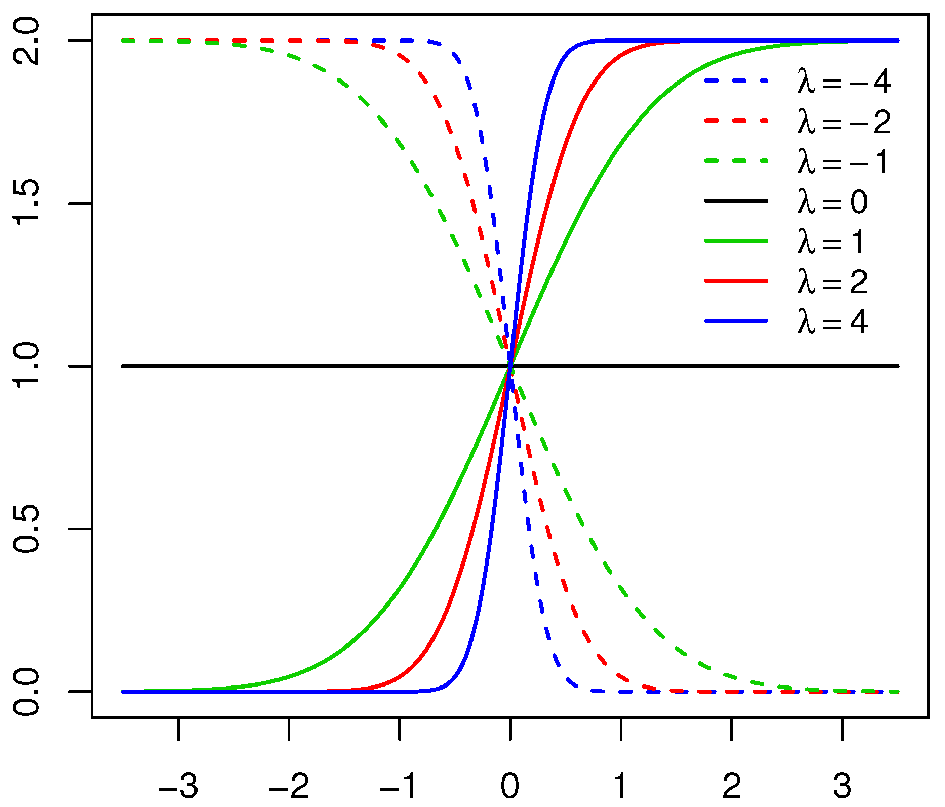
Consider a random variable with PDF defined in Definition 1. The behavior of the skewing mechanism and the PDF of the distribution is illustrated in Figure 1 and Figure 2, respectively (for specific parameter structures). From Definition 1, it is clear that does not affect the skewing mechanism, as opposed to . When , the skewing mechanism yields a value of one, and the distribution simplifies to the symmetric distribution. Furthermore, as the absolute value of increases, the range of x values over which the skewing mechanism is applied decreases within the interval . As a result, higher peaks are evident in the PDF of the distribution [11]. These properties are illustrated in Figure 1 and Figure 2.
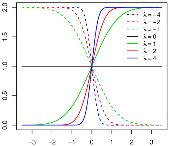
Figure 1.
Skewing mechanism for the skew generalized normal () distribution with , , , and various values of .
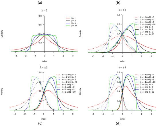
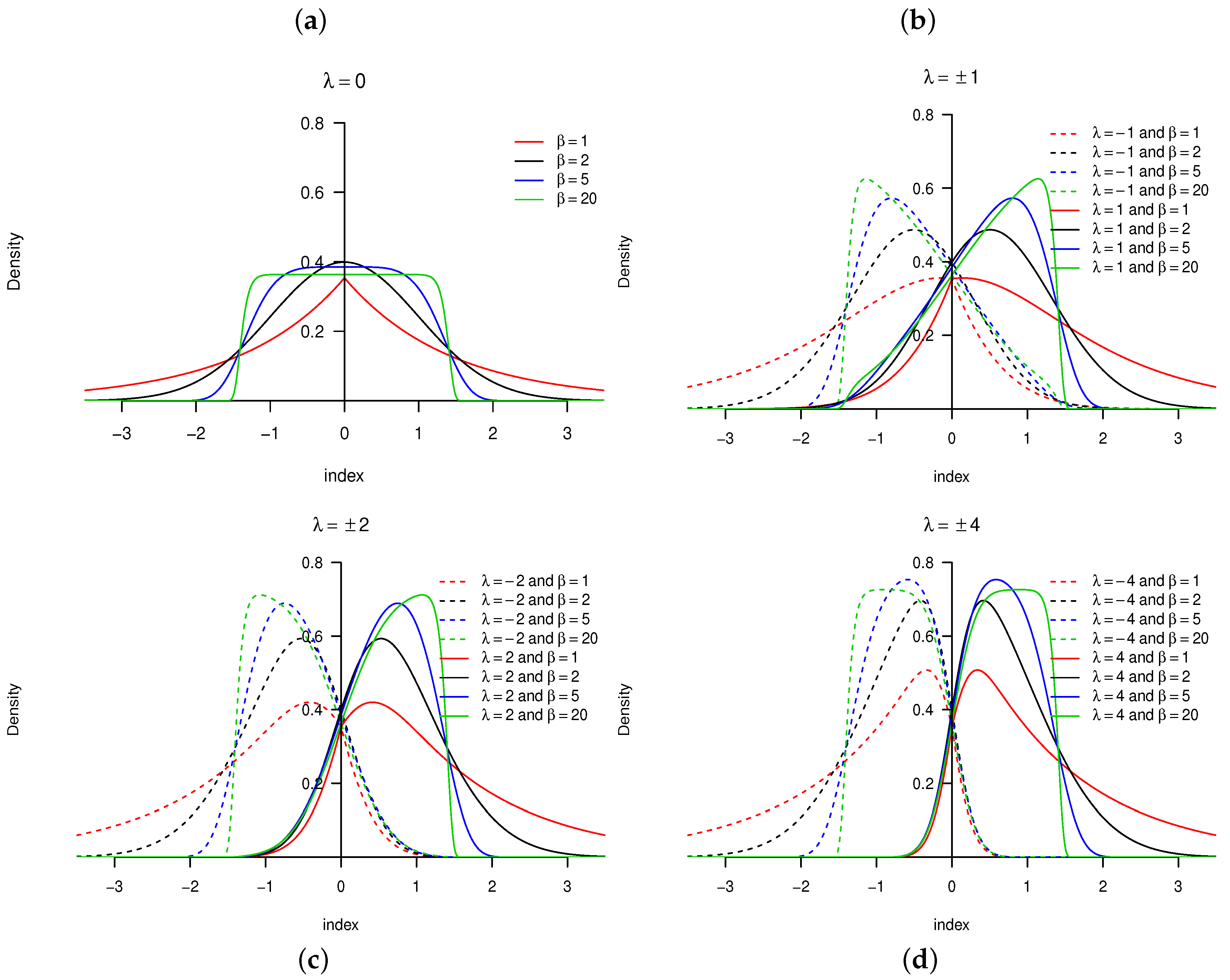
Figure 2.
Probability density function (PDF) for the distribution with , and various values of for (from left to right, top to bottom): (a) ; (b) ; (c) ; (d) .
The main advantage of the distribution is its flexibility by accommodating both skewness and kurtosis (specifically, heavier tails than that of the distribution); the reader is referred to [11] for more detail. Furthermore, a random variable from the binomial distribution with parameters n and p can be approximated by a normal distribution with mean and variance if n is large or (that is, when the distribution is approximately symmetrical). However, if , an asymmetric distribution is observed with considerable skewness for both large and small values of p. Bekker et al. [9] addressed this issue and showed that the distribution outperforms both the normal and distributions in approximating binomial distributions for both large and small values of p with .
In order to demonstrate some characteristics (in particular, the expected value, variance, kurtosis, skewness, and moment generating function (MGF)) of the distribution, the following theorem from [11] can be used to approximate the kth moment.
Theorem 1.
Suppose with the PDF defined in Definition 1 for and , then:
where A is a random variable distributed according to the gamma distribution with scale and shape parameters 1 and , respectively.
Proof.
The reader is referred to [11] for the proof of Theorem 1. □
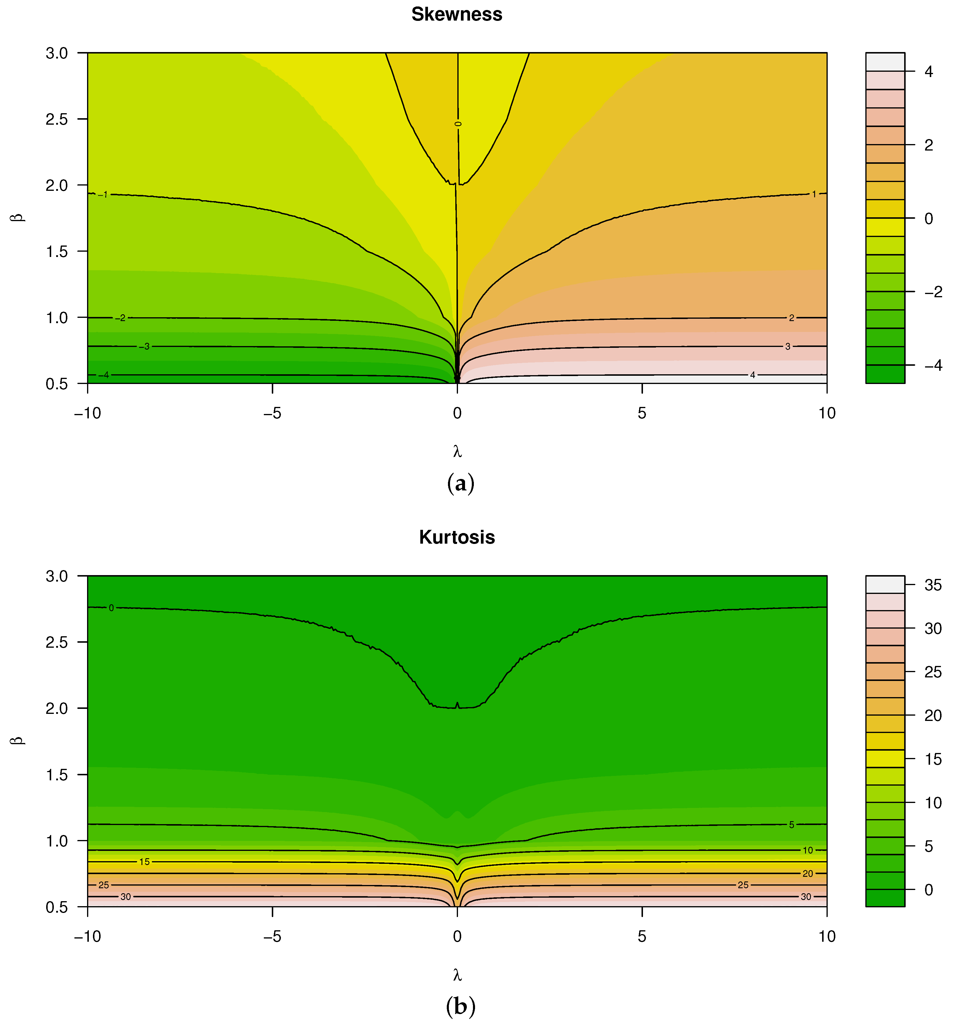
Theorem 1 is shown to be the most stable and efficient for approximating the kth moment of the distribution of X, although it is also important to note that the sample size such that significant estimates of these characteristics are obtained. Figure 3 illustrates the skewness and kurtosis characteristics that were calculated using Theorem 1 for various values of and . When evaluating these characteristics, it is seen that both kurtosis and skewness are affected by and jointly. In particular (referring to Figure 3):

Figure 3.
Measures for for various values of and (from top to bottom): (a) Skewness. (b) Kurtosis.
- Skewness is a monotonically increasing function for —that is, for , the distribution is negatively skewed, and vice versa.
- In contrast to the latter, skewness is a non-monotonic function for .
- Considering kurtosis, all real values of and decreasing values of result in larger kurtosis, yielding heavier tails than that of the normal distribution.
In a more general sense for an arbitrary and , Theorem 1 can be extended as follows:
Theorem 2.
Suppose and such that , then:
with defined in Theorem 1.
Proof.
The proof follows from Theorem 1 [11]. □
Theorem 3.
Suppose with the PDF defined in Definition 1 for and , then the MGF is given by:
where W is a random variable distributed according to the generalized gamma distribution (refer to [11] for more detail) with scale, shape, and generalizing parameters 1, , and β, respectively.
Proof.
From Definition 1 and (2), it follows that:
Furthermore, using the infinite series representation of the exponential function:
where W is a random variable distributed according to the generalized gamma distribution with scale, shape, and generalizing parameters 1, and , respectively, and PDF:
when , and zero otherwise. Similarly, can be written as:
Thus, the MGF of X can be written as follows:
□
The representation of the MGF (and by extension, the characteristic function) of the distribution, defined in Theorem 3 above, can be seen as an infinite series of weighted expected values of generalized gamma random variables.
Remark 1.
It is clear that β and λ jointly affect the shape of the distribution. In order to distinguish between the two parameters, this paper will refer to λ as the skewing parameter, since the skewing mechanism depends on λ only. β will be referred to as the generalization parameter, as it accounts for flexibility in the tails and generalizing the normal to the distribution of [13].
3. The ARSGN() Model and Its Estimation Procedure
This section focuses on the model definition and ML estimation procedure of the ARSGN(p) model.
Definition 2.
If is defined by an AR(p) process with independent innovations with PDF:
then it is said that is defined by an ARSGN(p) process for time and with process mean .
Remark 2.
The process mean for an AR(p) process keeps its basic definition, regardless of the underlying distribution for the innovation process .
With representing the process of independent distributed innovations with the PDF defined in Definition 2, the joint PDF for is given as:
for . Furthermore, from (1), the innovation process can be rewritten as:
Since the distribution for is intractable (being a linear combination of variables), the complete joint PDF of is approximated by the conditional joint PDF of , for , which defines the likelihood function for the ARSGN(p) model. Thus, using (3) and (4), the joint PDF of given is given by:
where . The ML estimator is based on maximizing the conditional log-likelihood function, where . Evidently, the parameters need to be estimated for an AR(p) model, where m represents the number of parameters in the distribution considered for the innovation process.
Theorem 4.
If is characterized by an ARSGN(p) process, then the conditional log-likelihood function is given as:
for and defined in Definition 2.
The conditional log-likelihood in Theorem 4 can be written as:
where and is defined in (4). The ML estimation process of the ARSGN(p) process is summarized in Algorithm 1 below.
| Algorithm 1: |
|
4. Application
In this section, the performance and robustness of the ML estimator for the ARSGN(p) time series model is illustrated through various simulation studies. The proposed model is also applied to real data in order to illustrate its relevance, in comparison to previously proposed models. All computations were carried out using in a Win 64 environment with a 2.30 GHz/Intel(R) Core(TM) i5-6200U CPU Processor and 4.0 GB RAM, and run times are given in seconds. The code is available from the first author upon request.
4.1. Numerical Studies
The aim of this subsection is to illustrate the performance and robustness of the conditional ML estimator for the proposed model in Definition 2 using various simulation studies. Define the hypothetical AR(5) time series model, which will (partly) be considered in the simulation studies below:
where and the sample size n will be defined differently for each simulation study. The simulation studies are algorithmically described in Algorithm 2 below.
| Algorithm 2: |
|
4.1.1. Simulation Study 1
In order to evaluate the conditional ML estimation performance of the ARSGN(p) model, the time series will be simulated and estimated for various orders of and sample sizes . Assuming for the hypothetical model defined in (6), the innovation process is simulated and the time series is estimated with an ARSGN(p) model, as described in Algorithm 2.
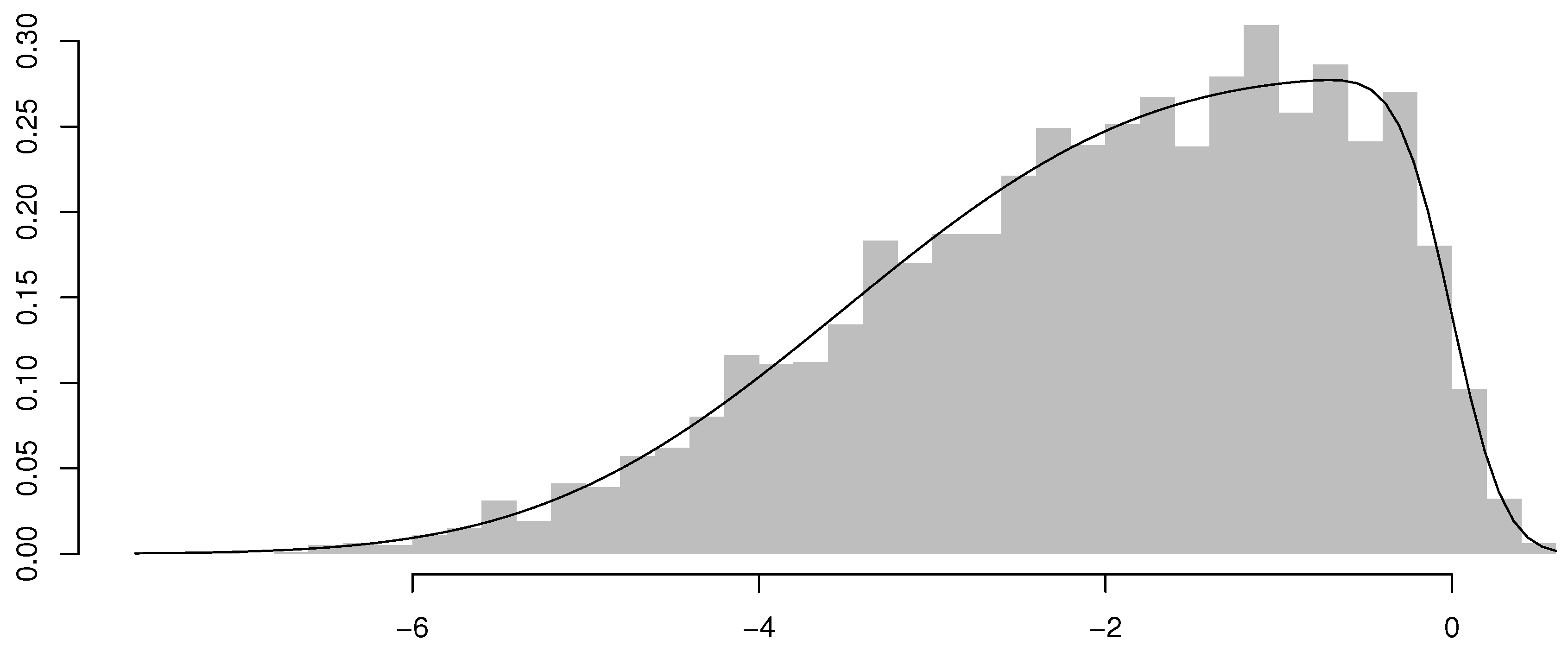
Table 1 summarizes the parameter estimates and standard errors obtained from the ARSGN(p) model for all and . In general, it is clear that the model fits the simulated innovation processes (and time series) relatively well, except for , which tends to be more volatile with larger standard errors, although these standard errors decrease for larger sample sizes. It is also noted that there are occasional trade-offs in the estimation of and for and , which decreases the standard error for one parameter, but increases the standard error of the other. These occasional instances of “incorrect” estimations, which consequently have an influence on the estimation of as well, may be explained by the fact that and are jointly affecting the asymmetric behavior in the distribution. In addition to Table 1, Figure 4 illustrates the estimated ARSGN(3) model with the distribution of the residuals, where the residual at time t is defined as:
and representing the estimated value at time t. The asymmetric behavior of the distribution is especially seen from the fitted model in Figure 4.

Table 1.
The autoregressive (AR) process of order p using the skew generalized normal (ARSGN(p)) maximum likelihood (ML) parameter estimates and standard errors (in parentheses) for various sample sizes n and values of p.

Figure 4.
Histogram of the residuals with the fitted ARSGN(3) model overlaid for sample size .
4.1.2. Simulation Study 2
Sampling distributions for the parameters can be used to evaluate the robustness of the estimator for the proposed model. In order to construct the sampling distributions for the parameters in Table 1, a Monte Carlo simulation study is applied by repeating the simulation for and the estimation procedure 500 times, considering and for the hypothetical model defined in (6) with .
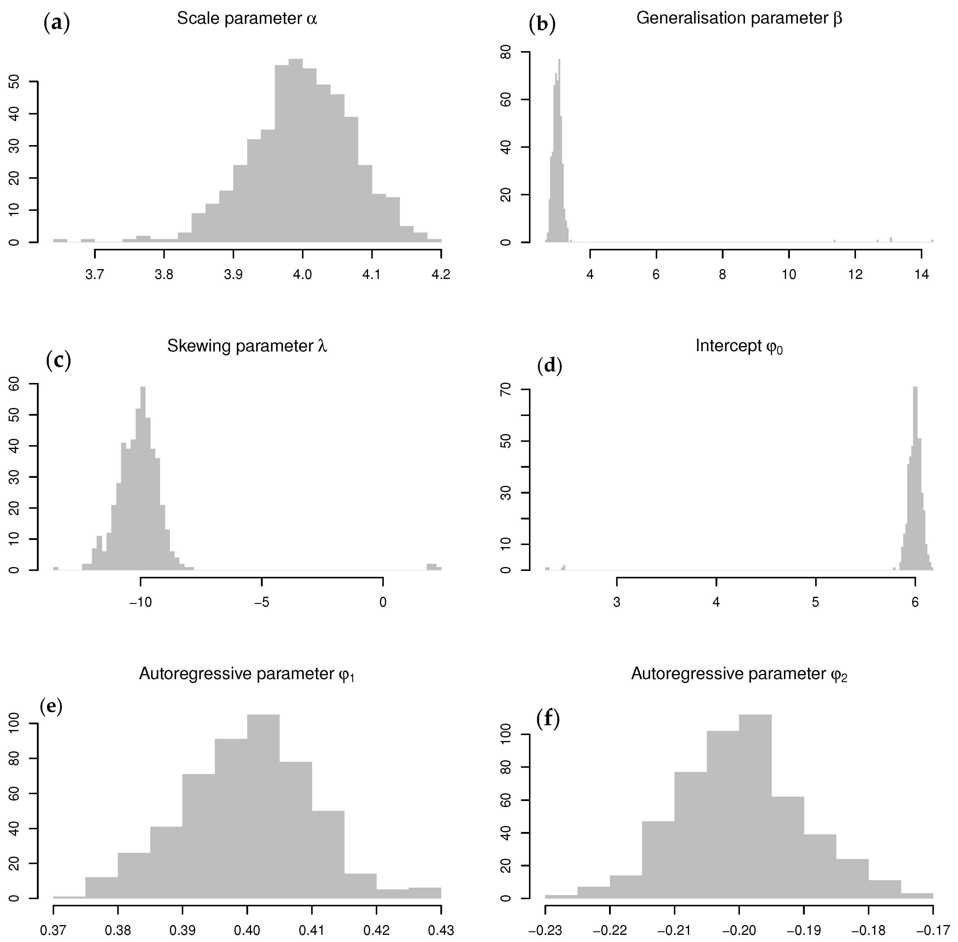
The sampling distributions obtained for the conditional ML parameter estimates are illustrated in Figure 5, all centered around their theoretical values. The occasional trade-offs between and (noted in Simulation Study 1) are evident from these distributions. Furthermore, Table 2 summarizes the 5th, 50th (thus, the median), and 95th percentiles obtained from these sampling distributions, of which the 5th and 95th percentiles can be used for approximating the 95% confidence intervals. It is evident that the theoretical values for all parameters fall within their respective 95% confidence intervals and exclude zero, suggesting that all parameter estimates are significant. It is concluded that the conditional ML estimation of the proposed model is robust since all 50th percentiles are virtually identical to each of the theoretical values, confirming what is depicted in Figure 5.

Figure 5.
Sampling distributions for the ARSGN(2) ML parameter estimates obtained from a Monte Carlo simulation study (from left to right, top to bottom): (a) Sampling distribution for . (b) Sampling distribution for . (c) Sampling distribution for . (d) Sampling distribution for . (e) Sampling distribution for . (f) Sampling distribution for .
Table 2.
Percentiles for the ARSGN(2) ML parameter estimates obtained from a Monte Carlo simulation study.
4.1.3. Simulation Study 3
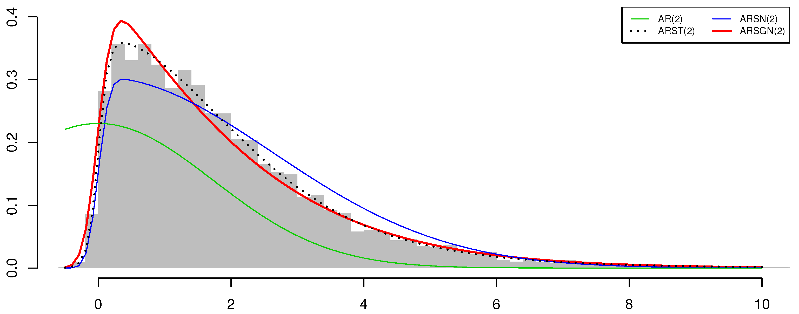
For comparison and completeness’ sake, consider the hypothetical time series model defined in (6), for up to only. This time, the innovation process is simulated from an distribution such that [12], and thus, the simulated time series is referred to as an ARST(2) process. The aim of this simulation study is to evaluate the fit of the ARSGN(2) model in comparison to the AR(2), ARSN(2), and ARST(2) models each, even though the true innovation process follows an distribution.
Considering a sample size of , the innovation process was simulated using the rst() function in . The AR(2), ARSN(2), ARSGN(2), and ARST(2) models are each fitted to the time series by maximizing the respective conditional log-likelihood functions. Starting values were chosen similar for all models as discussed in Algorithm 1, except for , being set equal to the sample skewness for both the ARSN(2) and ARST(2) models and the degrees of freedom being initialized at one for the latter. It should be noted that the starting value for in the ARSGN(p) model was not set to the sample skewness, since it was noted in Section 2 that and jointly affect the skewness and shape of the distribution.
Table 3 summarizes the conditional ML parameter estimates with the standard errors given in parentheses, as well as the log-likelihood, Akaike information criterion (AIC), and run times for the various AR models, where AIC is defined as:
with representing the maximized value of the log-likelihood function defined in Theorem 4 and M denoting the number of parameters in the model [16]. From the log-likelihood and AIC values obtained for the different models, it can be seen that the ARSGN(2) model competes well with the ARST(2) model (see Figure 6). In particular, the run time for the estimation of the ARSGN(2) model is shorter than that of the ARST(2) model, with all parameters being significant at a 95% confidence level. Thus, it can be concluded that the ARSGN(2) model is a valid contender in comparison to other popular models accounting for asymmetry, kurtosis, and heavy tails and performs competitively considering the computational time.
Table 3.
AR(2) ML parameter estimates with standard errors (in parentheses), log-likelihood , Akaike information criterion (AIC), and run times for sample size and . ST, skew-t.
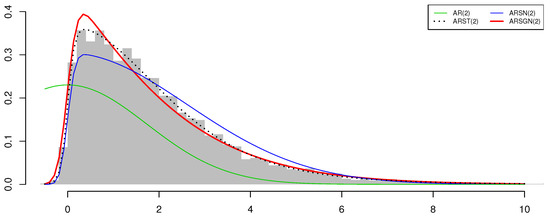
Figure 6.
Histogram of simulated innovation process with fitted AR(2) models overlaid for sample size .
4.1.4. Simulation Study 4
The purpose of this simulation study is to evaluate the estimation performance and adaptability of the proposed ARSGN(p) model (in comparison to some of its competitors) on processes with various tail weights simulated from the distribution. Thus, consider the hypothetical time series model defined in (6), for up to only and with where represents the different degrees of freedom under which will be simulated. For a sample size of n = 10,000, the AR(2) model is estimated assuming various distributions for the innovation process .
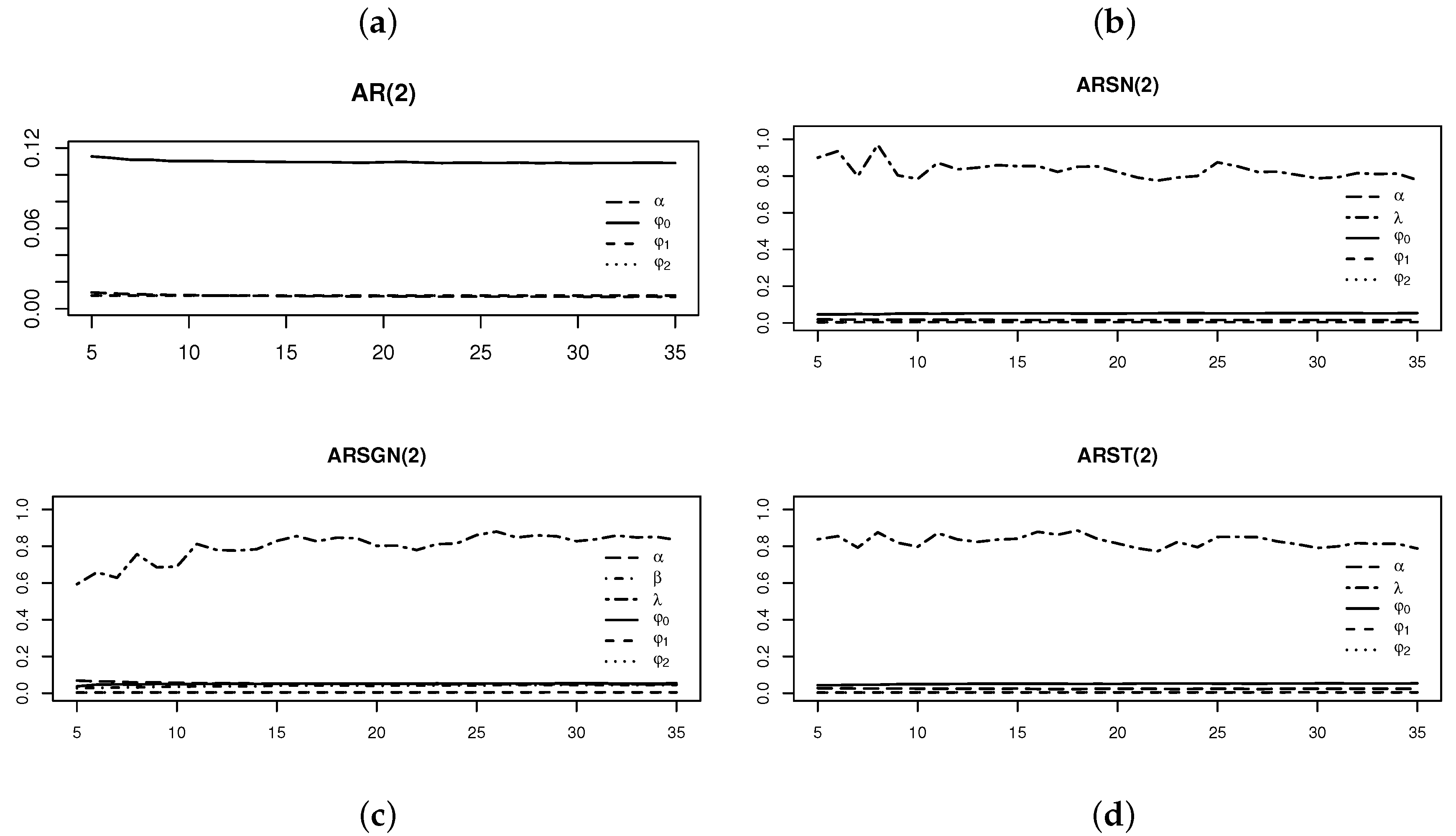
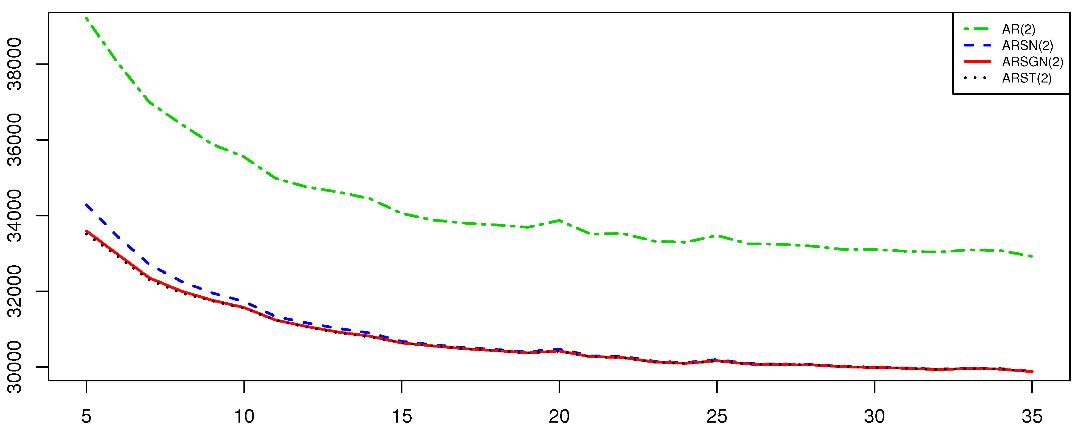
Figure 7 and Figure 8 illustrate the standard errors of the estimates of the parameters of interest and AIC values obtained from the various AR models fitted to the simulated ARST(2) process for degrees of freedom . Figure 7 illustrates that the skewing parameter for the ARSGN(2) model is more volatile compared to the other parameters, although it performs with less volatility than in the ARSN(2) model for lower degrees of freedom. Observing the AIC values in Figure 8, it is clear that the AR(2) model (under the assumption of normality) performs the worst for all degrees of freedom, whereas the ARSN(2) model performs similar to that of the ARST(2) for degrees of freedom . In contrast, the proposed ARSGN(2) model performs almost equivalently to the ARST(2) model for all degrees of freedom indicating that the proposed model adapts well to various levels of skewness and kurtosis.

Figure 7.
Standard errors of the parameter estimates obtained from AR(2) models fitted to an ARST(2) process simulated with for different degrees of freedom . From left to right, top to bottom: (a) AR(2) model fitted assuming . (b) AR(2) model fitted assuming . (c) AR(2) model fitted assuming . (d) AR(2) model fitted assuming .
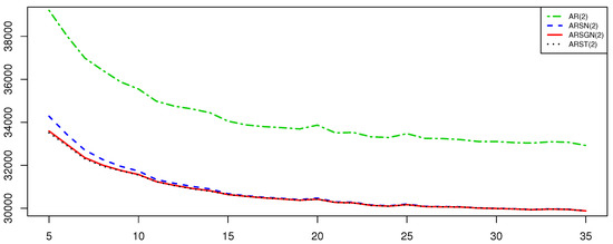
Figure 8.
AIC values obtained from AR(2) models fitted (assuming various distributions for ) to an ARST(2) process simulated with for different degrees of freedom .
4.2. Real-World Time Series Analysis
This subsection illustrates the relevance of the ARSGN(p) model in areas such as chemistry, population studies, and economics, in comparison to previously proposed AR models. Descriptive statistics for all time series considered below are summarized in Table 4.
Table 4.
Descriptive statistics of real time series data considered below, where * refers to the stationary time series data.
4.2.1. Viscosity during a Chemical Process
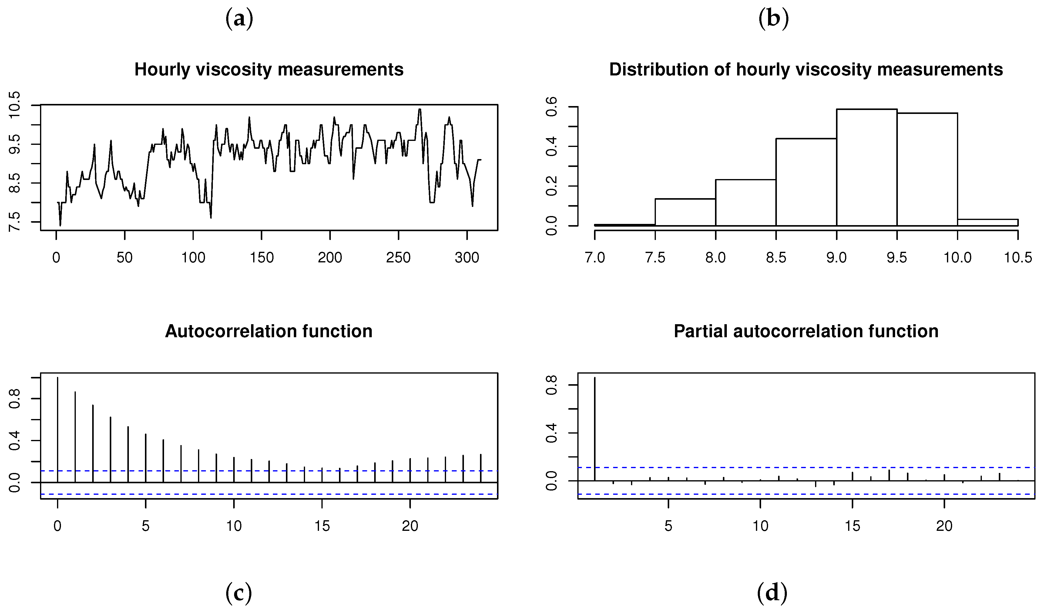
In order to compare the ARSGN(p) model, defined in Definition 2, to previously proposed models (i.e., AR models assuming the normal and distributions for the innovation process , respectively), consider the time series data Series D in [17]. This dataset consists of hourly measurements of viscosity during a chemical process, represented in Figure 9. The Shapiro–Wilk test applied to the time series data suggests that the data are not normally distributed with a p-value ; this is also confirmed by the histogram in Figure 9. From the autocorrelation function (ACF) and partial autocorrelation function (PACF), it is evident that an AR(1) model is a suitable choice for fitting a time series model.
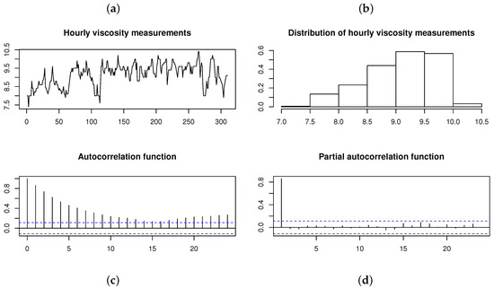
Figure 9.
Viscosity measured hourly during a chemical process [17]. From left to right, top to bottom: (a) Time plot. (b) Histogram. (c) Autocorrelation function (ACF). (d) Partial autocorrelation function (PACF).
Previously, Box and Jenkins [17] fit an AR(1) model to this time series, assuming that the innovations are normally distributed. Sharafi and Nematollahi [6] relaxed this normality assumption and allowed for asymmetry by fitting an ARSN(1) model. Table 5 summarizes the conditional ML parameter estimates (with the standard errors given in parentheses) for both of these models, together with those obtained for the newly proposed ARSGN(1) model and the ARST(1) model. In addition, the maximized log-likelihood, AIC values, Kolmogorov–Smirnov (KS) test statistics, and run times are also represented for the various models, where the KS test statistic is defined as:
where and represent the empirical and estimated distribution functions for the residuals and innovation process, respectively [18]. From the log-likelihood, AIC values, and KS test statistics calculated for the four models, it can be concluded that the ARSGN(1) model fits this time series the best, with a competitive estimation run time. Take note that from the estimated intercept , the process mean is estimated as , which is evident from the time plot in Figure 9.
Table 5.
ML parameter estimates with standard errors (in parentheses), log-likelihood , AIC, Kolmogorov–Smirnov (KS) test statistics, and run times for the hourly viscosity measurements during a chemical process [17].
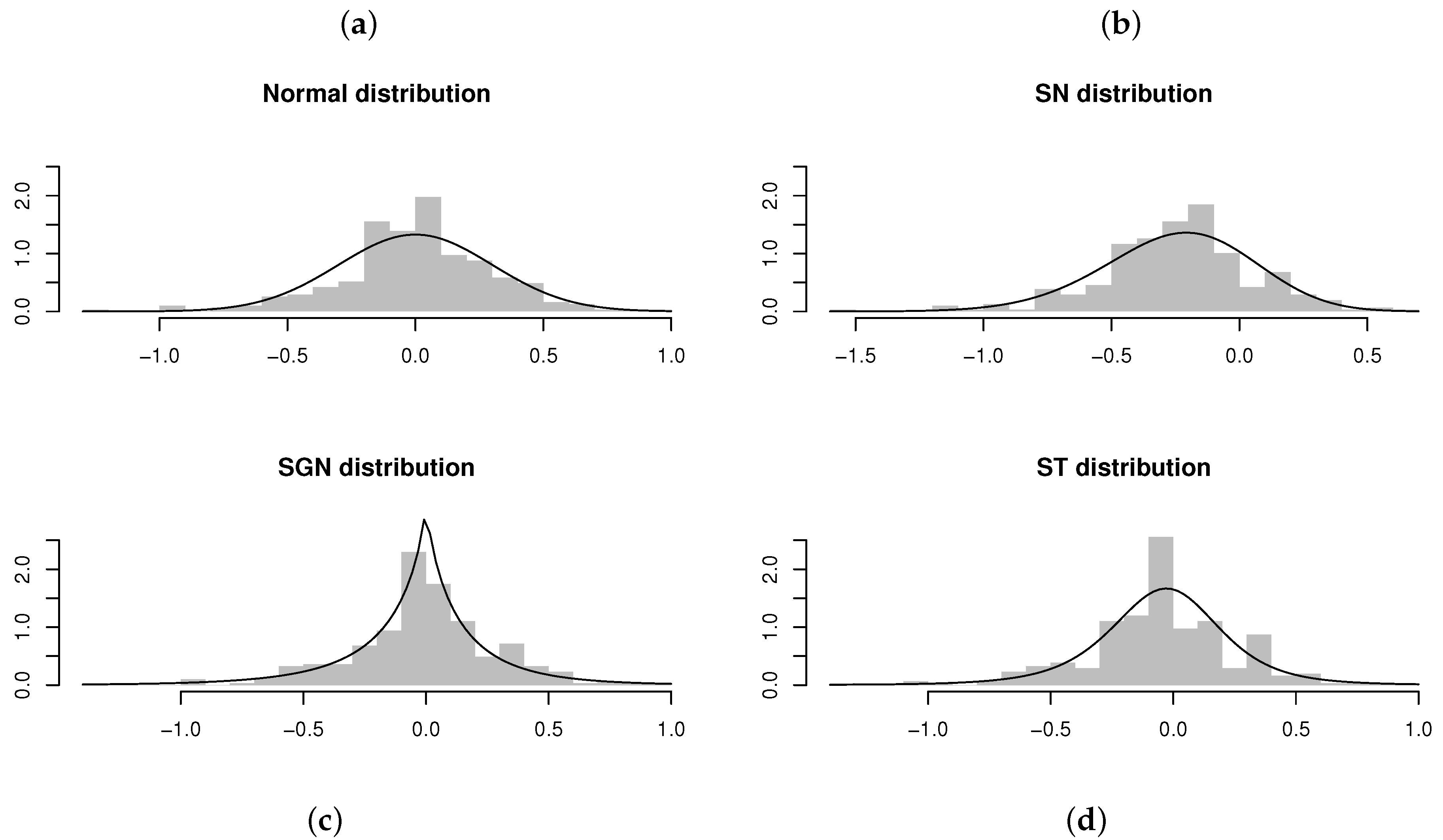
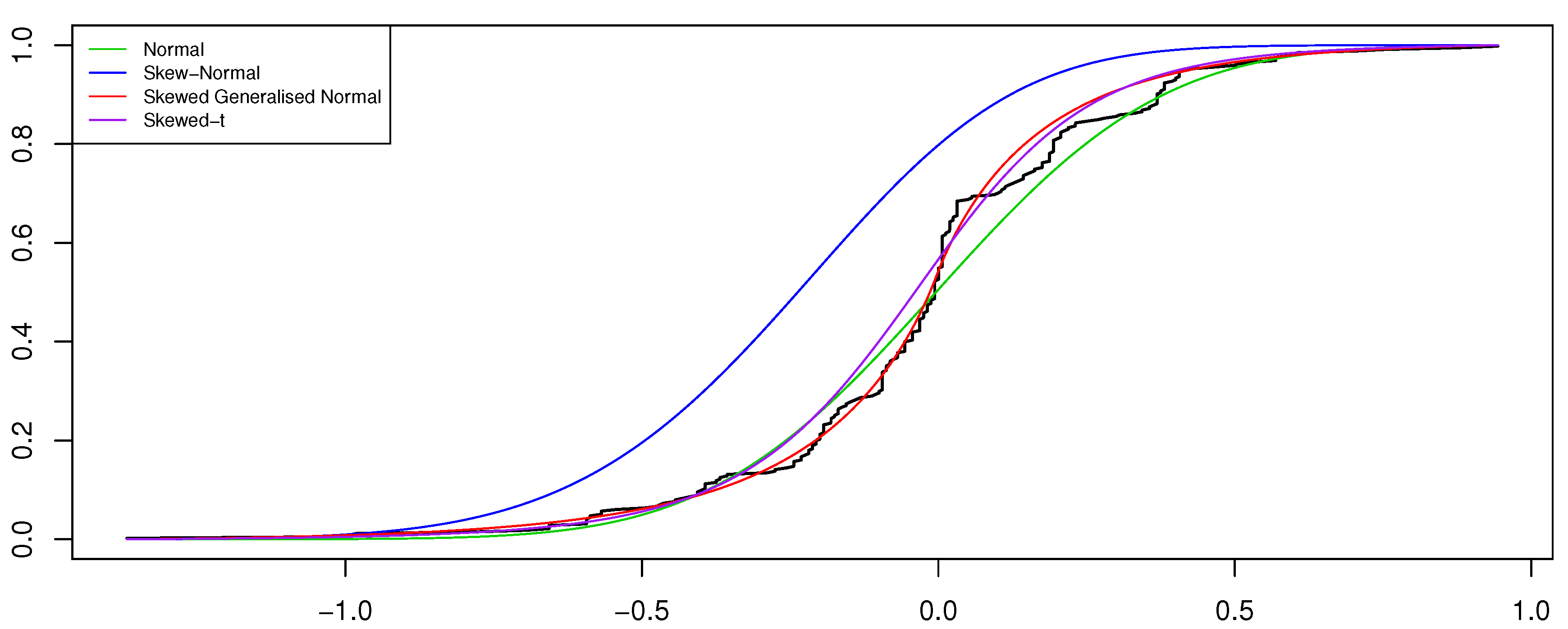
Evaluating the standard errors for the parameter estimates obtained for the ARSGN(1) model, it is observed that all parameters differ significantly from zero at a 95% confidence level, except for the skewing parameter , suggesting that the innovation process does not contain significant skewness. This is confirmed by Figure 10, from which it is clear that only slight skewness is present when observing the distribution for the residuals obtained for all four models. In this case, it is also clear to see that the distribution captures the kurtosis well. Finally, Figure 11 illustrates the CDFs for the various estimated models together with the empirical CDFs for the residuals obtained from the ARSGN(1) model, suggesting that the ARSGN(1) model fits the innovation process best.

Figure 10.
Residuals and estimated models obtained from AR(1) models fitted to the viscosity time series [17]. From left to right, top to bottom: (a) AR(1) model fitted assuming . (b) AR(1) model fitted assuming . (c) AR(1) model fitted assuming . (d) AR(1) model fitted assuming .
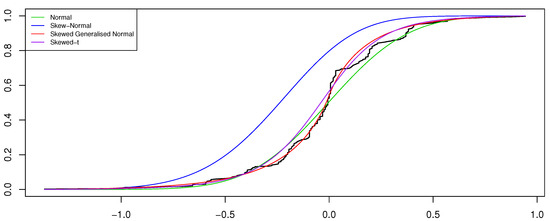
Figure 11.
Cumulative distribution function (CDF) for the estimated AR(1) models under various distributions assumed for the innovation process , with the empirical CDF for the residuals obtained from the estimated ARSGN(1) model for the viscosity time series [17].
4.2.2. Estimated Resident Population for Australia
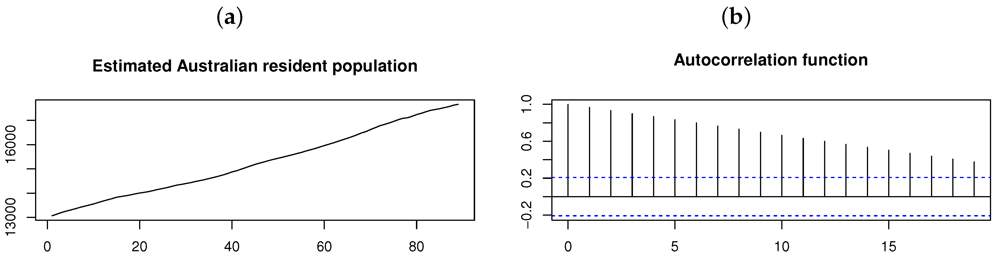
In order to illustrate the relevance of the proposed model for higher orders of p, consider the quarterly estimated Australian resident population data (in thousands), which consists of observations from June 1971 to June 1993. Figure 12 shows the time plot and ACF for the original time series from which it is clear that nonstationarity is present since the process mean and autocorrelations depend on time. This is also confirmed by the augmented Dickey–Fuller (ADF) test, which yields a p-value , suggesting that the time series exhibits a unit root [19].
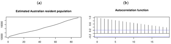
Figure 12.
Australian resident population on a quarterly basis from June 1971 to June 1993 (estimated in thousands). From left to right: (a) Time plot. (b) ACF.
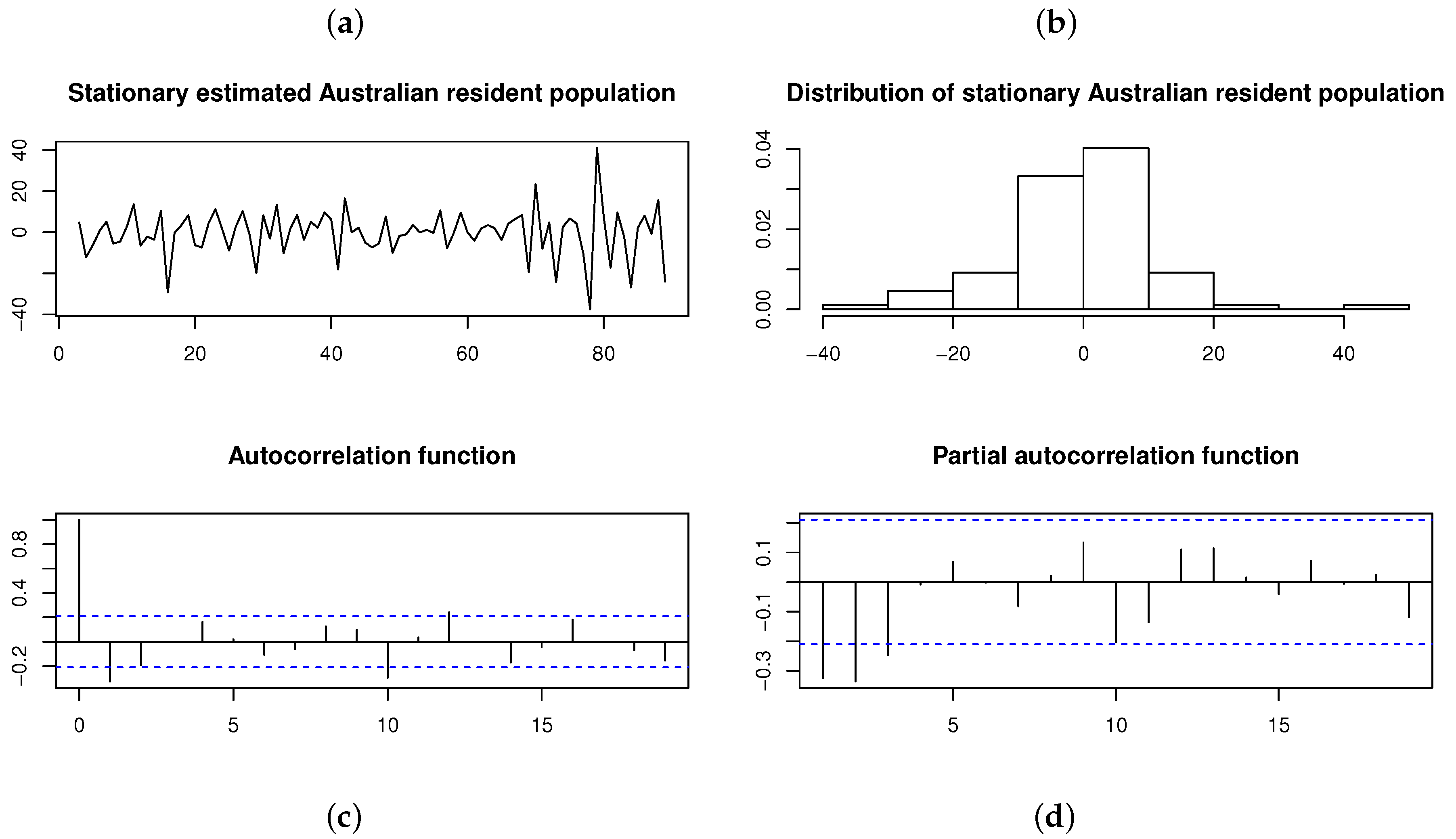
Transforming the original time series by differencing the time series twice yields a stationary time series with a p-value for the ADF test (suggesting no unit roots). This stationary time series and its distribution are illustrated in Figure 13, with the ACF and PACF suggesting that an AR(3) model is the appropriate choice for fitting a time series model. Previously, Brockwell and Davis [20] fitted an AR(3) model to the differenced (i.e., stationary) time series, assuming that the innovations are normally distributed. However, both the histogram and Shapiro–Wilk test (with p-value ) applied to this stationary time series suggest that the innovation process is not normally distributed. Instead, is considered as a distribution for the innovation process—that is, .
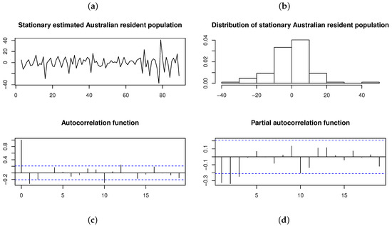
Figure 13.
Differenced (i.e., stationary) Australian resident population on a quarterly basis from June 1971 to June 1993 (estimated in thousands). From left to right, top to bottom: (a) Time plot. (b) Histogram. (c) ACF. (d) PACF.
Table 6 summarizes the estimation results for AR models under the distribution in comparison to the normal, , and distributions. From the maximized log-likelihood, AIC values, and KS test statistics calculated for the four models, it can be concluded that the ARSGN(3) model fits the best, with an estimated process mean (also evident from Figure 13). Furthermore, evaluating the standard errors of the parameters obtained for the ARSGN(3) model, it is evident that all parameters differ significantly from zero at a 95% confidence level, except for the skewing parameter , suggesting that the innovation process does not exhibit significant skewness. Figure 14 illustrates these estimated models, confirming that the proposed ARSGN(3) model adapts well to various levels of asymmetry.
Table 6.
ML parameter estimates with standard errors (in parentheses), log-likelihood , AIC, KS test statistics, and run times for the differenced time series of estimated Australian resident population on a quarterly basis from June 1971 to June 1993.
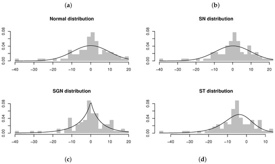
Figure 14.
Residuals and estimated models obtained from AR(3) models fitted to the differenced time series of the estimated Australian resident population on a quarterly basis (from June 1971 to June 1993). From left to right, top to bottom: (a) AR(3) model fitted assuming . (b) AR(3) model fitted assuming . (c) AR(3) model fitted assuming . (d) AR(3) model fitted assuming .
4.2.3. Insolvencies in South Africa
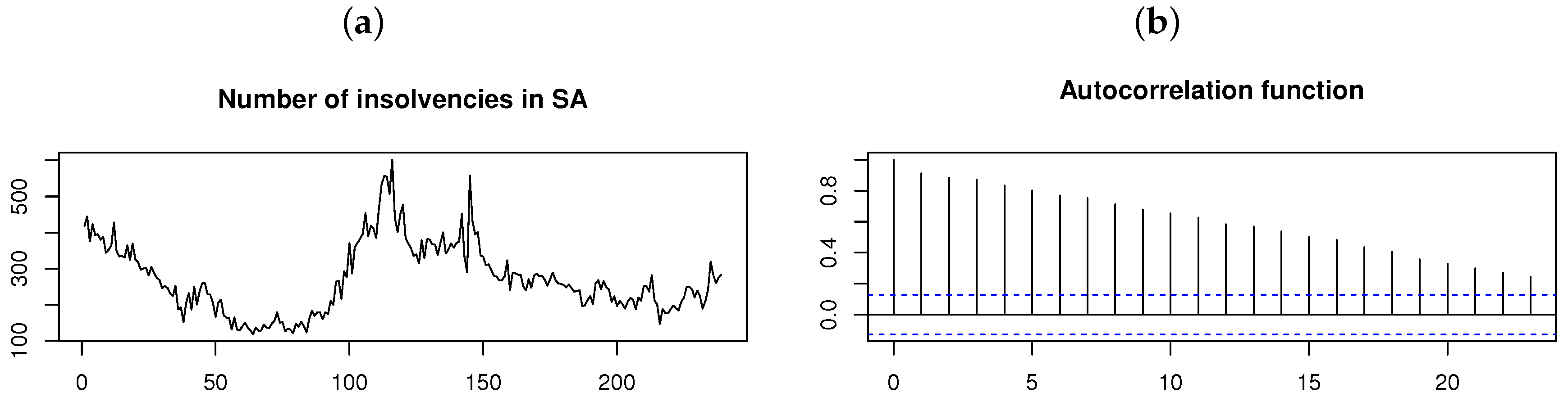
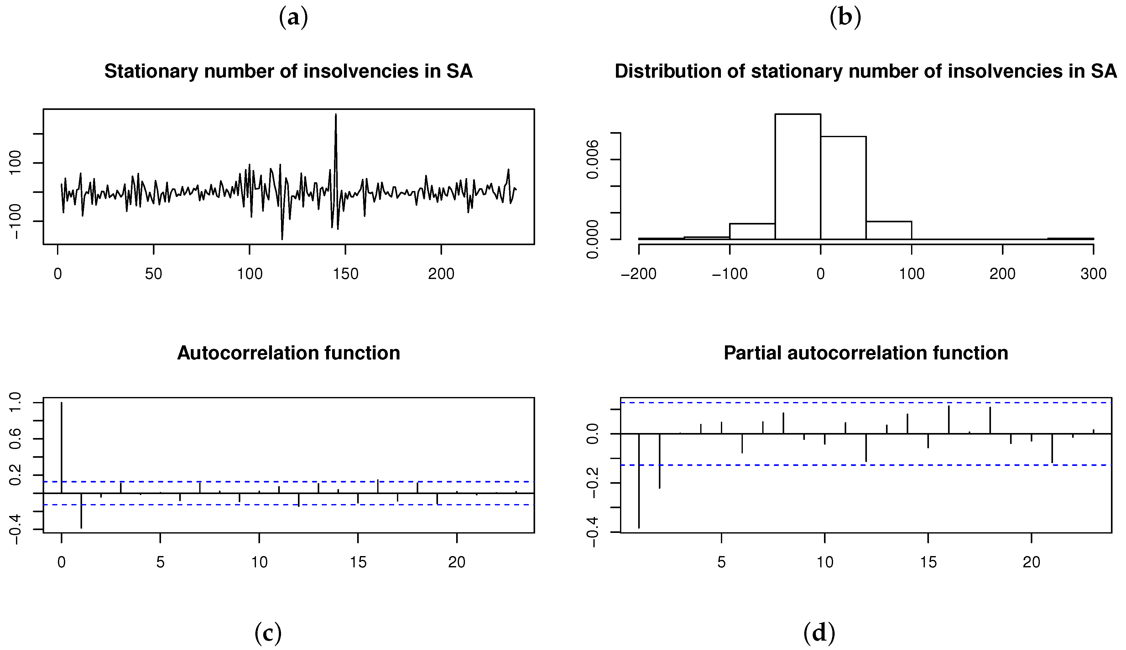
As a final application, consider the monthly (seasonally adjusted) number of insolvencies in South Africa for January 2000 to November 2019 (retrieved from Stats SA [21]). The time plot and ACF for the time series in Figure 15 suggests that the time series is nonstationary (which is also confirmed by the ADF test with p-value ). A stationary time series is obtained by differencing the original time series once. This stationary time series and its distribution is illustrated in Figure 16, with the ACF and PACF suggesting that an AR(2) model is the appropriate choice for fitting a time series model. Although the Shapiro–Wilk test yields a p-value (suggesting non-normality), the AR(2) model is fitted assuming each of the normal, , , and distributions for the innovation process , respectively; Table 7 and Figure 17 show the results obtained.
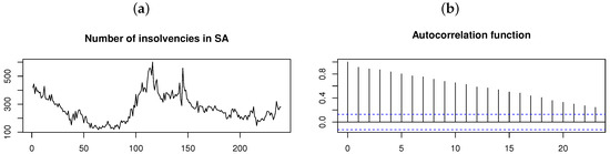
Figure 15.
Number of insolvencies per month in South Africa from January 2000 to November 2019 [21]. From left to right: (a) Time plot. (b) ACF.
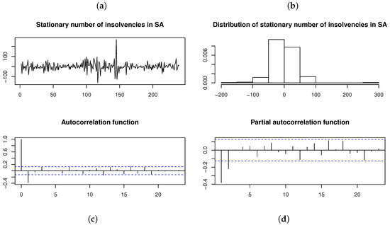
Figure 16.
Differenced (i.e., stationary) number of insolvencies per month in South Africa from January 2000 to November 2019 [21]. From left to right, top to bottom: (a) Time plot. (b) Histogram. (c) ACF. (d) PACF.
Table 7.
ML parameter estimates with standard errors (in parentheses), log-likelihood , AIC, KS test statistics, and run times for the differenced time series of number of insolvencies per month in South Africa from January 2000 to November 2019 [21].
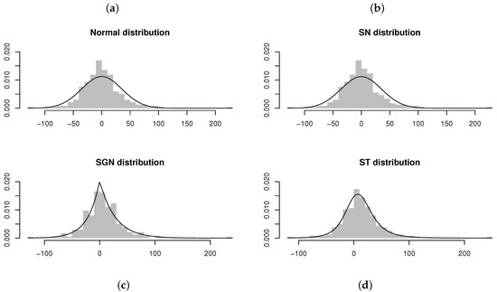
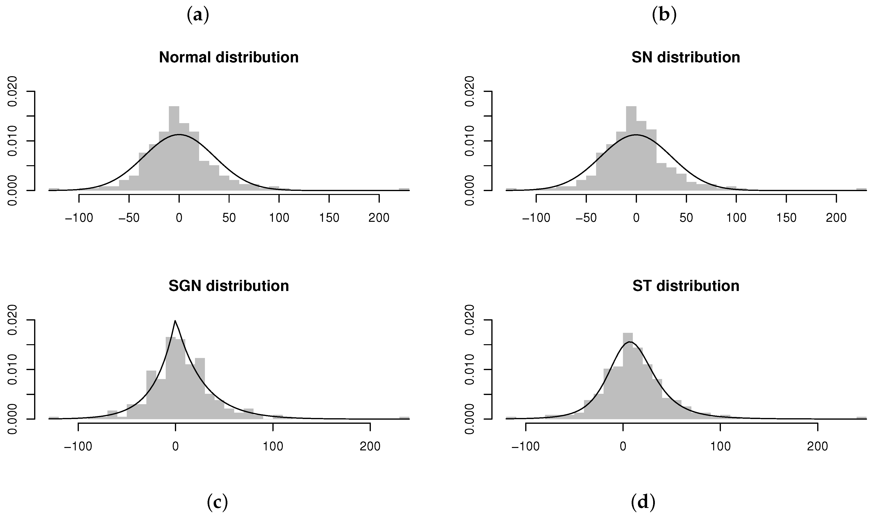
Figure 17.
Residuals and estimated models obtained from AR(2) models fitted to the differenced time series of number of insolvencies per month in South Africa (from January 2000 to November 2019) [21]. From left to right, top to bottom: (a) AR(2) model fitted assuming . (b) AR(2) model fitted assuming . (c) AR(2) model fitted assuming . (d) AR(2) model fitted assuming .
Referring to Table 7, it appears as if the ARST(2) model fits the best, with the proposed ARSGN(2) model as the runner-up (by comparing the maximized log-likelihood and AIC values). However, when comparing the standard errors for the parameter estimates, it is suggested that the estimates for the ARSGN(2) model generally exhibit less volatility compared to its competitors, with all parameters being significant at a 95% confidence level. Figure 17 confirms that the distribution adapts well to various levels of skewness and kurtosis.
5. Conclusions
In this paper, the AR(p) time series model with skewed generalized normal () innovations was proposed, i.e., ARSGN(p). The main advantage of the distribution is its flexibility by accommodating asymmetry, kurtosis, as well as heavier tails than the normal distribution. The conditional ML estimator for the parameters of the ARSGN(p) model was derived and the behavior was investigated through various simulation studies, in comparison to previously proposed models. Finally, real-time series datasets were fitted using the ARSGN(p) model, of which the usefulness was illustrated by comparing the estimation results for the proposed model to some of its competitors. In conclusion, the ARSGN(p) is a meaningful contender in the AR(p) environment compared to other often-considered models. A stepping-stone for future research includes the extension of the ARSGN(p) model for the multivariate case. Furthermore, an alternative method for defining the non-normal AR model by discarding the linearity assumption may be explored; see, for example, the work done on non-linear time series models in [22,23].
Author Contributions
Conceptualization, J.F. and M.N.; methodology, A.N., J.F., A.B., and M.N.; software, A.N.; formal analysis, A.N.; investigation, A.N.; writing, original draft preparation, A.N.; writing, review and editing, A.N., J.F., A.B., and M.N.; visualization, A.N.; supervision, J.F. and M.N.; funding acquisition, J.F. and A.B. All authors read and agreed to the published version of the manuscript.
Funding
This work was based on research supported by the National Research Foundation, South Africa (SRUG190308422768 nr. 120839), the South African NRF SARChI Research Chair in Computational and Methodological Statistics (UID: 71199), the South African DST-NRF-MRC SARChI Research Chair in Biostatistics (Grant No. 114613), and the Research Development Programme at UP 296/2019.
Acknowledgments
Hereby, the authors would like to acknowledge the support of the StatDisT group based at the University of Pretoria, Pretoria, South Africa. The authors also thank the anonymous reviewers for their comments, which improved the quality of the paper.
Conflicts of Interest
The authors declare no conflict of interest. The funders had no role in the design of the study; in the collection, analyses, or interpretation of data; in the writing of the manuscript; nor in the decision to publish the results.
References
- Pourahmadi, M. Foundation of Time Series Analysis and Prediction Theory; John Wiley & Sons, Inc.: Hoboken, NJ, USA, 2001. [Google Scholar]
- Pourahmadi, M. Stationarity of the solution of (Xt = AtXt−1+εt) and analysis of non-Gaussian dependent random variables. J. Time Ser. Anal. 1988, 9, 225–239. [Google Scholar] [CrossRef]
- Tarami, B.; Pourahmadi, M. Multi-variate t autoregressions: Innovations, prediction variances and exact likelihood equations. J. Time Ser. Anal. 2003, 24, 739–754. [Google Scholar] [CrossRef]
- Grunwald, G.K.; Hyndman, R.J.; Tedesco, L.; Tweedie, R.L. Theory & methods: Non-Gaussian conditional linear AR(1) models. Aust. N. Z. J. Stat. 2000, 42, 479–495. [Google Scholar]
- Bondon, P. Estimation of autoregressive models with epsilon-skew-normal innovations. J. Multivar. Anal. 2009, 100, 1761–1776. [Google Scholar] [CrossRef]
- Sharafi, M.; Nematollahi, A. AR(1) model with skew-normal innovations. Metrika 2016, 79, 1011–1029. [Google Scholar] [CrossRef]
- Ghasami, S.; Khodadadi, Z.; Maleki, M. Autoregressive processes with generalized hyperbolic innovations. Commun. Stat. Simul. Comput. 2019, 1–13. [Google Scholar] [CrossRef]
- Tuaç, Y.; Güney, Y.; Arslan, O. Parameter estimation of regression model with AR(p) error terms based on skew distributions with EM algorithm. Soft Comput. 2020, 24, 3309–3330. [Google Scholar] [CrossRef]
- Bekker, A.; Ferreira, J.; Arashi, M.; Rowland, B. Computational methods applied to a skewed generalized normal family. Commun. Stat. Simul. Comput. 2018, 1–14. [Google Scholar] [CrossRef]
- Azzalini, A. A class of distributions which includes the normal ones. Scand. J. Stat. 1985, 12, 171–178. [Google Scholar]
- Rowland, B.W. Skew-Normal Distributions: Advances in Theory with Applications. Master’s Thesis, University of Pretoria, Pretoria, South Africa, 2017. [Google Scholar]
- Jones, M.; Faddy, M. A skew extension of the t-distribution, with applications. J. R. Stat. Soc. Ser. B Stat. Methodol. 2003, 65, 159–174. [Google Scholar] [CrossRef]
- Subbotin, M.T. On the law of frequency of error. Math. Collect. 1923, 31, 296–301. [Google Scholar]
- Hamilton, J.D. Time Series Analysis, 2nd ed.; Princeton University Press: Princeton, NJ, USA, 1994. [Google Scholar]
- Elal-Olivero, D.; Gómez, H.W.; Quintana, F.A. Bayesian modeling using a class of bimodal skew-elliptical distributions. J. Stat. Plan. Inference 2009, 139, 1484–1492. [Google Scholar] [CrossRef]
- Akaike, H. A new look at the statistical model identification. IEEE Trans. Autom. Control 1974, 19, 716–723. [Google Scholar] [CrossRef]
- Box, G.E.; Jenkins, G.M. Time Series Analysis: Forecasting and Control; Holden Day: San Francisco, CA, USA, 1976. [Google Scholar]
- Massey, F.J., Jr. The Kolmogorov-Smirnov test for goodness of fit. J. Am. Stat. Assoc. 1951, 46, 68–78. [Google Scholar] [CrossRef]
- Cheung, Y.W.; Lai, K.S. Lag order and critical values of the Augmented Dickey–Fuller test. J. Bus. Econ. Stat. 1995, 13, 277–280. [Google Scholar]
- Brockwell, P.J.; Davis, R.A. Introduction to Time Series and Forecasting; Springer: New York, NY, USA, 1996. [Google Scholar]
- Statistics South Africa. Available online: http://www.statssa.gov.za/?page_id=1854&PPN=P0043&SCH=72647 (accessed on 11 December 2019).
- Tong, H. Nonlinear Time Series, 6th ed.; Oxford Statistical Science Series; The Clarendon Press Oxford University Press: New York, NY, USA, 1990. [Google Scholar]
- Fan, J.; Yao, Q. Nonlinear Time Series; Springer Series in Statistics; Springer: New York, NY, USA, 2003. [Google Scholar]

© 2020 by the authors. Licensee MDPI, Basel, Switzerland. This article is an open access article distributed under the terms and conditions of the Creative Commons Attribution (CC BY) license (http://creativecommons.org/licenses/by/4.0/).