Article

Ambit Field Modelling of Isotropic, Homogeneous, Divergence-Free and Skewed Vector Fields in Two Dimensions

by
Jürgen Schmiegel
Department of Engineering, Aarhus University, 8000 Aarhus, Denmark
Symmetry 2020, 12(8), 1265; https://doi.org/10.3390/sym12081265
Submission received: 31 May 2020 / Revised: 1 July 2020 / Accepted: 13 July 2020 / Published: 1 August 2020

Abstract

:
We discuss the application of ambit fields to the construction of stochastic vector fields in two dimensions that are divergence-free and statistically homogeneous and isotropic but are not invariant under the parity operation. These vector fields are derived from a stochastic stream function defined as a weighted integral with respect to a Lévy basis. By construction, the stream function is homogeneous and isotropic and the corresponding vector field is, in addition, divergence-free. From a decomposition of the kernel in the Lévy-based integral, necessary conditions for the violation of parity symmetry are inferred. In particular, we focus on such fields that allow for skewness of projected increments, which is one of the cornerstones of the Kraichnan–Leith–Bachelor theory of two-dimensional turbulence.

1. Introduction

The term ambit field or ambit stochastics originated in [1] in relation to the modeling of stylized statistical features of turbulent flows. The term ambit is associated with a subset of the underlying space that is able to affect a given stochastic field. This domain of influence is called the associated ambit set. Ambit fields are then defined as weighted integrals over ambit sets with respect to infinitely divisible and independently scattered random measures.
With a view to applications, a main objective of ambit stochastics is the design of random fields according to prescribed statistical properties. A review of ambit stochastics with an emphasis on applications, including turbulence, finance and the modeling of growth processes can be found in [2].
Partly inspired by applications, ambit stochastics also constitutes an active area of research from the statistical and mathematical side. The monograph [3] provides a comprehensive presentation of statistical and mathematical issues of ambit stochastics, including aspects related to the numerical simulation of ambit fields (see also [4]). Some topics on the efficiency of numerical methods are further discussed in [5,6].
The present paper adds another application of ambit fields within the realm of turbulence. The most prominent and fundamental theories of turbulence in two spatial dimensions and in three spatial dimensions are based on non-zero skewness of projected velocity increments in divergence-free and homogeneous and isotropic turbulent flows [7,8]. We refer to these properties as the fundamental properties. In such a situation the turbulent velocity vector field is statistically invariant under translations and rotations, but not invariant under reflections. An account of a general framework for such vector fields provides the basics for more elaborated approaches that allow to model additional properties of turbulent flows; but already, the general explicit set-up of such vector fields is a non-trivial problem, as is reflected in previous works that fail to include one or more of these fundamental properties of turbulent flows or are, in many respects, not analytically tractable [6,9,10,11].
In [6], a vector model in arbitrary dimensions based on ambit stochastics was introduced, which is homogeneous and isotropic, but fails to incorporate skewness of projected velocity increments. Moreover, the issue of differentiability and zero divergence of the vector field is not discussed. A wavelet-based approach is presented in [10], which reflects homogeneity and skewness of increments. However, the authors only discuss a one-dimensional model describing one component of the turbulent velocity vector in the time domain. In this set-up, the notion of isotropy and divergence plays no role. This restriction to the modeling of a scalar field is also behind the approach discussed in [9]. This one-dimensional model is a simplification of the three-dimensional homogeneous, isotropic, divergence-free and skewed vector model in [11]. In both versions, the models involve integration with respect to Gaussian white noise and an integrand that depends on this white noise, which makes these models analytically not tractable. In particular, skewness of projected increments can only be shown in the limit of small distances.
To our knowledge, the present work is the first contribution that reproduces all the fundamental properties in a stochastic framework that is analytically tractable, explicitly models a vector field in two dimensions and clearly identifies the necessary model ingredients for these fundamental properties. The tractability of the model allows to extract an exact expression for the skewness of projected increments, which is not available in the approaches cited above. Furthermore, additional degrees of freedom can be extracted with a view to more detailed statistical properties that are genuine to two-dimensional turbulent flows. Ambit stochastics provides the necessary stochastic framework and the approach discussed here is not restricted to turbulence applications. From a more theoretical point of view, the method used here can be characterized as deriving a vector field in two dimensions as the tangent of curves in space that are contour lines of a scalar field. It is then obviously of interest to derive properties of the vector field from the properties of the underlying scalar field. In this respect, the present study can be seen as an example that focusses on increment statistics.
This paper is organized as follows. The next section provides the necessary background on ambit fields and also presents a very brief introduction on two-dimensional turbulence as far as it is of importance to set the present work into context. Section 3 is devoted to the derivation and discussion of the ambit field approach to model the fundamental properties of divergence-free, isotropy and homogeneity, while the property of skewness of projected increments is covered in Section 4, which also presents the main result summarizing necessary conditions for the fundamental properties to be realized within the proposed framework. A key example of a specific realization is briefly discussed in Section 5. We conclude with an additional discussion of our results in Section 6. Part of the proof of the main result is delegated to Appendix A.

2. Background

To motivate and to set the present work into context we provide a very brief account of basic turbulence theory in two dimensions that discusses the importance of the fundamental properties to be modeled within the framework of ambit fields. Some definitions that are fundamental for the construction of ambit fields are also provided in this Section. The principal elements are ambit sets, Lévy bases and the corresponding spot variable.

2.1. Two-Dimensional Turbulence

The most fundamental theories of turbulence in two spatial dimensions (Kraichnan–Leith–Bachelor [8]) and in three spatial dimensions (Kolmogorov–Obukhov theory [7]) refer to turbulent flows in situations where the flow is statistically homogeneous (invariant under spatial translations), isotropic (invariant under spatial rotations) and where the turbulent velocity field v ( r ) at position r is divergence-free, i.e.,
· v ( r ) = 0 ,
where ∇ is the Nabla operator in two or three dimensions and · denotes the Euclidean scalar product. A cornerstone of these theories in two and three spatial dimensions is the observation that the turbulent velocity field v ( r ) shows skewness of projected velocity increments. This skewness is usually measured in terms of the so-called third-order structure function S 3 defined as (using homogeneity of v )
S 3 ( Δ r ) = E v ( r + Δ r ) v ( r ) · Δ r | | Δ r | | 3 .
Here E { · } denotes the expectation and | | · | | is the Euclidean norm. These four properties, i.e., homogeneity, isotropy, divergence-free (1) and skewness S 3 0 constitute the fundamental properties that we want to realize within the framework of ambit fields in two spatial dimensions for a class of vector fields v .
An important conclusion from these fundamental properties is the fact that the velocity field v ( r ) is not invariant under the parity operation, i.e., v v , r r . For otherwise S 3 0 since
S 3 ( Δ r ) = E v ( r Δ r ) + v ( r ) · Δ r | | Δ r | | 3 = S 3 ( Δ r ) ,
where we use homogeneity and replace r by r + Δ r . Thus, a necessary condition for skewness is the violation of the parity symmetry.
So far, the discussion does not depend on whether we consider two-dimensional or three-dimensional turbulence. However, the dimensionality of the flow plays an important role in many other respects. An essential difference is the widely-used concept of a stream function Ψ that is available only in two spatial dimensions (see, for instance [12]).
In Cartesian coordinates we write r = ( x , y ) , and let Ψ ( r ) be a twice differentiable scalar field. We may define the velocity field v ( r ) as
v ( r ) = Ψ ( r ) y , Ψ ( r ) x .
We then have · v ( r ) = 0 , and the modeling of the four fundamental properties reduces to the modeling of three properties, i.e., homogeneity, isotropy and skewness of projected increments. It is this simplification that will be employed in the present approach.

2.2. Lévy Bases

A main ingredient for the construction of ambit fields is that of a Lévy basis on R k . A family of random vectors L ( A ) : A B b ( S ) in R d constitutes an R d -valued Lévy basis on S if:
(a)
L ( A ) is infinitely divisible for all A B b ( S ) ;
(b)
L ( A 1 ) , , L ( A n ) are independent for disjoint subsets A 1 , , A n B b ( S ) ;
(c)
For disjoint subsets A 1 , A 2 , B b ( S ) with i = 1 A i B b ( S ) we have
L i = 1 A i = i = 1 L ( A i ) a . s .
Here, B b ( S ) denotes the bounded Borel sets of S R k .
For each s S there exists an R d -valued random variable L ( s ) , called the (associated) spot variable. The cumulant-generating function of L ( A ) , A B b ( S ) can then be represented as
C ( z , L ( A ) ) = log E e z · L ( A ) = A C ( z , L ( s ) ) λ ( d s ) ,
where λ is the control measure of the Lévy basis (see [6] and references therein for more details). The Lévy basis is called homogeneous if the distribution of L ( s ) does not depend on s and if λ is the Lebesgue measure on S.
For a homogeneous Lévy basis, a deterministic function f and a field σ on S that is independent of the Lévy basis L, it follows that [13]
C z , A f σ L ( d s ) = log E exp A C f ( s ) σ ( s ) T z , L ( s ) d s .
Here, · T denotes the transpose.
The integral in (5) is an extension of integration of deterministic functions f defined as the limit in probability
A f ( s ) L ( d s ) = lim j A f j ( s ) L ( d s ) .
Here, ( f j ) j = 1 is a sequence of simple functions, defined as linear combinations of indicator functions, with f j f λ -a.s. and such that ( A f j L ( d s ) ) j = 1 converges in probability. For a field σ , independent of L, and under the assumption that f σ is a.s. L-integrable, the integral S f σ L ( d s ) is then defined conditional on σ . Necessary and sufficient conditions for the L-integrability of f in relation to the characteristics of L are stated in Theorem 2.7 in [13], showing that the space of integrable functions defines a Musielak–Orlicz modular space.

2.3. Ambit Fields

For s S , we choose subsets A ( s ) S and conceive A ( s ) as being attached to the points s. These sets are then called the (associated) ambit sets to s. An R d -valued ambit field is then defined as
Y ( s ) = A ( s ) g ( s , z ) σ ( z ) L ( d z ) .
Here g is a deterministic function and σ a stochastic fields such that g σ L has values in R d . The integral may be defined in the sense of integration with respect to an independently scattered random measure [13], and we assume that g , σ are suitable for the integral to exist.
In what follows, we restrict attention to the case where σ = 1 and where S R 2 and interpret ( x , y ) S as the position in a two-dimensional spatial domain. Furthermore, we will concentrate on homogeneous (translational invariant) ambit fields of the form
Y ( x , y ) = A ( x , y ) g ( x s , y ξ ) L ( d ξ d s ) ,
where the ambit sets A ( x , y ) are homogeneous, A ( x , y ) = ( x , y ) + A , and L is assumed to be a homogeneous Lévy basis. A sufficient condition for the stochastic integral in (7) to exist is that g is absolutely-integrable and square-integrable over A ( x , y ) .
The process Y is by definition homogeneous in space. To include as a further symmetry invariance under rotations of the coordinate system (isotropy), one may require that
g ( x s , y ξ ) = g ¯ ( ( x s ) 2 + ( y ξ ) 2 ) ,
and that A has a circular shape.
The above definition of ambit fields (7) can straightforwardly be extended to the case of a homogeneous Lévy basis L on the torus [ 0 , 2 π ] × R 2 and the field Y defined as
Y ( x , y ) = 0 2 π A ( x , y ) g ( ϕ , x s , y ξ ) L ( d ϕ d ξ d s ) .
This extension (9) allows to relax the severe condition (8) for isotropy, which is needed later to model vector fields that are homogeneous and isotropic and have a non-zero skewness of projected increments. In fact (see Section 6), isotropic and homogeneous versions of (7) do not allow for non-zero skewness of projected increments. In other words, models of the type (7) with the specification (8) and a circular ambit set A are isotropic and homogeneous and, in addition, invariant under reflections of the coordinate system (parity). The extension (9) allows to avoid the parity symmetry without destroying homogeneity and isotropy.

3. Modeling Framework

The basic idea behind the proposed approach for modeling a stochastic vector field in two dimensions is to model a stochastic stream function Ψ according to (9) that is homogeneous and isotropic and derive the model for the vector field following (3). Conditions on the existence of specific models within this framework that allow for skewness of projected increments will be discussed in Section 4.
This approach is restricted to two-dimensional space and, moreover, it requires that the stream function Ψ is differentiable. We require that the stream function is twice differentiable, which then implies that the derived vector field is differentiable and that its divergence is identically zero.

3.1. Stream Function

We define the stream function Ψ at P R 2 according to (9) as
Ψ ( P ) = 0 2 π A ( P ) h ( | | P Q | | ) f ( R ϕ ( P Q ) L ( d ϕ d Q ) ,
where L is a homogeneous Lévy basis on the torus [ 0 , 2 π ] × R 2 . We choose L such that the spot variable L has zero mean, κ 1 = E { L } = 0 , and a non-zero third-order moment, κ 3 = E { L 3 } 0 . The ambit set A ( P ) = P + A is a disc with a center P and a fixed radius r, independent of P. We assume that h f is absolutely-integrable and square-integrable over A. R ϕ denotes the two-dimensional (clockwise) rotation matrix.
To ensure Ψ being twice differentiable it is moreover assumed that f and h are differentiable [14] with
h ( r ) = h ( r ) = 0 .
The model (10) is composed of an homogeneous Lévy basis and the integrand only depends on P Q , which implies that Ψ is homogeneous. Moreover, the circular shape of the ambit set A together with the specific form of the deterministic kernel h f implies that Ψ and the resulting model for the derived vector field v is isotropic. To construct the vector field, a certain fixed Cartesian coordinate system will be chosen. However, this does not destroy homogeneity and isotropy, since we have a uniform average over all directions ϕ in (10). These symmetry properties, homogeneity and isotropy, are independent of the choice of the deterministic kernels h and f. It remains to choose these kernels such that the resulting model for the vector field incorporates non-zero skewness of projected increments, i.e., it is not parity invariant.

3.2. Vector Field

Choosing a fixed Cartesian coordinate system, we set P = ( p 1 , p 2 ) , and denote the components of the vector field v as
v ( P ) = ( u ( P ) , w ( P ) ) .
Using the condition of differentiability (11) and (3) we arrive at the expressions [14]
u ( P ) = 0 2 π A ( P ) p 2 h ( | | P Q | | ) f ( R ϕ ( P Q ) ) L ( d ϕ d Q ) , w ( P ) = 0 2 π A ( P ) p 1 h ( | | P Q | | ) f ( R ϕ ( P Q ) ) L ( d ϕ d Q ) .
The resulting vector field v is, by definition, homogeneous, isotropic and divergence-free.

4. Skewness

Due to homogeneity and isotropy, the third-order structure function (2) may be written as
S 3 ( | | ( x , y ) | | ) = E v ( x , y ) v ( 0 , 0 ) · ( x , y ) | | ( x , y ) | | 3 .
Furthermore, we may consider the case where y = 0 , and choose the two spatial positions symmetrically to the origin, which gives, for 0 x 2 r , and using (5)
S 3 ( x ) = E u ( x / 2 , 0 ) u ( x / 2 , 0 ) 3 = κ 3 0 2 π A ( x / 2 , 0 ) A ( x / 2 , 0 ) F 3 ( x , ϕ , q 1 , q 2 ) d ϕ d q 1 d q 2 ,
where
F ( x , ϕ , q 1 , q 2 ) = p 2 h ( | | P Q | | ) f ( R ϕ ( P Q ) ) P = ( x / 2 , 0 ) p 2 h ( | | P Q | | ) f ( R ϕ ( P Q ) ) P = ( x / 2 , 0 ) .
Note that the third-order structure function is obtained by integration over the overlap of the two associated ambit sets located at ( x / 2 , 0 ) and ( x / 2 , 0 ) , as depicted in Figure 1.
In relation to symmetry considerations, we may rewrite the limits of integration for ϕ in (12) as [ π , π ] instead of [ 0 , 2 π ] . From this and from Figure 1 a necessary condition for non-zero skewness of projected increments becomes obvious. In case the kernel F 3 ( x , ϕ , q 1 , q 2 ) is an odd function of one of its arguments ϕ , q 1 , q 2 then the skewness is zero for all x. In other words F 3 ( x , ϕ , q 1 , q 2 ) must contain, after a decomposition in even and odd functions of its variables ϕ , q 1 , q 2 , a term that is even in all these variables. The next section will relate this property to the symmetry properties of the kernel f.

4.1. Decomposition

We will now derive necessary conditions on the deterministic kernel f for non-zero skewness of projected increments of the vector field v . To facilitate calculations we introduce some notation. We define
( x ˜ , y ˜ ) = R ϕ x 2 q 1 , q 2 ,
or explicitly
x ˜ ( x , q 1 , q 2 , ϕ ) = x 2 q 1 cos ϕ q 2 sin ϕ , y ˜ ( x , q 1 , q 2 , ϕ ) = x 2 q 1 sin ϕ q 2 cos ϕ .
The basic idea for the derivation of necessary conditions on f for non-zero skewness of projected increments of the vector field v is to decompose f according to its symmetry properties. In particular we decompose f as a sum of even (E) and odd (O) functions of specific combinations of its arguments
f ( x ˜ ( x , q 1 , q 2 , ϕ ) , y ˜ ( x , q 1 , q 2 , ϕ ) ) = s 1 { E , O } s 2 { E , O } s 3 { E , O } f s 1 s 2 s 3 ( x , q 1 , q 2 , ϕ ) ,
where the first index s 1 denotes the even–odd symmetry with respect to x ˜ , the second index s 2 denotes the even–odd symmetry with respect to q 2 and the third index s 3 denotes the even–odd symmetry with respect to ϕ .
In a slightly different way we decompose F as
F ( x , q 1 , q 2 , ϕ ) = s 1 { E , O } s 2 { E , O } s 3 { E , O } F s 1 s 2 s 3 ( x , q 1 , q 2 , ϕ ) ,
where the first index s 1 denotes the even–odd symmetry with respect to q 1 , the second index s 2 denotes the even–odd symmetry with respect to q 2 and the third index s 3 denotes the even–odd symmetry with respect to ϕ . The special choice of the decomposition with respect to even–odd symmetries of f directly relates to the relevant even–odd symmetries of F ( x , q 1 , q 2 , ϕ ) with respect to q 1 , q 2 , ϕ as shown in the Appendix A.
Using the decomposition of F and the symmetries of the integration domain for S 3 , it is straightforward to conclude that out of the possible terms of F 3 arising from the decomposition of F only 12 terms do not necessarily integrate to zero. These are those that combine to integrands F 3 that are even in q 1 , even in q 2 and even in ϕ . The surviving term is
F E E E 3 + 3 F E E E F E E O 2 + 6 F E E E F O O E 2 + 6 F E E E F O O O 2 + 12 F E E O F O O E F O O O + 3 F E E E F O E E 2 + 3 F E E E F O E O 2 + 6 F E E O F O E E F O E O + 6 F E O E F O E E F O O E + 6 F E O E F O E O F O O O + 6 F E O O F O E E F O O O + 6 F E O O F O E O F O O E .
As will be shown in Appendix A, it is straightforward to prove that the non-vanishing of this surviving term requires that certain terms in the decomposition of f must be present.
Theorem 1.
(preliminary necessary condition)
A necessary condition for non-zero skewness of projected increments of the vector field v is that there is at least one triplet out of
f O O E , f O O E , f O O E , f O O E , f E O O , f E O O , f O O E , f E E E , f E E E , f O O E , f O E O , f O E O , f E O O , f E E E , f O E O , f O O E , f E O E , f E O E f O O E , f O O O , f O O O , f E O O , f E O E , f O O O , f O E E , f E O E , f E E E , f O E E , f O O O , f O E O , f E E O , f E O E , f O E O , f E E O , f O O O , f E E E ,
such that the product of its terms is not identically zero.

4.2. Triads

The necessary condition for non-zero skewness of projected increments of the vector field v discussed in the previous section can be further sharpened by considering the detailed implications of the decomposition of f with respect to the even–odd symmetry in ϕ . For that we consider yet another decomposition in terms of Fourier series (assumed to exist), i.e.,
f s 1 s 2 E ( x ˜ ( x , q 1 , q 2 , ϕ ) , y ˜ ( x , q 1 , q 2 , ϕ ) ) = n = 0 a n s 1 s 2 E ( x , q 1 , q 2 ) cos ( n ϕ ) ,
and
f s 1 s 2 O ( x ˜ ( x , q 1 , q 2 , ϕ ) , y ˜ ( x , q 1 , q 2 , ϕ ) ) = n = 0 a n s 1 s 2 O ( x , q 1 , q 2 ) sin ( n ϕ ) .
The integrand in the expression for S 3 in combination with the necessary condition stated in Theorem 1 will involve triple products of the form
cos ( n ϕ ) cos ( m ϕ ) cos ( p ϕ )
and
cos ( n ϕ ) sin ( m ϕ ) sin ( p ϕ ) .
when integrating these terms with respect to ϕ , all combinations of m, n and p for which
n + m = p
or
m + p = n
is not fulfilled will vanish. We thus conclude that the indices of the corresponding Fourier coefficients must allow these conditions to be met. We denote this property as forming a triad.
Definition 1.
Three sets A = { a n , n N 0 } , B = { b n , n N 0 } and C = { c n , n N 0 } of functions are said to have triads if there are triplets ( a n , b m , c l ) such that a n b m c l 0 and n + m = l or m + l = n or n + l = m .
With this notion we arrive at the following necessary condition for non-zero skewness of projected increments of the vector field v .
Theorem 2.
S 3 ( x ) 0 for some x ] 0 , 2 r [ implies that there are triads among at least one of the combinations
A O O E , A O O E , A O O E , A O O E , A E O O , A E O O , A O O E , A E E E , A E E E , A O E O , A O O E , A O E O , A E O O , A E E E , A O E O , A O O E , A O E E , A O E E , A O O E , A E E O , A E E O , A E O O , A O E E , A E E O , A E O E , A O E E , A E E E , A E O E , A E E O , A O E O , A O O O , A O E E , A O E O , A O O O , A E E O , A E E E ,
where
A s 1 s 2 s 3 = a n s 1 s 2 s 3 ( x , · ) , n N 0 .

5. Key Example

The lowest order polynomial that meets the conditions of Theorem 2 is
f ( x ˜ , y ˜ ) = c 1 x ˜ y ˜ + c 2 x ˜ ,
where c 1 0 and c 2 0 are constants. In this case
f = f O O E + f O E O + f O E E + f O O O ,
where
f O E O ( x , q 1 , q 2 , ϕ ) = 1 2 c 1 c 2 q 2 2 x 2 q 1 2 sin ( 2 ϕ ) = a 2 O E O ( x , q 1 , q 2 ) sin ( 2 ϕ ) , f O O E ( x , q 1 , q 2 , ϕ ) = c 1 c 2 q 2 x 2 q 1 cos ( 2 ϕ ) = a 2 O O E ( x , q 1 , q 2 ) cos ( 2 ϕ ) , f O E E ( x , q 1 , q 2 , ϕ ) = c 2 x 2 q 1 cos ϕ = a 1 O E E ( x , q 1 , q 2 ) cos ϕ , f O O O ( x , q 1 , q 2 , ϕ ) = c 2 q 2 sin ϕ = a 1 O O O ( x , q 1 , q 2 ) sin ϕ ,
which allow for triads for { A O O E , A O O O , A O O O } and { A O E O , A O E E , A O O O } .
In geometrical terms, the condition Ψ ( P ) = c o n s t a n t defines a curve in space with the corresponding v ( P ) being tangential. In physical terms, in the present time-independent set-up, such curves correspond to the path of fluid elements in a flow that have the velocity v ( P ) . In this scenario, a stream function of the form Ψ ( x , y ) = x reflects a motion parallel to the y-axis, while a stream function of the form Ψ ( x , y ) = x y describes a distribution of curves that are of saddle point type. We may then interpret the scalar field Ψ resulting from (16) as an isotropic superposition of streaks and saddle points, which indeed seems to be characteristic of turbulent flows; see, for instance [15].
As a specific application of the key example we numerically evaluated the integral (12) using a shifted and modified gamma kernel
h ( x ) = ( x + x 0 ) α e λ ( x + x 0 ) ( r x ) 2 .
This type of kernel allows to approximately reproduce a specific scaling behavior of the third-order structure function that is fundamental in two dimensional turbulence theory [8]. In high Reynolds number flows with forcing at intermediate scales there exists a range of small separations x where
S 3 ( x ) x 3 ,
and a range of larger separations where
S 3 ( x ) x .
Such a specific form of the third-order structure function can be approximately reproduced by choosing λ = 0.00001 , α = 0.79 , x 0 = 0.001 and r = 1024 as illustrated in Figure 2 in double logarithmic representation. We have arbitrarily chosen κ 3 such that the maximum of the displayed values of S 3 is normalized to one. The shifted and modified gamma kernel used in Figure 2 only serves as an example that illustrates the flexibility of the modeling framework, which distinguishes the ambit approach from previous works [9,10,11]. We do not intend to give specific physical meaning to this choice of the kernel h.

6. Discussion

The presented modeling framework for the construction of a stochastic stream function reproduces the required fundamental properties relevant in the turbulent context under the assumption that the kernel f allows for triads. This rather mild condition on f together with the degrees of freedom in choosing the kernel h and the Lévy basis L constitute the flexibility of the proposed ambit-based approach, which then may allow to further develop the model to include more stylized features of two-dimensional turbulent flows. An example for such an additional property is the specific choice of the kernel h in Section 5, which clearly shows that the important property of scaling third-order structure functions can be incorporated.
The focus of the work described here lies mainly on the possibility to realize the fundamental properties within the ambit framework. However, since the cumulant-generating functions for the stream function Ψ and the vector field v are available, other statistical properties of the corresponding ambit models can be explicitly calculated. Of particular interest are general structure functions of order n, defined as the n-th order moments of projected increments. Such an additional detailed statistical investigation may allow to further clarify the specific role of the model ingredients.
The construction of the model for the vector field v and its ability to reflect the fundamental properties depends crucially on the presence of the rotation matrix R ϕ in (10). To highlight its importance we consider the class of homogeneous and isotropic fields
Ψ ¯ ( P ) = A ( P ) h ( | | P Q | | ) L ( d Q ) ,
where L is a homogeneous Lévy basis on R 2 . Again, we choose L such that the spot variable L has zero mean, κ 1 = E { L } = 0 , and a non-zero third-order moment, κ 3 = E { L 3 } 0 . The ambit set A ( P ) = P + A is, as before, a disc with a center P and a fixed radius r, independent of P. We again assume that h is absolutely-integrable and square-integrable over A with h ( r ) = h ( r ) = 0 .
In this set-up we arrive at (see (12))
S 3 ( x ) = κ 3 A ( x / 2 , 0 ) A ( x / 2 , 0 ) F 3 ( x , q 1 , q 2 ) d q 1 d q 2 ,
where
F ( x , q 1 , q 2 ) = q 2 h ˜ ( x , q 1 , q 2 ) h ˜ ( x , q 1 , q 2 ) .
Since h ˜ is an even function in q 2 , F is an odd function in q 2 and S 3 will be identically zero. Models of the type (18) do not allow to incorporate non-zero skewness of projected increments.
A further remark relates to possible extensions of (10). The presented modeling framework (10) relies on the existence of a scalar field Ψ that determines the vector field v . As such, this approach is restricted to two spatial dimensions. However, it is possible to extend the model to include dynamics in time without destroying the fundamental properties in space. An obvious possibility would be to replace the circular ambit set A in (10) by a cone along the time direction. To be more precise, the definition of the scalar field Ψ ( P , t ) at position P and time t may involve a homogeneous Lévy basis on the torus [ 0 , 2 π ] × R 3 and a conical ambit set A ( P , t ) = { ( Q , s ) R 2 × [ t T , t ] : | | P Q | | r ( s ) } , where r ( s ) is a time-dependent radius function describing the extension of the cone. In this formulation, the cone extends to the past and T may be interpreted as a decorrelation time.

Funding

This research received no external funding.

Conflicts of Interest

The author declares no conflict of interest.

Appendix A

Proof of Theorem 1.
We define
h ˜ ( x , q 1 , q 2 ) = h | | ( x / 2 , 0 ) ( q 1 , q 2 ) | | ,
and
k ( x , q 1 , q 2 , ϕ ) = h ˜ ( x , q 1 , q 2 ) f ( x ˜ ( x , q 1 , q 2 , ϕ ) , y ˜ ( x , q 1 , q 2 , ϕ ) ) h ˜ ( x , q 1 , q 2 ) f ( x ˜ ( x , q 1 , q 2 , ϕ ) , y ˜ ( x , q 1 , q 2 , ϕ ) ) ,
and rewrite F, using / p 2 = / q 2 in (13), as
F ( x , q 1 , q 2 , ϕ ) = q 2 k ( x , q 1 , q 2 , ϕ ) .
We decompose k as we did for F in (14) as
k ( x , q 1 , q 2 , ϕ ) = s 1 { E , O } s 2 { E , O } s 3 { E , O } k s 1 s 2 s 3 ( x , q 1 , q 2 , ϕ ) ,
where the first index denotes the even–odd symmetry with respect to q 1 , the second index denotes the even–odd symmetry with respect to q 2 and the third index denotes the even–odd symmetry with respect to ϕ . For example, k E E E is given as
8 k E E E ( x , q 1 , q 2 , ϕ ) = k ( x , q 1 , q 2 , ϕ ) + k ( x , q 1 , q 2 , ϕ ) + k ( x , q 1 , q 2 , ϕ ) + k ( x , q 1 , q 2 , ϕ ) + k ( x , q 1 , q 2 , ϕ ) + k ( x , q 1 , q 2 , ϕ ) + k ( x , q 1 , q 2 , ϕ ) + k ( x , q 1 , q 2 , ϕ ) .
The decomposition of k is related to the corresponding decomposition for F as
F E E E ( x , q 1 , q 2 , ϕ ) = q 2 k E O E ( x , q 1 , q 2 , ϕ ) , F E E O ( x , q 1 , q 2 , ϕ ) = q 2 k E O O ( x , q 1 , q 2 , ϕ ) , F E O E ( x , q 1 , q 2 , ϕ ) = q 2 k E E E ( x , q 1 , q 2 , ϕ ) , F E O O ( x , q 1 , q 2 , ϕ ) = q 2 k E E O ( x , q 1 , q 2 , ϕ ) , F O E E ( x , q 1 , q 2 , ϕ ) = q 2 k O O E ( x , q 1 , q 2 , ϕ ) , F O E O ( x , q 1 , q 2 , ϕ ) = q 2 k O O O ( x , q 1 , q 2 , ϕ ) , F O O E ( x , q 1 , q 2 , ϕ ) = q 2 k O E E ( x , q 1 , q 2 , ϕ ) , F O O O ( x , q 1 , q 2 , ϕ ) = q 2 k O E O ( x , q 1 , q 2 , ϕ ) ,
due to the fact that the operation q 2 only changes the even–odd symmetry with respect to q 2 .
Translating the expression (15) in terms of k implies, as a necessary condition for non-zero skewness of projected increments of the vector field v , that there must be at least one triplet out of
k E O E , k E O E , k E O E , k E O E , k E O O , k E O O , k E O E , k O E E , k O E E , k E O E , k O E O , k O E O , k E O O , k O E E , k O E O , k E O E , k O O E , k O O E , k E O E , k O O O , k O O O , k E O O , k O O E , k O O O , k E E E , k O O E , k O E E , k E E E , k O O O , k O E O , k E E O , k O O E , k O E O , k E E O , k O O O , k O E E ,
such that the product of its terms is not identically zero.
The next step is to relate the terms listed above to those in the decomposition of f. For that we use the symmetry relations
h ˜ ( x , q 1 , q 2 ) = h ˜ ( x , q 1 , q 2 ) , x ˜ ( x , q 1 , q 2 , ϕ ) = x ˜ ( x , q 1 , q 2 , ϕ ) , y ˜ ( x , q 1 , q 2 , ϕ ) = y ˜ ( x , q 1 , q 2 , ϕ ) ,
which straightforwardly imply that
k E E E ( x , q 1 , q 2 , ϕ ) = h ˜ ( x , q 1 , q 2 ) f O E E ( x , q 1 , q 2 , ϕ ) h ˜ ( x , q 1 , q 2 ) f O E E ( x , q 1 , q 2 , ϕ ) , k E E O ( x , q 1 , q 2 , ϕ ) = h ˜ ( x , q 1 , q 2 ) f E E O ( x , q 1 , q 2 , ϕ ) h ˜ ( x , q 1 , q 2 ) f E E O ( x , q 1 , q 2 , ϕ ) , k E O E ( x , q 1 , q 2 , ϕ ) = h ˜ ( x , q 1 , q 2 ) f O O E ( x , q 1 , q 2 , ϕ ) h ˜ ( x , q 1 , q 2 ) f O O E ( x , q 1 , q 2 , ϕ ) , k E O O ( x , q 1 , q 2 , ϕ ) = h ˜ ( x , q 1 , q 2 ) f E O O ( x , q 1 , q 2 , ϕ ) h ˜ ( x , q 1 , q 2 ) f E O O ( x , q 1 , q 2 , ϕ ) , k O E E ( x , q 1 , q 2 , ϕ ) = h ˜ ( x , q 1 , q 2 ) f E E E ( x , q 1 , q 2 , ϕ ) h ˜ ( x , q 1 , q 2 ) f E E E ( x , q 1 , q 2 , ϕ ) , k O E O ( x , q 1 , q 2 , ϕ ) = h ˜ ( x , q 1 , q 2 ) f O E O ( x , q 1 , q 2 , ϕ ) h ˜ ( x , q 1 , q 2 ) f O E O ( x , q 1 , q 2 , ϕ ) , k O O E ( x , q 1 , q 2 , ϕ ) = h ˜ ( x , q 1 , q 2 ) f E O E ( x , q 1 , q 2 , ϕ ) h ˜ ( x , q 1 , q 2 ) f E O E ( x , q 1 , q 2 , ϕ ) , k O O O ( x , q 1 , q 2 , ϕ ) = h ˜ ( x , q 1 , q 2 ) f O O O ( x , q 1 , q 2 , ϕ ) h ˜ ( x , q 1 , q 2 ) f O O O ( x , q 1 , q 2 , ϕ ) ,
which immediately gives Theorem 1.
To illustrate how these relations arise, we pick one of them, say the one for k E E E . From (A1) and using the symmetry relation (A2) for h ˜ we get
8 k ˜ E E E ( x , q 1 , q 2 , ϕ ) = h ˜ ( x , q 1 , q 2 ) f ( x ˜ ( x , q 1 , q 2 , ϕ ) , y ˜ ( x , q 1 , q 2 , ϕ ) ) f ( x ˜ ( x , q 1 , q 2 , ϕ ) , y ˜ ( x , q 1 , q 2 , ϕ ) ) + f ( x ˜ ( x , q 1 , q 2 , ϕ ) , y ˜ ( x , q 1 , q 2 , ϕ ) ) f ( x ˜ ( x , q 1 , q 2 , ϕ ) , y ˜ ( x , q 1 , q 2 , ϕ ) ) + f ( x ˜ ( x , q 1 , q 2 , ϕ ) , y ˜ ( x , q 1 , q 2 , ϕ ) ) f ( x ˜ ( x , q 1 , q 2 , ϕ ) , y ˜ ( x , q 1 , q 2 , ϕ ) ) + f ( x ˜ ( x , q 1 , q 2 , ϕ ) , y ˜ ( x , q 1 , q 2 , ϕ ) ) f ( x ˜ ( x , q 1 , q 2 , ϕ ) , y ˜ ( x , q 1 , q 2 , ϕ ) ) h ˜ ( x , q 1 , q 2 ) f ( x ˜ ( x , q 1 , q 2 , ϕ ) , y ˜ ( x , q 1 , q 2 , ϕ ) ) f ( x ˜ ( x , q 1 , q 2 , ϕ ) , y ˜ ( x , q 1 , q 2 , ϕ ) ) + f ( x ˜ ( x , q 1 , q 2 , ϕ ) , y ˜ ( x , q 1 , q 2 , ϕ ) ) f ( x ˜ ( x , q 1 , q 2 , ϕ ) , y ˜ ( x , q 1 , q 2 , ϕ ) ) + f ( x ˜ ( x , q 1 , q 2 , ϕ ) , y ˜ ( x , q 1 , q 2 , ϕ ) ) f ( x ˜ ( x , q 1 , q 2 , ϕ ) , y ˜ ( x , q 1 , q 2 , ϕ ) ) + f ( x ˜ ( x , q 1 , q 2 , ϕ ) , y ˜ ( x , q 1 , q 2 , ϕ ) ) f ( x ˜ ( x , q 1 , q 2 , ϕ ) , y ˜ ( x , q 1 , q 2 , ϕ ) ) .
The last step is to invoke the symmetry relations (A2) for x ˜ and y ˜ to finally get
8 k ˜ E E E ( x , q 1 , q 2 , ϕ ) = h ˜ ( x , q 1 , q 2 ) f ( x ˜ ( x , q 1 , q 2 , ϕ ) , y ˜ ( x , q 1 , q 2 , ϕ ) ) f ( x ˜ ( x , q 1 , q 2 , ϕ ) , y ˜ ( x , q 1 , q 2 , ϕ ) ) + f ( x ˜ ( x , q 1 , q 2 , ϕ ) , y ˜ ( x , q 1 , q 2 , ϕ ) ) f ( x ˜ ( x , q 1 , q 2 , ϕ ) , y ˜ ( x , q 1 , q 2 , ϕ ) ) + f ( x ˜ ( x , q 1 , q 2 , ϕ ) , y ˜ ( x , q 1 , q 2 , ϕ ) ) f ( x ˜ ( x , q 1 , q 2 , ϕ ) , y ˜ ( x , q 1 , q 2 , ϕ ) ) + f ( x ˜ ( x , q 1 , q 2 , ϕ ) , y ˜ ( x , q 1 , q 2 , ϕ ) ) f ( x ˜ ( x , q 1 , q 2 , ϕ ) , y ˜ ( x , q 1 , q 2 , ϕ ) ) h ˜ ( x , q 1 , q 2 ) f ( x ˜ ( x , q 1 , q 2 , ϕ ) , y ˜ ( x , q 1 , q 2 , ϕ ) ) f ( x ˜ ( x , q 1 , q 2 , ϕ ) , y ˜ ( x , q 1 , q 2 , ϕ ) ) + f ( x ˜ ( x , q 1 , q 2 , ϕ ) , y ˜ ( x , q 1 , q 2 , ϕ ) ) f ( x ˜ ( x , q 1 , q 2 , ϕ ) , y ˜ ( x , q 1 , q 2 , ϕ ) ) + f ( x ˜ ( x , q 1 , q 2 , ϕ ) , y ˜ ( x , q 1 , q 2 , ϕ ) ) f ( x ˜ ( x , q 1 , q 2 , ϕ ) , y ˜ ( x , q 1 , q 2 , ϕ ) ) + f ( x ˜ ( x , q 1 , q 2 , ϕ ) , y ˜ ( x , q 1 , q 2 , ϕ ) ) f ( x ˜ ( x , q 1 , q 2 , ϕ ) , y ˜ ( x , q 1 , q 2 , ϕ ) )
and therefore
8 k ˜ E E E ( x , q 1 , q 2 , ϕ ) = 8 h ˜ ( x , q 1 , q 2 ) f O E E ( x ˜ ( x , q 1 , q 2 , ϕ ) , y ˜ ( x , q 1 , q 2 , ϕ ) ) h ˜ ( x , q 1 , q 2 ) f O E E ( x ˜ ( x , q 1 , q 2 , ϕ ) , y ˜ ( x , q 1 , q 2 , ϕ ) ) .
 □

References

  1. Barndorff-Nielsen, O.; Schmiegel, J. Ambit processes; with applications to turbulence and cancer growth. In Stochastic Analysis and Applications: The Abel Symposium 2005; Benth, F., Di Nunno, G., Linstrøm, T., Øksendal, B., Zhang, T., Eds.; Springer: Berlin/Heidelberg, Germany, 2007; pp. 93–124. [Google Scholar]
  2. Schmiegel, J. Ambit fields: A stochastic modelling approach. Math. Comput. Model. Dyn. Syst. 2018, 24, 383–400. [Google Scholar] [CrossRef]
  3. Barndorff-Nielsen, O.; Benth, F.; Veraart, A. Ambit Stochastics; Springer Nature: Cham, Switzerland, 2018. [Google Scholar]
  4. Veraart, A. Modelling, simulation and inference for multivariate time series of counts using trawl pocesses. J. Multivar. Anal. 2019, 169, 110–129. [Google Scholar] [CrossRef] [Green Version]
  5. Bennedsen, M.; Lunde, A.; Pakkanen, M. Hybrid scheme for Brownian semistationary processes. Financ. Stoch. 2017, 21, 931–965. [Google Scholar] [CrossRef] [Green Version]
  6. Hedevang, E.; Schmiegel, J. A Lévy based approach to random vector fields: With a view towards turbulence. Int. J. Nonlinear Sci. Numer. Simul. 2014, 15, 411–435. [Google Scholar] [CrossRef]
  7. Frisch, U. Turbulence; Cambridge University Press: Cambridge, UK, 1995. [Google Scholar]
  8. Kraichnan, R.; Montgomery, D. Two-dimensional turbulence. Rep. Prog. Phys. 1980, 43, 547–620. [Google Scholar] [CrossRef]
  9. Chevillard, L.; Garban, C.; Rhodes, R.; Vargas, V. On a skewed and multifractal unidimensional random field, as a probabilistic representation of Kolmogorov’s views on turbulence. Ann. Henri Poincaré 2019, 20, 3693–3741. [Google Scholar] [CrossRef] [Green Version]
  10. Muzy, J.F. Continuous cascades in the wavelet space as models for synthetic turbulence. Phys. Rev. E 2019, 99, 042113. [Google Scholar] [CrossRef] [PubMed] [Green Version]
  11. Pereira, M.; Garban, C.; Chevillard, L. A dissipative random velocity field for fully developed fluid turbulence. J. Fluid Mech. 2016, 794, 369–408. [Google Scholar] [CrossRef] [Green Version]
  12. Tabeling, P. Two-dimensional turbulence: A physicist approach. Phys. Rep. 2002, 362, 1–62. [Google Scholar] [CrossRef]
  13. Rajput, B.; Rosinski, J. Spectral representation of infinitely divisible distributions. Probab. Theory Relat. Fields 1989, 82, 451–487. [Google Scholar] [CrossRef]
  14. Sauri, O. On the divergence and vorticity of vector ambit fields. Stoch. Process. Their Appl. 2020, in press. [Google Scholar] [CrossRef]
  15. Rivera, M.; Wu, X. Homogeneity and the inertial range in driven two-dimensional turbulence. Phys. Fluids 2002, 14, 3098. [Google Scholar] [CrossRef]
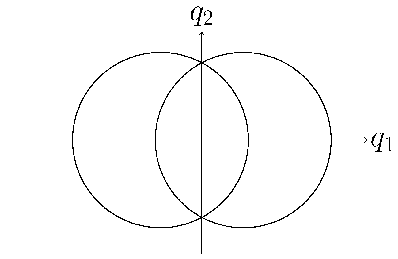
Figure 1. Symmetries of A ( x / 2 , 0 ) A ( x / 2 , 0 ) .
Symmetry 12 01265 g001
Figure 2. Third-order structure function S 3 ( x ) as a function of x in double-logarithmic representation for the kernel (17). The straight line for small x indicates a scaling behavior x 3 and the straight line for large x indicates a linear behavior x .
Symmetry 12 01265 g002