Article

A Generalization of Binomial Exponential-2 Distribution: Copula, Properties and Applications

1
Department of Mathematics and Statistics-College of Science, Imam Mohammad ibn Saud, Islamic University (IMSIU), Riyadh 11432, Saudi Arabia
2
Department of Mathematics and Informatics, Yuriy Fedkovych Chernivtsi National University, 28 Universytetska Street, 58012 Chernivtsi, Ukraine
*
Author to whom correspondence should be addressed.
Symmetry 2020, 12(8), 1338; https://doi.org/10.3390/sym12081338
Submission received: 26 July 2020 / Revised: 4 August 2020 / Accepted: 7 August 2020 / Published: 10 August 2020
(This article belongs to the Section Mathematics)

Abstract

:
In this paper, we propose a new three-parameter lifetime distribution for modeling symmetric real-life data sets. A simple-type Copula-based construction is presented to derive many bivariate- and multivariate-type distributions. The failure rate function of the new model can be “monotonically asymmetric increasing”, “increasing-constant”, “monotonically asymmetric decreasing” and “upside-down-constant” shaped. We investigate some of mathematical symmetric/asymmetric properties such as the ordinary moments, moment generating function, conditional moment, residual life and reversed residual functions. Bonferroni and Lorenz curves and mean deviations are discussed. The maximum likelihood method is used to estimate the model parameters. Finally, we illustrate the importance of the new model by the study of real data applications to show the flexibility and potentiality of the new model. The kernel density estimation and box plots are used for exploring the symmetry of the used data.

1. Introduction

The monotonicity asymmetric failure (hazard) rate function (HRF) of a certain lifetime probabilistic distribution has an important role in modeling real lifetime data. Distributions with the “monotonicity increasing” failure rate (MIFR) function have useful real applications in “pricing” and “supply” chain contracting problems. The MIFR property is a well-known and useful concept in “dynamic programming”, “reliability theory” and other areas of applied probability and statistics (see [1,2]). The paper [3] introduced a new two-parameter lifetime model with MIFR named the binomial-exponential-2 (BE2) model, which is constructed as a model of a random sum (RSm) of independent exponential random variables (RVs) when the sample size has a “zero truncated binomial” distribution. The BE2 distribution can be used as an alternative to the Weibull (W), gamma (Gam), exponentiated exponential (EE), and weighted exponential (WhE) distributions in real life applications.
The survival function (SF) of the binomial exponential-2 (BE2) distribution is given by
G ¯ B E 2 ( y ) = ( 1 + θ α y 2 θ ) e α y | y > 0 ( 0 θ 1 ) ,
where α > 0 is a scale parameter, G B E 2 ( y ) = 1 G ¯ B E 2 ( y ) is the cumulative distribution function (CDF) of the BE2 model and θ is a shape parameter. It is easy to show that the SF in (1) is increasing in 0 θ 1 where e α y G ¯ B E 2 ( y ) ( α y + 1 ) e α y 1 (see [2]). The probability density function (PDF) corresponding to (1) is
g B E 2 ( y ) = [ 1 + θ 2 θ ( α y 1 ) ] α e α y ,
which can be expressed as
g B E 2 ( y ) = α 2 θ [ 2 ( 1 θ ) + α y   θ ] e α y .
Since 2 y 2 is negative, the l o g [ g B E 2 ( y ) ] is “concave” for all α and 0 θ 1. As a result, g B E 2 ( y ) is “log-concave” and “unimodal”. Additionally, the PDF (2) can be written as
g B E 2 ( y ) = π ( θ ) α e α y + π ¯ ( θ ) α 2 y e α y ,
where
π ( θ ) = 2 2 θ ( 1 θ )   and   π ¯ ( θ ) = 1 π ( θ ) . π ( θ ) = 2 2 θ ( 1 θ )   and   π ¯ ( θ ) = 1 π ( θ ) .
The BE2 model is a mixture of the standard exponential (with parameter α ) model and standard gamma model (with shape parameter 2 and scale parameter α ); when θ = 0 , we get the standard exponential model, and when θ = 1 , the BE2 model reduces to the Gam model. In the last few decades, many new G families of continuous distributions have been developed. One of the most famous ones is called the new type II half-logistic (TIIHL-G) family (see [4]). According to [4], the CDF of the TIIHL-G family of distributions is given by
F λ , Ψ _ ( y ) = 2 G Ψ _ ( y ) λ 1 + G Ψ _ ( y ) λ ,
where G Ψ _ ( y ) is the baseline CDF depending on a parameter vector Ψ _ and λ > 0 is an additional shape parameter. For each baseline G Ψ _ ( y ) , we can generate a new TIIHL model using (4). The corresponding PDF to (4) is given by
f λ , Ψ _ ( y ) = 2 λ g Ψ _ ( y ) G Ψ _ ( y ) λ 1 [ 1 + G Ψ _ ( y ) λ ] 2 ,
where g Ψ _ ( y ) = d G Ψ _ ( y ) / d x is the baseline PDF. Equation (5) will be most tractable when G Ψ _ ( y ) and g Ψ _ ( y ) have simple expressions. The survival function, the failure (hazard) rate function and the quantile function are F ¯ λ , Ψ _ ( y ) = 1 G Ψ _ ( y ) λ 1 + G Ψ _ ( y ) λ , h λ , Ψ _ ( y ) = 2 λ g Ψ _ ( y ) G Ψ _ ( y ) λ 1 1 G Ψ _ ( y ) 2 λ , and Q ( u ) = G 1 u 2 u λ . Equations (4) and (5) are used for generating the new model.

2. The New Model and Its Motivation

In this section, we introduce the three-parameter type II half-logistic binomial exponential 2 (TIIHLBE2) distribution. Substituting from (1) into (4), the CDF of the TIIHLBE2 (or expanded BE2 “EBE” for short) model can be expressed as
F λ , α , θ ( y ) = 2 [ 1 ( 1 + θ α y 2 θ ) e α y ] λ 1 + [ 1 ( 1 + θ α y 2 θ ) e α y ] λ ,
The corresponding PDF is given by
f λ , α , θ ( y ) = 2 λ α e α y ( 1 + ( α y 1 ) θ 2 θ ) [ 1 ( 1 + θ α y 2 θ ) e α y ] λ 1 { 1 + [ 1 ( 1 + θ α y 2 θ ) e α y ] λ } 2 .
Here and henceforth, an RV Y having PDF (7) is denoted by Y EBE ( λ , α , θ ) . For the EBE distribution, the HRF can be derived as
h λ , α , θ ( y ) = 2 λ α e α y ( 1 + ( α y 1 ) θ 2 θ ) [ 1 ( 1 + θ α y 2 θ ) e α y ] { 1 + [ 1 ( 1 + θ α y 2 θ ) e α y ] λ } .
Figure 1 presents some plots of the PDF of the EBE model for some different values of the parameters λ , α and θ . We note that the new PDF can be “right skewed” with different shapes of “skewness” and “kurtosis”.
Figure 2 gives the plots of the HRF of the EBE distribution. We note that the new HRF can be “increasing”, “increasing-constant”, “decreasing” and “upside-down-constant” shaped. Thus, the new model may be useful in modeling different shapes of real data.

3. Copula under the EBE Model

3.1. Bivariate EBE (BivEBE) Type via Renyi’s Entropy

Following [5], the joint CDF (JCDF) of the “Renyi’s entropy Copula” can be expressed as
C ( 𝓊 , v ) = y 2 𝓊 + y 1 v y 1 y 2 ; then, the associated BivEBE will be 𝓗 ( t 1 , t 2 ) = 𝓗 ( F V _ 1 ( y 1 ) , F V _ 2 ( y 2 ) ) where V _ 1 and V _ 2 are the parameter vectors for F V _ 1 ( y 1 ) and F V _ 2 ( y 2 ) , respectively.

3.2. BivEBE Type Using “Farlie-Gumbel-Morgenstern” (FGM) Copula

Consider the JCDF of the FGM family, where 𝓗 Δ ( 𝓊 , v ) = u v ( 1 + Δ 𝓊 ¯ v ¯ ) | Δ [ 1 , 1 ] . The marginal functions are 𝓊 = F 1 ( y 1 ) [ 0 , 1 ] and v = F 2 ( y 2 ) [ 0 , 1 ] . The unknown parameter Δ is a dependence parameter, and for every 𝓊 , v [ 0 , 1 ] , 𝓗 Δ ( 𝓊 , 0 ) = C Δ ( 0 , v ) = 0 , which is the “grounded minimum” property, and 𝓗 Δ ( 𝓊 , 1 ) = u and 𝓗 Δ ( 1 , v ) = v , which is “grounded maximum” property. 𝓊 ¯ = 𝓊 ¯ V _ 1 = 1 F V _ 1 ( y 1 )   and v ¯ = v ¯ V _ 2 = 1 F V _ 2 ( y 2 ) are then set.
Then, F ( y 1 , y 2 ) = 𝓗 ( F V _ 1 ( y 1 ) , F V _ 2 ( y 2 ) .   The joint PDF can be derived from
h Δ ( 𝓊 , v ) = Δ 𝓊 v + 1 | ( 𝓊 = 1 2 𝓊   and   v = 1 2 v )
or from
f ( y 1 , y 2 ) = h ( F V _ 1 ( y 1 ) , F V _ 2 ( y 2 ) ) f V _ 1 ( y 1 ) f V _ 2 ( y 2 ) .
For more details, see [6,7,8,9,10,11,12].

3.3. BivEBE Type via “Modified FGM” (MFGM) Copula

The modified JCDF of the bivariate FGM copula can be expressed as
𝓗 Δ ( 𝓊 , w ) = 𝓊 v + Δ O ( 𝓊 ) ˜ φ ( w ) ˜ ,
where O ( 𝓊 ) ˜ = 𝓊 O ( 𝓊 ) ¯ and φ ( w ) ˜ = w φ ( w ) ˜ , where O ( 𝓊 ) and φ ( w ) are two absolutely continuous functions on ( 0 , 1 ) where O ( 0 ) = O ( 1 ) = φ ( 0 ) = φ ( 1 ) = 0. Let
α = i n f { 𝓊 O ( 𝓊 ) ˜ : C 1 } < 0 , β = s u p { 𝓊 O ( 𝓊 ) ˜ : C 1 } < 0 , ξ = i n f { w φ ( w ) ˜ : C 2 } > 0 , η = s u p { w φ ( w ) ˜ : C 2 } > 0.
Then,
m i n ( β α , η ξ ) 1 ,
where
O ( 𝓊 ) + 𝓊 𝓊 O ( 𝓊 ) = 𝓊 O ( 𝓊 ) ˜ , C 1 = { 𝓊 ( 0 , 1 ) : 𝓊 O ( 𝓊 ) ˜   exists } ,
and
C 2 = { w ( 0 , 1 ) : w φ ( w ) ˜   exists } .

3.3.1. BivEBE-FGM (Type-I) Model

The BivEBE-FGM (Type-I) model can be derived directly using
𝓗 Δ ( 𝓊 , w ) = Δ O ( 𝓊 ) ˜ φ ( w ) ˜ + 𝓊 v ,

3.3.2. BivEBE-FGM (Type-II) Model

Consider O ( 𝓊 ) and φ ( w ) that satisfy all the conditions stated earlier where
O ( 𝓊 ) | ( Δ 1 > 0 ) = 𝓊 Δ 1 ( 1 𝓊 ) 1 Δ 1   and   φ ( w ) | ( Δ 2 > 0 ) = v Δ 2 ( 1 w ) 1 Δ 2 .
The corresponding BivEBE-FGM (Type-II) copula can be derived from
C Δ , Δ 1 , Δ 2 ( 𝓊 , w ) = u w [ 1 + Δ 𝓊 Δ 1 w Δ 2 ( 1 𝓊 ) 1 Δ 1 ( 1 w ) 1 Δ 2 ] .

3.3.3. BivEBE-FGM (Type-III) Model

Consider O ( 𝓊 ) and φ ( w ) that satisfy all the conditions stated earlier where
O ( 𝓊 ) = 𝓊 [ l o g ( 1 + 𝓊 ¯ ) ]   and   φ ( w ) = w [ l o g ( 1 + w ¯ ) ] .
In this case, one can also derive a closed form expression for the associated CDF of the BivEBE-FGM (Type-III).

3.3.4. BivEBE-FGM (Type-IV) Model

The JCDF of the BivEBE-FGM (Type-IV) model can be derived from
𝓗 ( 𝓊 , w ) = 𝓊 F 1 ( w ) + w F 1 ( 𝓊 ) F 1 ( 𝓊 ) F 1 ( w ) .

3.4. BivEBE Type via Clayton Copula

The Clayton Copula can be considered as
𝓗 ( 𝓊 1 , 𝓊 2 ) = ( 𝓊 1 Δ + 𝓊 2 Δ 1 ) 1 Δ | Δ [ 0 , ] .
Let T EBE ( V _ 1 ) and W EBE ( V _ 2 ) . Set 𝓊 1 = 𝓊 ( t ) = F V _ 1 ( t ) | V _ 1 > 0 and 𝓊 2 = 𝓊 ( w ) = F V _ 1 ( w ) | V _ 2 > 0 . Then, the BivEBE-type distribution can be derived from F ( t , w ) = 𝓗 ( F V _ 1 ( t ) , F V _ 2 ( w ) ) . A straightforward n -dimensional extension from the above will be 𝓗 ( 𝓊 i ) = [ 1 n + i = 1 n 𝓊 i Δ ] 1 Δ . Many other useful details can be found in [13,14,15,16,17,18,19,20,21,22].

4. Properties

4.1. Expansions and Quantile Function (QF)

Consider the series representation
( ω 1 ω 2 + 1 ) ω 3 = i = 0 ( ω 1 ω 2 ) i ( ω 3 + i 1 i ) | ( | ω 1 ω 2 | 1   and   ω 3 0 ) ;
expanding { 1 + [ 1 ( 1 + θ α y 2 θ ) e α y ] λ } 2 , we can write (7) as
f ( y ) = 2 λ α i = 0 ( 1 ) i   ( i + 1 ) e α y ( 1 + ( α y 1 ) θ 2 θ ) [ 1 ( 1 + θ α y 2 θ ) e α y ] λ ( i + 1 ) 1 .
Then, consider the power series expansion
( 1 ω 1 ω 2 ) ω 3 1 = j = 0 ( ω 1 ω 2 ) j ( ω 3 1 j ) | ( | ω 1 ω 2 | 1   and   ω 3 0 ) ;
using (11) in Equation (10), and after some algebra, the PDF of EBE can be written as
f ( y ) = 2 λ α i , j = 0 ( 1 ) i ( i + 1 ) ( λ ( i + 1 ) 1 j ) ( 1 + ( α y 1 ) θ 2 θ ) ( 1 + θ α y 2 θ ) j e α ( 1 + j ) y ,
Then, we have
( 1 + θ α y 2 θ ) j = κ = 0 ( j κ ) ( θ α 2 θ ) κ y κ   ;  
therefore, the PDF of the EBE model becomes
f ( y ) = κ = 0 C κ   Π θ , α j , κ ( y ) ,
where
C κ = 2 λ i , j = 0 α 1 + κ   ( 1 ) i ( i + 1 ) ( λ ( i + 1 ) 1 j ) ( j κ ) θ κ ( 2 θ ) 1 + κ ,
and
Π θ , α j , κ ( y ) = [ 2 ( 1 θ ) y κ + θ α y κ + 1 ] e α ( 1 + j ) y .
The QF of the EBE model is given by the real solution of the following equation:
( 1 + θ α y q 2 θ ) e α y p + ( q 2 q ) 1 λ = 1 ,
where the above equation has no closed form solution in y q , so we have to use a numerical technique.

4.2. Moments

Theorem 1.
If Y EBE ( λ , α , θ ) , then the r t h moment of Y is given by
μ r ( y ) = κ = 0 C κ r Γ ( r + κ + 1 ) ,
where
C κ r = C κ 2 α ( 1 + j ) ( 1 θ ) + θ α ( r + κ + 1 ) [ α ( 1 + j ) ] r + κ + 2 .
Proof. 
Let Y be an RV following the EBE distribution. The r t h ordinary moment can be obtained using the well-known formula
μ r ( y ) = 0 f ( y ) y r d y = κ = 0 C κ   0 y r Π θ , α j , κ ( y ) d y ,
then
μ r ( y ) = κ = 0 C κ   0 [ 2 ( 1 θ ) y r + κ + θ α y r + κ + 1 ] e α ( 1 + j ) y d y .
Setting x = α ( 1 + j ) y , after some algebra, we obtain
μ r ( y ) = κ = 0 j C κ r Γ ( r + κ + 1 ) .
If we set r = 1 , we obtain the mean of the EBE distribution. Variance, skewness and kurtosis measures can be easily derived from the well-known relationships. Three-dimensional plots of the skewness and kurtosis of the EBE model are presented in Figure 3 and Figure 4. □
These plots indicate that both measures depend very much on the shape parameter θ . The first four moments and the skewness and kurtosis of the EBE distribution for different values of parameters are represented in Table 1.
Theorem 2.
The moment generating function M Y ( τ ) of the EBE is given by
M Y ( τ ) = κ = 0 C κ ( r , τ ) Γ ( κ + 1 ) ,
where
C κ ( r , τ ) = C κ 2 ( 1 θ ) ( α ( 1 + j ) τ ) + θ α ( κ + 1 ) [ α ( 1 + j ) ] κ + 2 .
Proof. 
Starting with
M Y ( τ ) = E ( e τ Y ) = 0 e τ Y f ( y ) d y ,
then
M Y ( τ ) = κ = 0 C κ   0 [ 2 ( 1 θ ) y κ + 1 + θ α y κ + 2 ] e [ α ( 1 + j ) τ ] y d y ,
finally, we get
M Y ( τ ) = κ = 0 C κ ( r , τ ) Γ ( κ + 1 ) .
In the same way, the characteristic function of the EBE distribution becomes
ϕ Y ( τ ) = M Y ( i τ )
where i = 1 is the unit imaginary number. □

4.3. Incomplete Moments

The s t h lower and upper incomplete moments of Y are defined by
υ s , Y ( τ ) = E ( Y s | ( Y < τ ) ) = 0 τ y s f ( y ) d y ,
and
v s , Y ( τ ) = E ( Y s | ( Y > τ ) ) = τ y s f ( y ) d y ,
respectively, for any real s > 0. The s t h lower incomplete moment of the EBE distribution is
v s , Y ( τ ) = 0 τ y s f ( y ) d y = κ = 0 C κ   0 τ [ 2 ( 1 θ ) y s + κ + θ α y s + κ + 1 ] e α ( 1 + j ) y d y ,
then
v s , Y ( τ ) = κ = 0 C κ [ c ( s , j ) ( 1 ) γ ( s + κ + 1 , α ( 1 + j ) τ ) + c ( s , j ) ( 2 ) γ ( s + κ + 2 , α ( 1 + j ) τ ) ] ,
where c ( Δ , j ) ( 1 ) = 2 ( 1 θ ) 1 [ α ( 1 + j ) ] Δ + κ + 1 , c ( Δ , j ) ( 2 ) = θ α 1 [ α ( 1 + j ) ] Δ + κ + 2 and γ ( s , τ ) = 0 τ y s 1 e y d y is the lower incomplete gamma function. Similarly, the s t h upper incomplete moment of the EBE distribution is
η s ( τ ) = τ y s f ( y ) d y = κ = 0 C κ   τ [ 2 ( 1 θ ) y s + κ + θ α y s + κ + 1 ] e α ( 1 + j ) y d y ,
then
η s ( τ ) = κ = 0 C κ [ c ( s , j ) ( 1 ) ζ ( s + κ + 1 , α ( 1 + j ) τ ) + c ( s , j ) ( 2 ) ζ ( s + κ + 2 , α ( 1 + j ) τ ) ] ,
where
ζ ( s , τ ) = τ e y y s 1 d y ,
is the upper incomplete gamma function.

4.4. Mean Deviation and Bonferroni and Lorenz Curve

The mean deviations about the mean μ = E ( Y ) and the mean deviations about the median M can be written as
δ 1 ( y ) = 2 [ μ F ( μ ) ϖ ( μ ) ] = 0 f ( y ) | y μ | d y ,
and
δ 2 ( y ) = μ 2 ϖ ( M ) = 0 f ( y ) | y M | d y ,
respectively, where
ϖ ( d ) = 0 d y   f ( y ) d y = κ = 0 C κ [ c ( 1 , j ) ( 1 ) γ ( κ + 2 , α ( 1 + j ) d ) + c ( 1 , j ) ( 2 ) γ ( κ + 3 , α ( 1 + j ) d ) ] .
The Lorenz curve for a positive RV Y is defined as
L ( p ) = 1 μ 0 h y ( f ) d y = ϖ ( h ) μ = 1 μ κ = 0 C κ [ c ( 1 , j ) ( 1 ) γ ( κ + 2 , α ( 1 + j ) h ) + c ( 1 , j ) ( 2 ) γ ( κ + 3 , α ( 1 + j ) h ) ] ,
where h = G 1 ( p ) . Additionally, the Bonferroni curve is defined by
B ( p ) = 1 μ p 0 h y ( f ) d y = ϖ ( h ) μ p = 1 μ p κ = 0 C κ [ c ( 1 , j ) ( 1 ) γ ( κ + 2 , α ( 1 + j ) h ) + c ( 1 , j ) ( 2 ) γ ( κ + 3 , α ( 1 + j ) h ) ] ,

4.5. Residual Life and Reversed Residual Life Functions

The r τ h moment of the residual life via the general formula is given by
μ r , Y ( τ ) = E ( ( Y τ ) r | ( Y > τ ) ) = 1 F ¯ ( τ ) τ f ( y ) ( y τ ) r d y | ( r 1 ) = 1 F ¯ ( τ ) κ = 0 C κ h = 0 r ( r h ) ( 1 ) r h τ r i τ [ 2 ( 1 θ ) y r + κ + θ α y r + κ + 1 ] e α ( 1 + j ) y d y ,
then
μ r , Y ( τ ) = 1 F ¯ ( τ ) κ = 0 C κ h = 0 r ( 1 ) r h ( r h ) τ r i [ c ( r , j ) ( 1 ) ζ ( r + κ + 1 , α ( 1 + j ) τ ) + c ( r , j ) ( 2 ) ζ ( r + κ + 2 , α ( 1 + j ) τ ) ] .
The mean residual life (MRL) of the EBE distribution is given by
μ 1 , Y ( τ ) = 1 F ¯ ( τ ) κ = 0 C κ [ c ( 1 , j ) ( 1 ) ζ ( κ + 2 , α ( 1 + j ) τ ) + c ( 1 , j ) ( 2 ) ζ ( κ + 3 , α ( 1 + j ) τ ) ] τ
The r t h order moment of the reversed residual life can be obtained by the well-known formula
m r , Y ( τ ) = E ( ( τ y ) r | ( Y τ ) ) = 1 F ( τ ) 0 τ f ( y ) ( τ y ) r d y | ( r 1 ) .
Applying the binomial expansion of ( τ y ) r and substituting f λ , α , θ ( y ) given by (7) into the above formula gives
m r , Y ( τ ) = 1 F ( τ ) h = 0 r κ = 0 C κ ( r h ) ( 1 ) r h τ r i 0 τ [ 2 ( 1 θ ) y r + κ + θ α y r + κ + 1 ] e α ( 1 + j ) y d y ,
then
m r , Y ( τ ) = 1 F ( τ ) κ = 0 C κ h = 0 r ( r h ) ( 1 ) r h τ r i × [ c ( r , j ) ( 1 ) γ ( r + κ + 1 , α ( 1 + j ) τ ) + c ( r , j ) ( 2 ) γ ( r + κ + 2 , α ( 1 + j ) τ ) ] ,
where
γ ( s , p ) = 0 p w s 1 e w d w ,
is the lower incomplete gamma function. The mean waiting time of the EBE distribution is given by
m 1 ( τ ) = τ 1 F ( τ ) κ = 0 C κ [ c ( 1 , j ) ( 1 ) γ ( κ + 2 , α ( 1 + j ) τ ) + c ( 1 , j ) ( 1 ) γ ( κ + 3 , α ( 1 + j ) τ ) ] .
Using m 1 , Y ( τ ) and m 2 , Y ( τ ) , one can obtain the “variance” and the “coefficient of variation” of the reversed residual life of the EBE distribution.

5. Estimation and Inference

Let Y 1 , Y 2 , , Y n be a random sample of size n from EBE ( ψ _ ) . The log likelihood function for the vector of parameters λ , α and θ can be written as
l o g L = n l o g ( 2 λ ) + n l o g α n l o g ( 2 2 θ ) α i = 1 n y i + ( λ 1 ) i = 1 n l o g ( 1 m i s i ) 2 i = 1 n l o g [ 1 + ( 1 m i s i ) λ ] ,
where m i = 1 + θ α y i 2 θ and s i = e α y i . The associated score function is given by
U n ( ψ _ ) = [ l o g L λ , l o g L α , l o g L θ ] T .
The l o g L in (18) can be maximized by solving the nonlinear likelihood equations obtained by differentiating (18). The components of the score vector are given by
U λ = l o g   L λ = n λ + i = 1 n l o g ( 1 m i s i ) 2 i = 1 n ( 1 m i s i ) λ l o g ( 1 m i s i ) 1 + ( 1 m i s i ) λ , U α = l o g   L α = n α i = 1 n y i + ( λ 1 ) i = 1 n s i [ α m i + θ y i 2 θ ] 1 m i s i 2 λ i = 1 n s i [ 1 m i s i ] λ 1 ( α m i + θ y i 2 θ ) 1 + ( 1 m i s i ) λ
U α = l o g   L α = n α i = 1 n y i + ( λ 1 ) i = 1 n s i [ α m i + θ y i 2 θ ] 1 m i s i 2 λ i = 1 n s i [ 1 m i s i ] λ 1 ( α m i + θ y i 2 θ ) 1 + ( 1 m i s i ) λ
and
U θ = l o g   L θ = n 1 θ 2 ( λ 1 ) i = 1 n α ( 2 θ ) 2 y s i 1 m i s i + ( λ 1 ) i = 1 n α l o g ( y i ) y i β e α   y i β 1 e α   y i β 4 λ i = 1 n α y s i ( 2 θ ) 2 ( 1 m i s i ) λ 1 1 + ( 1 m i s i ) λ

6. Simulation

The “inverse transform algorithm” is used to generate random data from the EBE distribution. We generated samples of sizes n = 50 , 100 , 200 , 500 and 1000 , and the simulations were repeated N = 1000 times from the EBE model for some parameter values. Table 2 and Table 3 give the mean square errors (MSEs) and the biases, respectively. The average values of estimates (AVs), estimated average length (EAL) and the coverage probability (CP) are listed in Table 4, Table 5 and Table 6, respectively. From Table 2, we note that the AVs of estimates approach the initial values as n , the MSEs for each parameter decrease to zero as n , and the coverage lengths for each parameter decrease to zero as n . From Table 3, we note that the biases for each parameter are generally positive and decrease to zero as n , and the coverage probabilities for each parameter approach the nominal level as n .

7. Modeling Stress-Rupture Life of Kevlar 49/Epoxy Strands Data

In this section, we illustrate the performance of the EBE distribution as compared to some alternative distributions using a real data application. The goodness-of-fit (GOF) statistics for this distribution are compared with other competitive distributions, and the maximum likelihood estimations (MLEs) of the distribution parameters are determined numerically. We compare the fits of the EBE distribution with the Burr type X (Burr X) distribution, Burr type XII (Burr XII) distribution, beta log logistic Weibull distribution (BLLW), beta Weibull log logistic (BWLL) and beta log logistic, beta linear failure rate geometric (BLFRG), exponentiated linear failure rate geometric (ELFRG), beta Rayleigh (BR), and beta Weibull geometric distributions (BWG) (see [23]). In order to compare the distributions, we consider the measures of GOF including the Akaike Information Criterion (C [ 1 ] ), Bayesian Information Criterion (C [ 2 ] ), Consistent Akaike Information Criterion (C [ 4 ] ) and Hannan–Quinn Information Criterion (C [ 3 ] ) statistics.
The following real data set represents the stress-rupture life of Kevlar 49/epoxy strands that are subjected to constant sustained pressure at the 90% stress level until all have failed that were provided by [24], given as 0.01, 0.08, 0.09, 0.09, 0.10, 0.02, 0.02, 0.03, 0.03, 0.04, 0.05, 0.43, 0.52, 0.54, 0.56, 0.60, 0.60, 1.00, 0.06, 1.34, 0.10, 1.45, 1.50, 1.51, 0.63, 0.72,0.99, 1.52, 1.53, 1.54, 1.54, 1.55, 1.58, 4.20, 4.69, 7.89, 0.07, 0.07, 0.36, 0.38, 0.40, 0.65, 0.67, 0.68, 0.79, 0.80, 0.80, 0.83, 0.72, 0.42, 0.12, 0.13, 0.18, 0.19, 0.20, 0.23, 0.24, 1.01, 1.02, 1.03, 0.72, 0.73, 0.79, 0.85, 0.90, 0.92, 0.95, 1.05, 0.11, 0.24, 0.29, 0.34, 0.35, 1.10, 1.10, 1.11, 1.15, 1.18, 1.20, 1.29, 1.31, 0.11, 0.01, 0.02, 1.40, 1.43 and 1.33. Table 7 gives the MLE for all the models corresponds to the failure times data set. Table 8 shows the statistics for the failure times of the Kevlar data set. Figure 5 gives the kernel density estimation and box plot for exploring the symmetry of the stress-rupture life data. Figure 6 provides the fitted PDF in the left panel and fitted CDF in the right panel.
Based on Table 8, it is clear that the EBE distribution provides the best fit to these data, with −2logL = 143.3996, C [ 1 ] = 149.41, C [ 4 ] = 149.6887, C [ 2 ] = 152.3784 and C [ 3 ] = 152.3784. Thus, it is concluded that this model can be a better model than other competitive lifetime models for explaining the data set. Based on Figure 6, we note that the EBE distribution gives adequate fits. Many symmetric and near symmetric real-life data sets can be modeled using the new EBE model and found in [25,26,27,28,29,30,31,32,33,34,35,36]. For other right heavy tailed real data sets see [37,38,39,40,41,42,43,44,45]. As a future work we will consider “bivariate” and “multivariate” extensions of the EBE distribution. In particular with the “copula-based construction” method, “trivariate reduction” etc.

8. Conclusions

A new three-parameter lifetime distribution is proposed and studied. A simple-type Copula-based construction is presented to derive many bivariate- and multivariate-type distributions. We investigated some of mathematical properties such as the ordinary moments, moment generating function and conditional moment. Bonferroni and Lorenz curves and mean deviations are discussed. Residual life and reversed residual functions are also obtained. Some bivariate- and multivariate-type extensions are proposed. The maximum likelihood method is used to estimate the model parameters. Finally, we illustrate the importance of the new model by studying real data applications to show the flexibility and potentiality of the new model.

Author Contributions

All authors contributed equally to this work. All authors have read and agreed to the published version of the manuscript.

Funding

This research received no external funding.

Acknowledgments

The authors acknowledge the College of Science at Al Imam Mohammad Ibn Saud Islamic University, Saudi Arabia, for supporting this project.

Conflicts of Interest

The authors declare no conflict of interest regarding the publication of this paper.

References

  1. Shaked, M.; Shanthikumar, J. Stochastic Orders; Springer: NewYork, NY, USA, 2007. [Google Scholar]
  2. Bakouch, H.S.; Jazi, M.A.; Nadarajah, S.; Dolati, A.; Roozegar, R. A lifetime model with increasing failure rate. Appl. Math. Model. 2014, 38, 5392–5406. [Google Scholar] [CrossRef]
  3. Asgharzadeh, A.; Bakouch, H.S.; Habibi, M. A generalized binomial exponential 2 distribution: Modeling and applications to hydrologic events. J. Appl. Stat. 2016, 44, 2368–2387. [Google Scholar] [CrossRef]
  4. Soliman, A.H.; Elgarhy, M.A.E.; Shakil, M. Type II Half Logistic Family of Distributions with Applications. Pak. J. Stat. Oper. Res. 2017, 13, 245. [Google Scholar] [CrossRef] [Green Version]
  5. Pougaza, D.B.; Mohammad-Djafari, A. Maximum entropies copulas. In AIP Conference Proceedings; American Institute of Physics: College Park, MD, USA, 2011; Volume 1305, pp. 329–336. [Google Scholar]
  6. Morgenstern, D. Einfache beispiele zweidimensionaler verteilungen. Mitteilingsblatt Math. Stat. 1956, 8, 234–235. [Google Scholar]
  7. Farlie, D.J.G. The performance of some correlation coefficients for a general bivariate distribution. Biometrika 1960, 47, 307–323. [Google Scholar] [CrossRef]
  8. Johnson, N.L.; Kotz, S. On some generalized Farlie- Gumbel- Morgenstern distributions. Commun. Stat. Theory 1975, 4, 415–427. [Google Scholar] [CrossRef]
  9. Johnson, N.L.; Kotz, S. On some generalized Farlie-Gumbel-Morgenstern distributions-II: Regression, correlation and further generalizations. Commun. Stat. Theory 1977, 6, 485–496. [Google Scholar] [CrossRef]
  10. Gumbel, E.J. Bivariate logistic distributions. J. Am. Stat. Assoc. 1961, 56, 335–349. [Google Scholar] [CrossRef]
  11. Gumbel, E.J. Bivariate exponential distributions. J. Am. Stat. Assoc. 1960, 55, 698–707. [Google Scholar] [CrossRef]
  12. Gupta, R.C.; Gupta, R.D. Proportional reversed hazard rate model and its applications. J. Stat. Plan Inference 2007, 137, 3525–3536. [Google Scholar] [CrossRef]
  13. Alizadeh, M.; Ghosh, I.; Yousof, H.M.; Rasekhi, M.; Hamedani, G.G. The generalized odd generalized exponential family of distributions: Properties, characterizations and applications. J. Data Sci. 2017, 15, 443–466. [Google Scholar]
  14. Alizadeh, M.; Rasekhi, M.; Yousof, H.M.; Hamedani, G.G. The transmuted Weibull G family of distributions. Hacet. J. Math. Stat. 2018, 47, 1–20. [Google Scholar] [CrossRef]
  15. Al-Babtain, A.A.; Elbatal, I.; Yousof, H.M. A new flexible three-parameter model: Properties, Clayton Copula, and modeling real data. Symmetry 2020, 12, 440. [Google Scholar] [CrossRef] [Green Version]
  16. Al-Babtain, A.A.; Elbatal, I.; Yousof, H.M. A new three parameter Fréchet model with mathematical properties and applications. J. Taibah Univ. Sci. 2020, 14, 265–278. [Google Scholar] [CrossRef] [Green Version]
  17. Mansour, M.; Yousof, H.M.; Shehata, W.A.; Ibrahim, M. A new two parameter Burr XII distribution: Properties, Copula, different estimation methods and modeling acute bone cancer data. J. Nonlinear Sci. Appl. 2020, 13, 223–238. [Google Scholar] [CrossRef] [Green Version]
  18. Yadav, A.S.; Goual, H.; Alotaibi, R.M.; Ali, M.M.; Yousof, H.M. Validation of the Topp-Leone-Lomax model via a modified Nikulin-Rao-Robson goodness-of-fit test with different methods of estimation. Symmetry 2020, 12, 57. [Google Scholar] [CrossRef] [Green Version]
  19. Yousof, H.M.; Butt, N.S.; Alotaibi, R.; Rezk, H.; Alomani, A.G.; Ibrahim, M. A new compound Fréchet distribution for modeling breaking stress and strengths data. Pak. J. Stat. Oper. Res. 2019, 15, 1017–1035. [Google Scholar] [CrossRef]
  20. Yousof, H.M.; Mansoor, M.M.; Alizadeh, M.; Afify, A.Z.; Ghosh, I.; Afify, A.Z. The Weibull-G Poisson family for analyzing lifetime data. Pak. J. Stat. Oper. Res. 2020, 16, 131–148. [Google Scholar] [CrossRef]
  21. Ibrahim, M.; Yadaw, A.S.; Yousof, A.S.; Goual, H.; Hamedani, G.G. A new extension of Lindley distribution: Modified validation test, characterizations and different methods of estimation. Commun. Stat. Appl. Methods 2019, 26, 473–495. [Google Scholar] [CrossRef]
  22. Goual, H.; Yousof, H.M.; Ali, M.M. Validation of the odd Lindley exponentiated exponential by a modified goodness of fit test with applications to censored and complete data. Pak. J. Stat. Oper. Res. 2019, 15, 745–771. [Google Scholar] [CrossRef]
  23. Bidram, H.; Behboodian, J.; Towhidi, M. The Beta Weibull-Geometric Distribution. J. Stat. Comput. Simul. 2013, 83, 52–67. [Google Scholar] [CrossRef]
  24. Cooray, K.; Ananda, M. A Generalization of the Half-Normal Distribution with Application to Lifetime Data. Commun. Stat. Theory Methods 2008, 37, 1323–1337. [Google Scholar] [CrossRef]
  25. Korkmaz, M.Ç.; Yousof, H.M.; Ali, M.M. Some theoretical and computational aspects of the odd Lindley Fréchet distribution. İstatistikçiler Dergisi: İstatistik ve Aktüerya 2017, 10, 129–140. [Google Scholar]
  26. Korkmaz, M.Ç.; Yousof, H.M. The one-parameter odd Lindley exponential model: Mathematical properties and applications. Stoch. Qual. Control 2017, 32, 25–35. [Google Scholar] [CrossRef]
  27. Korkmaz, M.Ç.; Alizadeh, M.; Yousof, H.M.; Butt, N.S. The generalized odd Weibull generated family of distributions: Statistical properties and applications. Pak. J. Stat. Oper. Res. 2018, 14, 541–556. [Google Scholar] [CrossRef] [Green Version]
  28. Korkmaz, M.Ç.; Yousof, H.M.; Rasekhi, M.; Hamedani, G.G. The Odd Lindley Burr XII Model: Bayesian Analysis, Classical Inference and Characterizations. J. Data Sci. 2018, 16, 327–353. [Google Scholar]
  29. Korkmaz, M.Ç.; Yousof, H.M.; Hamedani, G.G. The exponential Lindley odd log-logistic-G family: Properties, characterizations and applications. J. Stat. Theory Appl. 2018, 17, 554–571. [Google Scholar] [CrossRef] [Green Version]
  30. Hamedani, G.G.; Yousof, M.H.; Rasekhi, M.; Alizadeh, M.; Najibi, S.M. Type I general exponential class of distributions. Pak. J. Stat. Oper. Res. 2018, 14, 39–55. [Google Scholar] [CrossRef] [Green Version]
  31. Hamedani, G.G.; Altun, E.; Korkmaz, M.Ç.; Yousof, H.M.; Butt, N.S. A new extended G family of continuous distributions with mathematical properties, characterizations and regression modeling. Pak. J. Stat. Oper. Res. 2018, 14, 737–758. [Google Scholar] [CrossRef] [Green Version]
  32. Yousof, H.M.; Korkmaz, Ç.M.; Hamedani, G.G. The odd Lindley Nadarajah-Haghighi distribution. J. Math. Comput. Sci. 2017, 7, 864–882. [Google Scholar]
  33. Hamedani, G.G.; Rasekhi, M.; Najibi, S.M.; Yousof, H.M.; Alizadeh, M. Type II general exponential class of distributions. Pak. J. Stat. Oper. Res. 2019, 15, 503–523. [Google Scholar] [CrossRef]
  34. Sen, S.; Korkmaz, M.C.; Yousof, H.M. The quasi xgamma-Poisson distribution. Theory Appl. Stat. Inf. 2018, 18, 65–76. [Google Scholar]
  35. Mansour, M.; Rasekhi, M.; Ibrahim, M.; Aidi, K.; Yousof, H.M.; Elrazik, E.A. A New Parametric Life Distribution with Modified Bagdonavičius–Nikulin Goodness-of-Fit Test for Censored Validation, Properties, Applications, and Different Estimation Methods. Entropy 2020, 22, 592. [Google Scholar] [CrossRef]
  36. Ibrahim, M.; Yousof, H.M. A new generalized Lomax model: Statistical properties and applications. J. Data Sci. 2020, 18, 190–217. [Google Scholar]
  37. Khalil, M.G.; Hamedani, G.G.; Yousof, H.M. The Burr X exponentiated Weibull model: Characterizations, mathematical properties and applications to failure and survival times data. Pak. J. Stat. Oper. Res. 2019, XV, 141–160. [Google Scholar] [CrossRef] [Green Version]
  38. Korkmaz, M.C.; Altun, E.; Yousof, H.M.; Hamedani, G.G. The odd power Lindley generator of probability distributions: Properties, characterizations and regression modeling. Int. J. Stat. Probab. 2019, 8, 70–89. [Google Scholar] [CrossRef]
  39. Nascimento, A.D.C.; Silva, K.F.; Cordeiro, G.M.; Alizadeh, M.; Yousof, H.M. The odd Nadarajah-Haghighi family of distributions: Properties and applications. Stud. Scientiarum Math. Hung. 2019, 56, 1–26. [Google Scholar] [CrossRef]
  40. Yousof, H.M.; Majumder, M.; Jahanshahi, S.M.A.; Ali, M.M.; Hamedani, G.G. A new Weibull class of distributions: Theory, characterizations and applications. J. Stat. Res. Iran 2018, 15, 45–83. [Google Scholar] [CrossRef] [Green Version]
  41. Korkmaz, M.C.; Yousof, H.M.; Hamedani, G.G.; Ali, M.M. The Marshall–Olkin generalized G Poisson family of distributions. Pak. J. Stat. 2018, 34, 251–267. [Google Scholar]
  42. Ibrahim, M. The generalized odd Log-logistic Nadarajah Haghighi distribution: Statistical properties and different methods of estimation. J. Appl. Prob. Stat. 2020, 15, 61–84. [Google Scholar]
  43. Aryal, G.R.; Ortega, E.M.; Hamedani, G.G.; Yousof, H.M. The Topp Leone generated Weibull distribution: Regression model, characterizations and applications. Int. J. Stat. Probab. 2017, 6, 126–141. [Google Scholar] [CrossRef]
  44. Aryal, G.R.; Yousof, H.M. The exponentiated generalized-G Poisson family of distributions. Econ. Qual. Control 2017, 32, 1–17. [Google Scholar] [CrossRef]
  45. Goual, H.; Yousof, H.M. Validation of Burr XII inverse Rayleigh model via a modified chi-squared goodness-of-fit test. J. Appl. Stat. 2019, 47, 1–32. [Google Scholar]
Sample Availability: The data used to support the findings in this study are included within the paper.
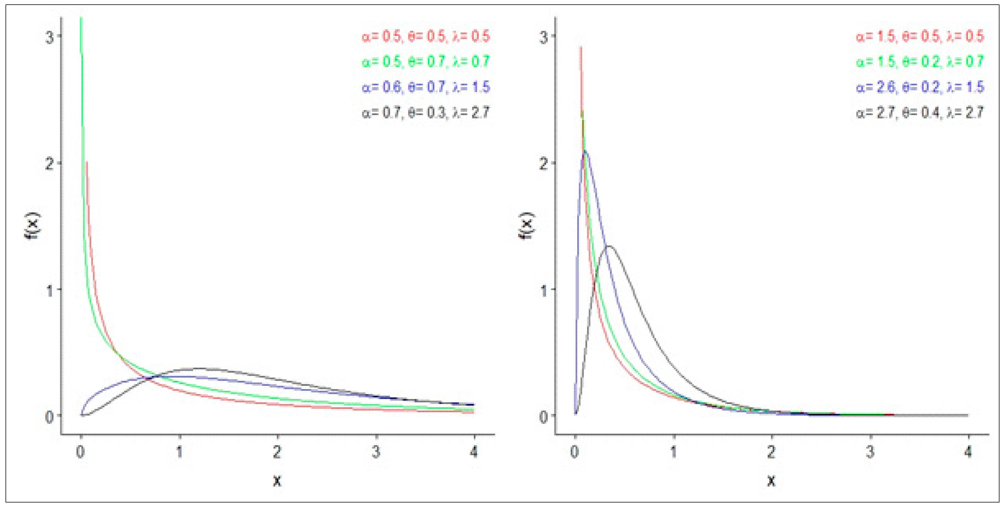
Figure 1. Plots of the probability density function (PDF) of EBE distribution.
Symmetry 12 01338 g001
Figure 2. Plots of the HRF of the EBE distribution.
Symmetry 12 01338 g002
Figure 3. Three-dimensional plot for the skewness of the EBE model.
Symmetry 12 01338 g003
Figure 4. Three-dimensional plot for the kurtosis of the EBE model.
Symmetry 12 01338 g004
Figure 5. Kernel density estimation and box plots.
Symmetry 12 01338 g005
Figure 6. Fitted PDF (left panel) and fitted cumulative distribution function (CDF) (right panel).
Symmetry 12 01338 g006
Table 1. Moments, skewness and kurtosis of the EBE model.
αθλμ1μ2μ3μ4SkewnessKurtosis
0.50.50.51.0663.00916.07149.7552.75212.349
0.50.70.71.6604.31323.29277.5092.1899.1470
0.60.71.52.4144.00814.47125.2781.6696.8000
0.70.32.72.2732.7498.14860.48101.6276.6450
1.50.50.50.2430.3160.5451.589002.75312.231
1.50.20.70.3810.2940.4581.269002.53911.139
2.60.21.50.4040.1490.1210.233001.9298.0020
2.70.42.70.6260.1950.1530.325001.5716.3250
Table 2. Mean square errors (MSEs) for n = 50, 100, 200, 500 and 1000.
n λαθMSEs
50 0.50.50.50.11892, 0.23647, 0.06169
100 0.08304, 0.17158, 0.04192
200 0.05794, 0.12764, 0.02949
500 0.03636, 0.08476, 0.01866
1000 0.02595, 0.06105, 0.01325
50 0.50.70.70.08813, 0.17030, 0.08578
100 0.06136, 0.11879, 0.05894
200 0.04320, 0.08131, 0.04139
500 0.02764, 0.04874, 0.02616
1000 0.01964, 0.03346, 0.01856
50 0.60.71.50.06866, 0.12976, 0.18044
100 0.04885, 0.08743, 0.12657
200 0.03427, 0.06270, 0.08909
500 0.02180, 0.03709, 0.05538
1000 0.01550, 0.02515, 0.03903
50 0.70.32.70.07211, 0.13178, 0.29484
100 0.05105, 0.09550, 0.20625
200 0.03537, 0.07094, 0.14854
500 0.02227, 0.04645, 0.09524
1000 0.01545, 0.03457, 0.06935
50 0.50.50.50.11892, 0.23647, 0.06169
100 0.08304, 0.17158, 0.04192
200 0.05794, 0.12764, 0.02949
500 0.03636, 0.08476, 0.01866
1000 0.02595, 0.06105, 0.01325
Table 3. Biases for n = 50, 100, 200, 500 and 1000.
n λαθMSEs
50 0.50.50.50.18356, 0.31326, 0.06034
100 0.14037, 0.29166, 0.02491
200 0.10718, 0.27047, 0.00952
500 0.07427, 0.22547, 0.00392
1000 0.05854, 0.18297, 0.00431
50 0.50.70.70.13103, 0.32039, 0.16804
100 0.09571, 0.29243, 0.12804
200 0.07617, 0.25160, 0.11495
500 0.05278, 0.17909, 0.10177
1000 0.03559, 0.11151, 0.09647
50 0.60.71.50.11728, 0.32816, 1.12796
100 0.09252, 0.29394, 1.03834
200 0.07715, 0.27919, 0.98811
500 0.05480, 0.21775, 0.91763
1000 0.03922, 0.17326, 0.88793
50 0.70.32.70.16086, 0.36788, 2.90744
100 0.13715, 0.35482, 2.70484
200 0.10661,0.32348, 2.66995
500 0.08491, 0.27404, 2.64048
1000 0.07009, 0.22686, 2.72810
50 0.50.50.50.18356, 0.31326, 0.06034
100 0.14037, 0.29166, 0.02491
200 0.10718, 0.27047, 0.00952
500 0.07427, 0.22547, 0.00392
1000 0.05854, 0.18297, 0.00431
Table 4. Average values (AVs) for n = 50, 100, 200, 500 and 1000.
n λαθMSEs
50 0.50.50.50.55465, 0.50616, 0.52281
100 0.53818, 0.51109, 0.50207
200 0.52237, 0.48520, 0.49930
500 0.50325, 0.47041, 0.49911
1000 0.49813, 0.46471, 0.50127
50 0.50.70.70.50550, 0.58874, 0.72531
100 0.49190, 0.60765, 0.70470
200 0.48878, 0.63157, 0.69991
500 0.49378, 0.66331, 0.69945
1000 0.49624, 0.67996, 0.70161
50 0.60.71.50.57701, 0.58491, 1.52331
100 0.58530, 0.61671, 1.51090
200 0.57826, 0.61435, 1.50499
500 0.58310, 0.65758, 1.47994
1000 0.58988, 0.68285, 1.47548
50 0.70.32.70.74776, 0.45747, 2.49293
100 0.74369, 0.44427, 2.46686
200 0.72548, 0.39578, 2.51294
500 0.71662, 0.36901, 2.54710
1000 0.70309, 0.31662, 2.62308
50 0.50.50.50.55465, 0.50616, 0.52281
100 0.53818, 0.51109, 0.50207
200 0.52237, 0.48520, 0.49930
500 0.50325, 0.47041, 0.49911
1000 0.49813, 0.46471, 0.50127
Table 5. Estimated average lengths (EALs) for n = 50, 100, 200, 500 and 1000.
n λαθMSEs
50 0.50.50.50.46616, 0.92696, 0.24180
100 0.32550, 0.67258, 0.16431
200 0.22713, 0.50034, 0.11560
500 0.14251, 0.33226, 0.07314
1000 0.10172, 0.23930, 0.05195
50 0.50.70.70.34545, 0.66757, 0.33625
100 0.24054, 0.46565, 0.23104
200 0.16935, 0.31873, 0.16226
500 0.10834, 0.19105, 0.10255
1000 0.07700, 0.13116, 0.07274
50 0.60.71.50.26914, 0.50864, 0.70733
100 0.19150, 0.34271, 0.49614
200 0.13434, 0.24579, 0.34924
500 0.08545, 0.14539, 0.21710
1000 0.06077, 0.09860, 0.15300
50 0.70.32.70.28268, 0.51657, 1.15574
100 0.20011, 0.37434, 0.80847
200 0.13865, 0.27809, 0.58226
500 0.08730, 0.18209, 0.37332
1000 0.06055, 0.13552, 0.27184
50 0.50.50.50.46616, 0.92696, 0.24180
100 0.32550, 0.67258, 0.16431
200 0.22713, 0.50034, 0.11560
500 0.14251, 0.33226, 0.07314
1000 0.10172, 0.23930, 0.05195
Table 6. Coverage probabilities (CPs) for n = 50, 100, 200, 500 and 1000.
n λαθMSEs
50 0.50.50.50.82686, 0.71564, 0.79176
100 0.76642, 0.65414, 0.75986
200 0.69834, 0.57143, 0.79418
500 0.66517, 0.51762, 0.82334
1000 0.57302, 0.51648, 0.81022
50 0.50.70.70.81610, 0.73529, 0.76823
100 0.78664, 0.58513, 0.72796
200 0.73695, 0.52505, 0.62213
500 0.72222, 0.47172, 0.60909
1000 0.74675, 0.49449, 0.61361
50 0.60.71.50.73690, 0.54738, 0.00000
100 0.70523, 0.40712, 0.00000
200 0.65622, 0.34796, 0.00000
500 00.6434, 0.28687, 0.00000
1000 0.65265, 0.25726, 0.00000
50 0.70.32.70.63454, 0.50188, 0.00000
100 0.51110, 0.28606, 0.00000
200 0.42228, 0.23378, 0.00000
500 0.31797, 0.22104, 0.00000
1000 0.29115, 0.20381, 0.00000
50 0.50.50.50.82686, 0.71564, 0.79176
100 0.76642, 0.65414, 0.75986
200 0.69834, 0.57143, 0.79418
500 0.66517, 0.51762, 0.82334
1000 0.57302, 0.51648, 0.81022
Table 7. The MLE for all the models corresponds to the failure times data set.
ModelEstimates
Burr Xa
0.462891
Burr XIIab
1.145711.94994
ELLGab
1.2116590.570392
BLLGabc
0.5816501.0919291.295956
EBEαθλ
0.8036090.0010.999053
BLLGWabcαβ
6.4680975.076580.223720.244630.93981
BWLLGabcαβ
0.707730.153111.457795.741920.72356
Table 8. Statistics for failure times of Kevlar data set.
Model−2 logL C [ 1 ] C [ 2 ] C [ 3 ] C [ 4 ]
EBE143.3996149.4100152.3784152.3784149.6087
Burr XII145.4801149.4801154.4119152.4660149.6229
BLLGW204.0771214.0771227.1527219.3705214.7087
BWLLG204.8205214.8205227.8961220.1139215.4521
Burr X285.8730287.8730290.3389288.8659287.9200
ELLG587.6830591.6830596.9133593.8004591.8055
BLLG462.1078468.1078175.9531471.2838468.3552

