Abstract
Apart from its applications in Chemistry, Biology, Physics, Social Sciences, Anthropology, etc., there are close relations between graph theory and other areas of Mathematics. Fibonacci numbers are of utmost interest due to their relation with the golden ratio and also due to many applications in different areas from Biology, Architecture, Anatomy to Finance. In this paper, we define Fibonacci graphs as graphs having degree sequence consisting of n consecutive Fibonacci numbers and use the invariant to obtain some more information on these graphs. We give the necessary and sufficient conditions for the realizability of a set D of n successive Fibonacci numbers for every n and also list all possible realizations called Fibonacci graphs for .
MSC:
05C07; 05C10; 05C30; 05C69
1. Introduction
Graph theory is one of the most popular subjects in mathematics as it can be applied to any area of science. One may easily found applications of graphs in networks, physics, electronical engineering, chemistry, molecular biology, pharmacology, transportation, trade, city planning, economy etc. Several mathematicians studied interrelations between number theory and graph theory and connected several properties of numbers with graphs. Every eigenvalue of a tree is a totally real algebraic integer and every totally real algebraic integer is a tree eigenvalue. So there is a close relation between algebraic number theory and spectral graph theory. In the network topology, for example in a hypercube convenient for parallel processing, the vertices are labeled with binary n-tuples if the hypercube is n dimensional. In [1], Erdös used graphs to prove a number theoretical inequality for the maximum number of integers less than a positive integer n no one of which divides the others. In this paper, we introduce graphs whose degree sequences consist of consecutive Fibonacci numbers and call them Fibonacci graphs.
The Fibonacci sequence is a famous number sequence whose name comes from the Italian Mathematician Leonardo Pisano, Fibonacci or Leonardo of Pisa lived between 1170–1240 in Italy. This number sequence is called Fibonacci sequence. Let be the r-th Fibonacci number. Taking as initial conditions, these numbers satisfy the recurrence relation for .
In [2], some graphs called Fibonacci cube graphs have been defined and studied. A Fibonacci cube graph of order n is a graph on vertices labeled by the Zeckendorf representations of the numbers 0 to so that two vertices are connected by an edge iff their labels differ by a single bit, i.e., if the Hamming distance between them is exactly 1. Note that our definition of Fibonacci graph of order n means a graph with n vertices with degrees equal to n successive Fibonacci numbers.
The rest of the paper is organized as follows. In Section 2, the necessary definitions and results related to invariant are recalled. In Section 3, the so-called Fibonacci graphs of order 1 to 4 are catalogued and their properties are studied. For an arbitrary non-negative integer n, the necessary and sufficient conditions for the existence of a Fibonacci graph of order n are established. The number of loops which is equal to the number of faces of the graph is formulized in all cases by means of the invariant.
2. Fundamentals and Invariant
Let be a graph of order n and size m. Let the degree of a vertex be denoted by . A vertex with vertex degree one is called a pendant vertex and an edge having a pendant vertex is similarly called a pendant edge. The biggest vertex degree is denoted by . A well-known result known as the handshaking lemma states that the sum of vertex degrees in any graph is equal to twice the number of edges of the graph. If u and v are two adjacent vertices of G, then the edge e between them is denoted by and also the vertices u and v are called adjacent vertices. The edge e is said to be incident with u and v. A support vertex is a vertex adjacent to a pendant vertex. If there is a path between every pair of vertices, then the graph is called connected.
In many cases, we classify our graphs according to the number of cycles. A graph having no cycle is called acyclic. For example, all trees, paths, star graphs are acyclic. A graph which is not acyclic will be called cyclic. If a graph has one, two, three cycles, then it is called unicyclic, bicyclic and tricyclic, respectively.
A loop is an edge starting end ending at the same vertex. Two or more edges connecting the same pair of vertices are called multiple edges. A graph is called simple if there are no loops nor multiple edges. Usually, simple graphs are preferable in many research, but in this work we shall make use of graphs with small order and much larger size making those graphs non-simple.
Considered with multiplicities, a degree sequence is written as
where ’s are positive integers corresponding to the number of vertices of degree . It is also possible to state a degree sequence as
where some of ’s could be zero.
Let be a set of non-decreasing non-negative integers. If there exists a graph G with degree sequence D, then D is said to be realizable and G is a realization of D. There is no formula for the number of realizations of a degree sequence and it is known that this number is quite big. The most well-known and effective results to determine the realizability are Havel-Hakimi and Erdös-Gallai, see [3,4]. There are some other techniques as well.
The degree sequence of some frequent graphs are as follows: , , , , and .
In this paper, we utilize some graph classes with one, two, three or four vertices. The ones with one and two vertices were defined and used in solving the problem of finding the maximum number of components amongst all realizations of a given degree sequence in [5]. A graph having q loops at a single vertex is denoted by . Some ’s are seen in Figure 1:
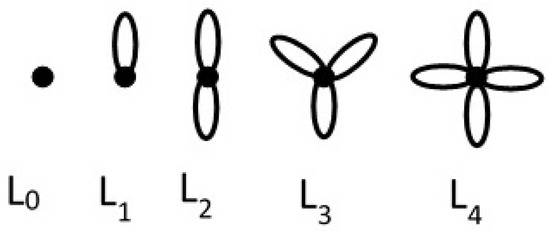
Figure 1.
Some graphs.
Let . is the graph having r loops at one end of an edge and s loops at the other. Some graphs are seen in Figure 2:
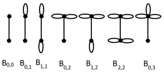
Figure 2.
Some graphs.
A connected graph having three vertices of degrees , and with are integers, respectively, is a graph consisting of a path such that a loops are incident to u, b loops are incident to v and c loops are incident to w. It will be denoted by , see Figure 3.
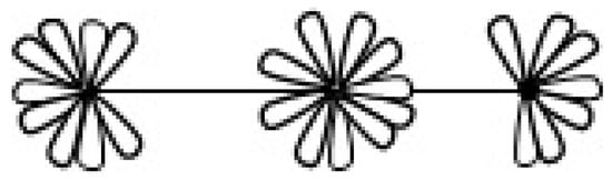
Figure 3.
.
A connected graph of four vertices having degrees , , and with are integers, is a graph consisting of a path so that a loops are incident to u, b loops are incident to v, c loops are incident to w and d loops are incident to z. It is denoted by , see Figure 4.
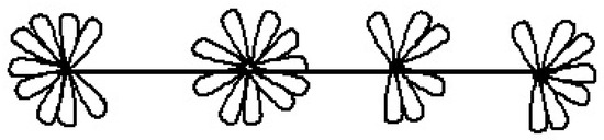
Figure 4.
.
For non-negative integers r and k, the notation “” will mean that k loops are attached at a new vertex on one of the r loops incident to others. For non-negative integers , the notation “” will mean that loops are attached to one of the loops of degree r at a new vertex, loops are attached to another loop of degree r at a another new vertex, and continuing this way, loops are attached to yet another one of the loops of degree r at another new vertex. Finally, the notation “” will mean that loops are attached to one of the loops of degree r at a new vertex, loops are attached to the same loop at a another new vertex, and continuing this way, loops are attached to the same loop at another new vertex. To illustrate the definitions, the notations , and corresponds to graphs shown in Figure 5, Figure 6 and Figure 7:
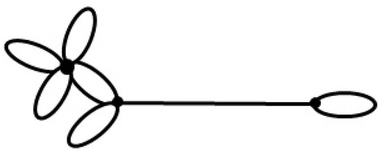
Figure 5.
The graph .
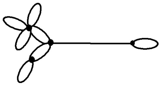
Figure 6.
The graph .
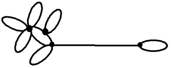
Figure 7.
The graph .
The following fact on Fibonacci numbers will be frequently used in this paper:
Observation 1.
Fibonacci numbers follows the rule odd, odd, even, odd, odd, even, ⋯. That is, the index r of a Fibonacci numberis divisible by 3, thenis even.
Fibonacci numbers have several interesting properties and there are a lot of identities about them. For example, there is a formula for the sum . This formula is given in the following result:
Theorem 1.
[6] The sum of the first r Fibonacci numbers satisfy the following equality
Some obvious consequences of this result are below:
Corollary 1.
(i).(ii).
We shall call a graph a Fibonacci graph if all its vertex degrees are consecutive Fibonacci numbers. We shall study the existence of Fibonacci graphs where the degree sequence has 1, 2, 3 or 4 elements.
Let G be a realization of a degree sequence D. We recall the definition and some properties of from [5,7,8,9,10]. The number of leaves of a tree T is
where is the number of vertices of degree i. Note that Equation (1) can be reformulized as
Generalizing this equation, is defined in [7] as follows:
Definition 1.
Letbe the degree sequence of a graph G. Theof G is defined in terms of D as
invariant of a tree T, path graph , cycle graph , star graph , complete graph , tadpole graph and complete bipartite graph where in the latter two cases are
Note that the fact invariant of a path, star or a tree is is true for all connected acyclic graphs as stated in [7].
We recall some basic properties of invariant. In most cases, we face with some disconnected graphs. The following result shows the additivity of invariant:
Theorem 2.
[7] Let G be a disconnected graph with c components. Then
The following relation is a useful tool in finding of a given graph G and is used frequently:
Theorem 3.
That is, invariant is always even. Hence, if is an odd integer for any set D of non-negative integers, as a new realizability test, we can conclude that D is not realizable.[7] For any graph G,
The number r of independent cycles in a connected graph G which is well-known as the cyclomatic number of G can be stated in terms of invariant:
Theorem 4.
[7] Let. If D is realizable as a connected planar graph G, then the number r of faces (closed regions) is given by
This result is used in many applications. The following is a generalization to disconnected graphs:
Corollary 2.
[7] Letbe realizable as a graph G with c components. The number r of faces of G is given by
In [5], the maximum possible number of components amongst all realizations of a degree sequence was given by the formula
In any graph, there are edges, vertices and faces. These three graph parameters frequently appear as bridges, cut vertices, pendant vertices, chords, loops, multiple edges, pendant edges, etc. For the fundamental notions in Graph Theory, see [11,12,13,14,15].
3. Existence Conditions for Fibonacci Graphs
In this section, we show the existence of graphs with n consecutive Fibonacci numbers as their vertex degrees. That is, we are looking for graphs with degree sequence consisting of n consecutive Fibonacci numbers. This problem can be restated as follows: Which sets having n consecutive Fibonacci numbers are realizable as graphs? We shall solve this problem by means of the invariant.
3.1. Fibonacci Graphs of Order 1
We now start with the Fibonacci graphs of 1 vertex. These are the graphs consisting of a single vertex with degree a Fibonacci number.
Theorem 5.
A graph with one vertex is a Fibonacci graph if and only if its size isfor some positive integer k. In this case, the graph is.
Proof.
Let a graph G with one vertex be of size . Then as there is only one vertex, say v, all ends of the edges are v. Therefore the degree of v is twice which is and this shows that the graph is a Fibonacci graph.
Let G be a Fibonacci graph with one vertex v. As G is a Fibonacci graph, for some positive integer r. The sum of vertex degrees which is equal to the degree of v must be even. Therefore must be even which is possible when r is divisible by 3. □
In such a case, the degree sequence of this graph having one vertex must be . Hence, its realization would be the graph and . Hence all Fibonacci graphs of order 1 may have 1, 4, 17, 72, 305 faces, that is, they are , , , , , ⋯, , ⋯. Therefore we showed
Corollary 3.
A graph with one vertex is a Fibonacci graph iff it hasfaces for some positive integer k.
3.2. Fibonacci Graphs of Order 2
We now discuss the Fibonacci graphs having two vertices. Namely, we want to find which sets consisting of two consecutive Fibonacci numbers are realizable. By the Observation 1, only the Fibonacci numbers are even. So to have and as the vertex degrees of a Fibonacci graph having two vertices, the graph must be connected and also we must have . That is, the degrees of the vertices must be and for some integer k. If the graph is disconnected, then two components must have orders and . But this is a contradiction with the Handshaking Lemma. Therefore, we proved
Theorem 6.
A graph with two vertices is a Fibonacci graph iff its degree sequence isfor some integer k.
In this case, the graph is with invariant
Hence
This proves the following:
Corollary 4.
If a graph of order 2 is a Fibonacci graph, then it hasfaces for some integer k.
Note that the converse may not be true.
For , the vertex degrees are and and by Equation (3), the maximum number of components is
Therefore there is only one connected graph given in Figure 8:
Figure 8.
The Fibonacci graph having vertex degrees and .
This graph is and by Equation (4), there are faces, implying that the graph is acyclic.
For , the vertex degrees are and . Similarly to the above, there is only one connected graph given in Figure 9:
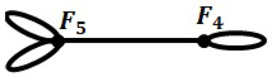
Figure 9.
The Fibonacci graph having vertex degrees and .
This graph is . Note that by Equation (4), there are faces in .
In summary, when , for each non-negative integer k, the only connected Fibonacci graphs are and each of them has loops at one end, loops at the other end and faces.
3.3. Fibonacci Graphs of Order 3
Now we take Fibonacci graphs with three vertices. Note that, the sum of three consecutive Fibonacci numbers is always even, implying the following result:
Theorem 7.
Every degree sequence consisting of any three consecutive Fibonacci numbers is realizable as a Fibonacci graph.
So there are three possibilities for the degree sequence of such a graph where k is a non-negative integer: , or . In each of these cases, we have one even and two odd integers. Hence, the maximum number of components is
A Fibonacci graph with three vertices can be connected or may have two components. This is because there are two odd degrees and an even one. A realization of 3 components is impossible as two components would have total vertex degree odd. So, for the three degree sequences above, two odd degree vertices must belong to the same component, and the other vertex could belong to this component causing a connected graph, or could form a second component. We now consider these possibilities:
Case 1.
First letIn this case, Ω of D is
As is even, D is always realizable by Theorem 3. For the case of where ,, the only possible connected realization is in Figure 10:
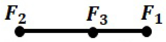
Figure 10.
The unique connected realization of .
which is a path graph which has faces. The unique disconnected realization of D is given in Figure 11:
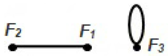
Figure 11.
The unique disconnected realization of .
which is the graph (or ) and it has faces, i.e., it is unicyclic.
Let us now consider for . By the above discussion, it is not difficult to determine the existence of the following three connected realizations of D given in Figure 12:
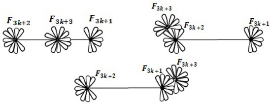
Figure 12.
All three connected realizations of .
which are , and , respectively. In all these graphs, the number of faces is . The fourth and final realization of D is a disconnected graph in Figure 13 which has faces.
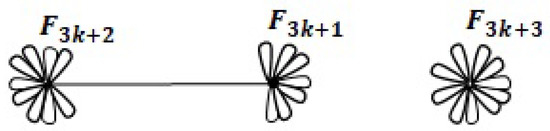
Figure 13.
The unique disconnected realization of .
Case 2.
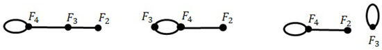
Let us secondly take. We haveNote thatandare odd andis even. In the singular case ofwhere three consecutive Fibonacci numbers are, there are three possible graphs as below: two are connected and one is disconnected. The first and second graphs in Figure 14 have the number of faces 1 which is compatible with Theorem 4 and the third graph has 2 faces which is compatible with Corollary 2. These graphs are named by,and, respectively.
Figure 14.
All three realizations of .
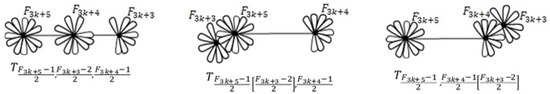
Now, we take D as a set of three consecutive Fibonacci numbers , , for . There are four graph realizations, three are connected, see Figure 15, and one is disconnected, see Figure 16. The connected ones are
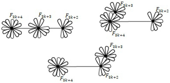
Figure 15.
All three connected realizations of .
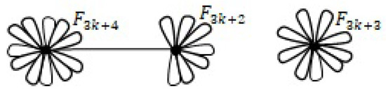
Figure 16.
The unique disconnected realization of .
which are respectively denoted by , and finally by which all have faces. Finally, there is a disconnected realization of D given in Figure 16: which is denoted by . It has faces.
Case 3.
If we take. Then similarly,We have no singular case and there are four realizations, the first three are connected and the last one is disconnected. The connected realizations are in Figure 17.
Figure 17.
All three connected realizations of .
They all have faces. Also, there is a disconnected realization with faces given in Figure 18.
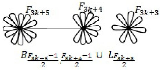
Figure 18.
The unique disconnected realization of .
We have the following generalization:
Corollary 5.
For a positive integer s, every set consisting of consecutiveFibonacci numbers is realizable as a Fibonacci graph of order.
3.4. Fibonacci Graphs of Order 4
Finally, we discuss the case of . We want to have a degree sequence with four consecutive Fibonacci numbers to be realizable. We have
Theorem 8.
Letbe four consecutive Fibonacci numbers.
is realizable iff r is a multiple of 3.
Proof.
Let us take four consecutive Fibonacci numbers . The sum of these numbers must be even. If E denotes an even number and O denotes an odd one, by Observation 1.1, the possible sums are E+O+O+E, O+O+E+O or O+E+O+O when or , respectively. Therefore the result.
If r is a multiple of 3, then and are even and and are odd giving the realizability of D. □
Hence, the only possible degree sequence for a Fibonacci graph of order 4 is
for a positive integer k. For such a degree sequence, is even implying that D is realizable by Theorem 3. Also
That is, any realization of D might have at most three components.
If we take , we get and we would have realizations having one, two or three components. The fourteen connected realizations are , , , , , , , , , , , , , . There are seven disconnected realizations with two components which are , , , , , , , and finally there is a unique disconnected realization with three components . In general case where , we have eighteen connected realizations
seven disconnected realizations
having two components, and a unique disconnected realization with three components.
3.5. Fibonacci Graphs of Order
In the above four subsections, we established the conditions for a set of n consecutive Fibonacci numbers to be realizable where , and generalized these to sets of length . Therefore, only two cases where and remains:
Corollary 6.
(i) A setconsisting ofconsecutive Fibonacci numbers is realizable iff. (ii) A setconsisting ofconsecutive Fibonacci numbers is realizable iff.
Author Contributions
Conceptualization, I.N.C., A.S.C. and S.D.; methodology, A.Y.G. and M.D.; writing—original draft preparation, M.D.; visualization, M.D. and A.S.C.; supervision, I.N.C. All authors have read and agreed to the published version of the manuscript.
Funding
No external funding.
Conflicts of Interest
We declare no conflict of interest.
References
- Erdös, P. On some applications of graph theory to number theoretic problems. Publ. Ramanujan Inst. 1969, 1, 131–136. [Google Scholar]
- Hsu, W.-J.; Page, C.V.; Liu, J.-S. Fibonacci Cubes: A Class of Self-Similar Graphs. Fib. Quart. 1993, 31, 65–72. [Google Scholar]
- Hakimi, S.L. On the realizability of a set of integers as degrees of the vertices of a graph. J. SIAM Appl. Math. 1962, 10, 496–506. [Google Scholar] [CrossRef]
- Havel, V. A remark on the existence of finite graphs (Czech). Časopic Pěst. Mat. 1955, 80, 477–480. [Google Scholar]
- Delen, S.; Cangul, I.N. Extremal Problems on Components and Loops in Graphs. Acta Math. Sin. Engl. Ser. 2019, 35, 161–171. [Google Scholar] [CrossRef]
- Koshy, T. Fibonacci and Lucas Numbers with Applications; John Wiley and Sons: New York, NY, USA, 2001. [Google Scholar]
- Delen, S.; Cangul, I.N. A New Graph Invariant. Turk. J. Anal. Number Theory 2018, 6, 30–33. [Google Scholar] [CrossRef][Green Version]
- Delen, S.; Togan, M.; Yurttas, A.; Ana, U.; Cangul, I.N. The Effect of Edge and Vertex Deletion on Omega Invariant. Appl. Anal. Discr. Math. 2020, 2020, 14. [Google Scholar]
- Delen, S.; Yurttas, A.; Togan, M.; Cangul, I.N. Omega Invariant of Graphs and Cyclicness. Appl. Sci. 2019, 21, 91–95. [Google Scholar]
- Sanli, U.; Celik, F.; Delen, S.; Cangul, I.N. Connectedness Criteria for Graphs by Means of Omega Invariant. FILOMAT 2020, 34, 2. [Google Scholar]
- Bondy, J.A.; Murty, U.S.R. Graph Theory; Springer: New York, NY, USA, 2008. [Google Scholar]
- Diestel, R. Graph Theory; Springer GTM: New York, NY, USA, 2010. [Google Scholar]
- Foulds, L.R. Graph Theory Applications; Springer Universitext: New York, NY, USA, 1992. [Google Scholar]
- Wallis, W.D. A Beginner’s Guide to Graph Theory; Birkhauser: Boston, MA, USA, 2007. [Google Scholar]
- West, D.B. Introduction to Graph Theory; Pearson: Delhi, India, 2001. [Google Scholar]
© 2020 by the authors. Licensee MDPI, Basel, Switzerland. This article is an open access article distributed under the terms and conditions of the Creative Commons Attribution (CC BY) license (http://creativecommons.org/licenses/by/4.0/).