1. Introduction
Currently, artificial intelligence is taking a greater role in the various processes of automation. Mining has not been elusive, having developed different models of Artificial Neural Networks (ANN) for prediction in the area of blasting. Within studies published on this subject, Oraee and Asi [
1] mentioned that breakage of the rock after blasting is an important factor in the associated cost of the mine. In this work, we find that the breakage of the rock after blasting is estimated analytically using the neural networks. This study was carried out using the actual data collected from the Gol-e-Gohar iron mine in Iran. Kulatilake et al. [
2] developed a prediction model for rock fragmentation based on ANN, in order to predict the average size of the particles, resulting from fragmentation in rock blasting. In their work, the authors considered four learning algorithms to train neural network models. The authors concluded that the neural network model obtains greater accurate results than the empirical models.
However, the studies by Shi et al. [
3] mentioned that, to solve the problems with regard to the inaccuracy in predicting the traditional method of assessing particle size distribution in blasting, Support Vector Machines (SVM) are used to predict the average particle size resulting from rock breakage in blasting. The prediction results using SVM were compared with those of ANN, concluding that the SVM method is quite accurate and provides a new way of predicting rock-blasting breakage. Then Gao and Fu [
4] developed an ANN model to predict the distribution of rock breakage in a Tantalum–Niobium mine achieving satisfactory results, which favored the selection of blasting parameters and an improvement in production.
In studies conducted in a limonite quarry by Sayadi et al. [
5] compared the application of several ANN with multivariate regression methods to develop a model for predicting rock breakage based on 103 shot records, concluding that ANN offer greater accuracy in predictions, these studies were conducted in Tehran, Iran. Then in Mohamad et al. [
6] stated that rock blasting is the most common method of rock excavation in quarries and surface mines. Blasting has some environmental consequences, such as: soil shaking, air gust, dust, fumes and rock. One of the most undesirable phenomena in the blasting operation is flyrock, which is a fragment of rock propelled by explosive energy beyond the area of the explosion. The prediction of the distance and size of the rocks thrown is a remarkable step in the reduction and control of blasting accidents in the operations, for this the authors used ANN to predict the distance and size of the rocks thrown in the blasting operations, the results obtained show that this technique is applicable for such prediction. This work was developed in a granite quarry located in Malaysia.
Independently, Saadat et al. [
7] developed a model for blasting for rock-induced vibration prediction using ANN that were compared with empirical and multiple regression analysis models. From this, the authors obtained better results of
and Mean Square Error (MSE) using the ANN model. In their research, the authors used 69 records acquired from an iron mine at Go-e-Gohar, Iran. In Marto et al. [
8] developed a predictive model about Fly Rock originated because of blasting in an aggregate quarry. In their research, they applied a combination of Artificial Neural Networks and the Imperialist Competitive Algorithm (ICA-ANN) which was later compared with the empirical models, multiple regression analysis and backpropagation ANN. The data used in this study were collected from a quarry in Malaysia where the prediction model proposed by the authors have got a
higher than the other models.
The work of Enayatollahi et al. [
9] compared two methods, using ANN and regression models in an investigation carried out in the Gol-e-Gohar iron mine. The authors concluded that the results obtained using ANN in the prediction of breakage resulting from blasting with respect to regression models are quite similar to those of reality. Independently Dhekne et al. [
10] made a synthesis of all the studies carried out with ANN to predict breakage and concluded that these models have distinct advantages such as flexibility, non-linearity, higher fault tolerance and adaptive learning over regression models.
In Tiile [
11], it was developed an ANN using 180 rock-blasting records in order to predict the following parameters: airblast, blast-induced ground vibration and rock fragmentation. The data used in this study were collected from a gold mine in Ghana and the model proposed by the authors have got the lower mean square error in comparison with the empirical and statistical models. Then, Taheri et al. [
12] proposed a hybrid model for the blasting of rock-caused vibration prediction. In their model, they combined the Artificial Neural Networks and the algorithm named Artificial Bee Colony (codename ABC-ANN). Artificial Bee Colony (ABC) was used as optimization algorithm to adjust the weights and bias of the artificial neural network, thereby achieving better performance than others models in terms of accuracy and generalization capacity. The data used in this study were obtained from a copper mine in Iran.
This evolutionary optimization algorithm was inspired by the social behavior of groups of insects and animals such as swarms of bees, flocks of birds, and shoals of fish [
13,
14]. Then in the publication of Dhekne et al. [
15] developed an ANN model to estimate the number of resulting rocks from explosions in limestone quarries at one of Indian Province. In their work they taken as a database three hundred explosions carried out in 4 limestone quarries that have a similar geotechnical classification.
In a limonite quarry, in Malaysia Murlidhar et al. [
16] a model hybrid was used based on Imperial Competitive Algorithm and Artificial Neural Network, in order to predict the breakage of rock through blasting, using as an input data diverse blasting parameters and characteristics of the rock mass. With the evaluation of the model mentioned before, the authors conclude that the proposed model is quite efficient to estimate the breakage of rocks. Then in Asl et al. [
17] developed a predictive model about Fly Rock and breakage of rock using an ANN model and the firefly algorithm. The authors have got a great performance on their model, obtaining satisfactory results of
and mean square error (MSE). The data used in this study were obtained from a limestone mine in Tajareh—Iran.
A study carried out in India by Das et al. [
18] developed a prediction of the shaking model for blasting with ANN, taking 248 blast registration from three coal mines with different geological conditions, geomechanical characteristics, blast parameters as well as the distance between the blast point and the shaking monitoring station to predict the Peak Particle Velocity (PPV), obtaining more accurate results than other empirical models. Finally, in Lawal and Idris [
19] developed a mathematical model based on ANN in order to predict blast-induced vibrations at a mine in Turkey, taking 14 records to be tested. The authors have got better results of
in comparison with the empirical models of Langefors-Kilhstrom and multiple regression analysis.
Based on all the above-mentioned studies, an Artificial Neural Networks (ANN) model of the multilayer perceptron type has been developed for the prediction of rock breakage using blasting. Taking the variables as data base involved in the drilling and blasting design, geomechanical properties of rock mass, explosives; which were the input data and the breakage results , and , defined with 80%, 50% and 20% of the throughput size in the crusher within open pit mine, were used for the output data formation of a network. For its development, Python programming language was used for the design of ANN, also using the gradient descent algorithm. The main reason that led us to conduct this work is the necessity to prove the high level of reliability of ANN, as well as the application of artificial intelligence in the different processes of the mining business. In addition, we will verify the feasibility in the use of single hidden layer in the ANN design, as well as demonstrate the good performance of the model, on the basis of the parameters of rocks, drilling and blasting as data input, to predict , and breakage sizes that in previous studies by different authors were not carried out.
The present work is divided up as follows, in
Section 2 the theoretical framework to be used, in
Section 3 we present the methodology to carry out the study, in
Section 4 we show collection of field data, in
Section 5 we explain the design and experimentation of the study, in
Section 6 we show the experimental results obtained and finally in
Section 7 the conclusions obtained from the present study.
2. Theoretical Frame
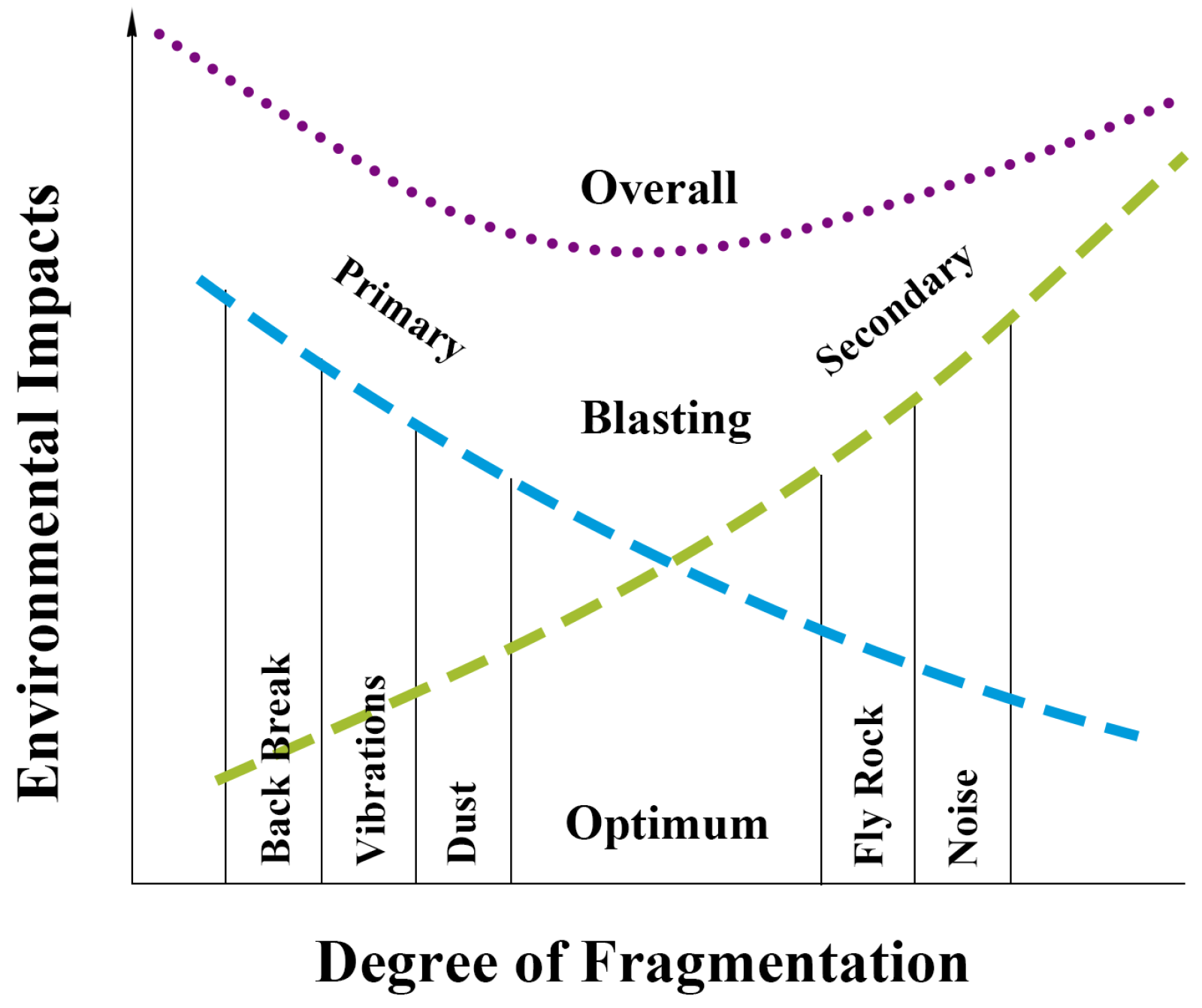
In rock blasting, rock breakage is one of the operations that requires a prior in-depth analysis. An adequate breakage has to take into account the variables to avoid inconveniences in the subsequent costs of loading, hauling, crushing and milling then it is important to know the variables that take a part in the drilling and blasting process, as well as the properties of the rock mass on which these activities are being performed, this are divided in two types of variables:
Controllable variables: Explosives, Geometric blasting design and Startup sequences.
Uncontrollable variables: Geological and Geomechanical characteristics of the rock mass.
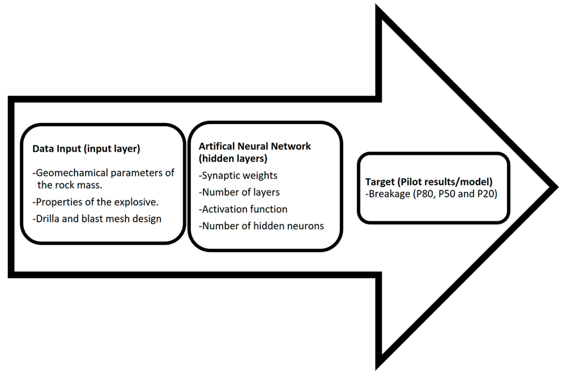
These variables are selected in a way that allow us to take advantage of the maximum energy of the explosive to obtain a breakage with which the performance of subsequent processes can be maximized, in other words, if the distribution of breakage is controlled, a significant improvement will be obtained in the yields and costs of subsequent operations within the process chain. This is why drilling and blasting are important in the process, as well as their results such as breakage, stack shape, bulking, dilution and microfracturing of the rock as they affect the efficiency of subsequent processes such as crushing and grinding, taking into account the environmental impacts that could lead to an adequate selection of breakage size, as can be seen in
Figure 1.
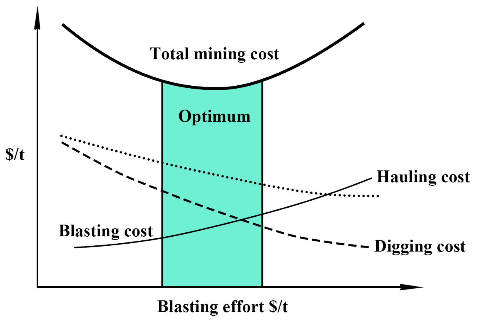
In operations where mining is merely moving the ore from one place to another, these processes have allocated budgets and production. Furthermore, the management carried out is aimed at maximizing production at minimum total cost of mining through the cost increase of breakage as shown in
Figure 2.
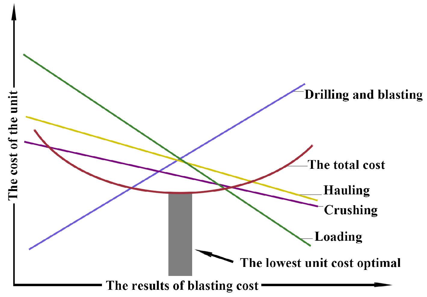
In most mining operations, it can be seen that the costs of crushing and grinding are relevant (40% to 60% of the total mine-grinding cost) so it is necessary to redistribute unit operations were they are more efficient and cheaper, such as after finding the most appropriate grain size distribution (through prediction models) commence optimizing of drilling and blasting designs so that the grain size distribution optimizes the performance of the subsequent rock treatment processes this could probably lead to increased drilling and blasting costs if necessary as shown in
Figure 3.
Exist empirical models that predict breakage taking into account these variables, such as the Kuz–Ram equation. Theoretically, Artificial Neural Networks (ANN) and Multiple Linear Regression (MLR) could also be used to predict this breakage.
2.1. Kuz–Ram Equation
Cunningham [
23,
24] modified the Kuznetsov equation [
25] in order to estimate the mean fragment size as well as using the Rosin–Rammler distribution [
26] to describe the complete size distribution. The final equation developed by Cunningham is known as the Kuz-Ram model and is shown in the Equation (
1):
where:
= Percentage of passing fragments less than 50%.
A = Rock factor.
= Explosive mass per drill.
E = Relative weight Strength of explosive
= Volume per kg of explosive.
2.2. Use of the Artificial Neural Network (Ann)
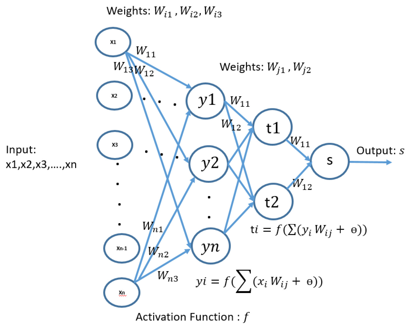
ANNs are composed of many simple interconnected processing elements called neurons or nodes. Each node receives an input signal with information from other nodes or external stimuli, processes it locally through an activation or transfer function and generate an output signal that is sent to other nodes or external outputs as shown in
Figure 4. Although a single neuron may seem extremely simple, the interconnection of several neurons that build a network is very powerful.
The main advantage of ANN is its ability to incorporate non-linear effects and interactions between model variables, with no need to include them a priori, as well as its ability to derive meaning from complicated or imprecise data. Recently, there has been a growing interest in obtaining adequate predictive models in mines. Among the possible alternatives available, Artificial Neural Networks are increasing used. In this paper we will use the most common type of ANN trained with Multilayer Perceptron algorithms (MLP).
2.3. Design of a Feedforward Neural Network (Fnn) for the Case Study
The correct design of an ANN typically consists of finding out the best configuration of the elements that make up its architecture. In our study, to determine the best architecture, we focus on the number of layers and the numbers of neurons in each layer, establishing the initial weights, the MLP transfer function, and considering previous studies to determine the best training algorithm for this kind of problem.
2.3.1. Number of Layers
For this particular case of the mine problem, three layers have been considered for our study.
2.3.2. Number of Neurons in Each Layer
The number of neurons per layer consist of 13 neurons in the hidden layer and one neuron in the exit layer.
2.3.3. Initialization of Weight
At initialization, we use random weights that are small enough around the origin for the activation function to work in its linear regime.
2.3.4. Activation Function of Each Layer
We use the sigmoid function that has the property of symmetry, defined in Equation (
2), as the activation of each layer:
where:
f: Sigmoid function
x: variable
2.3.5. Training Algorithm
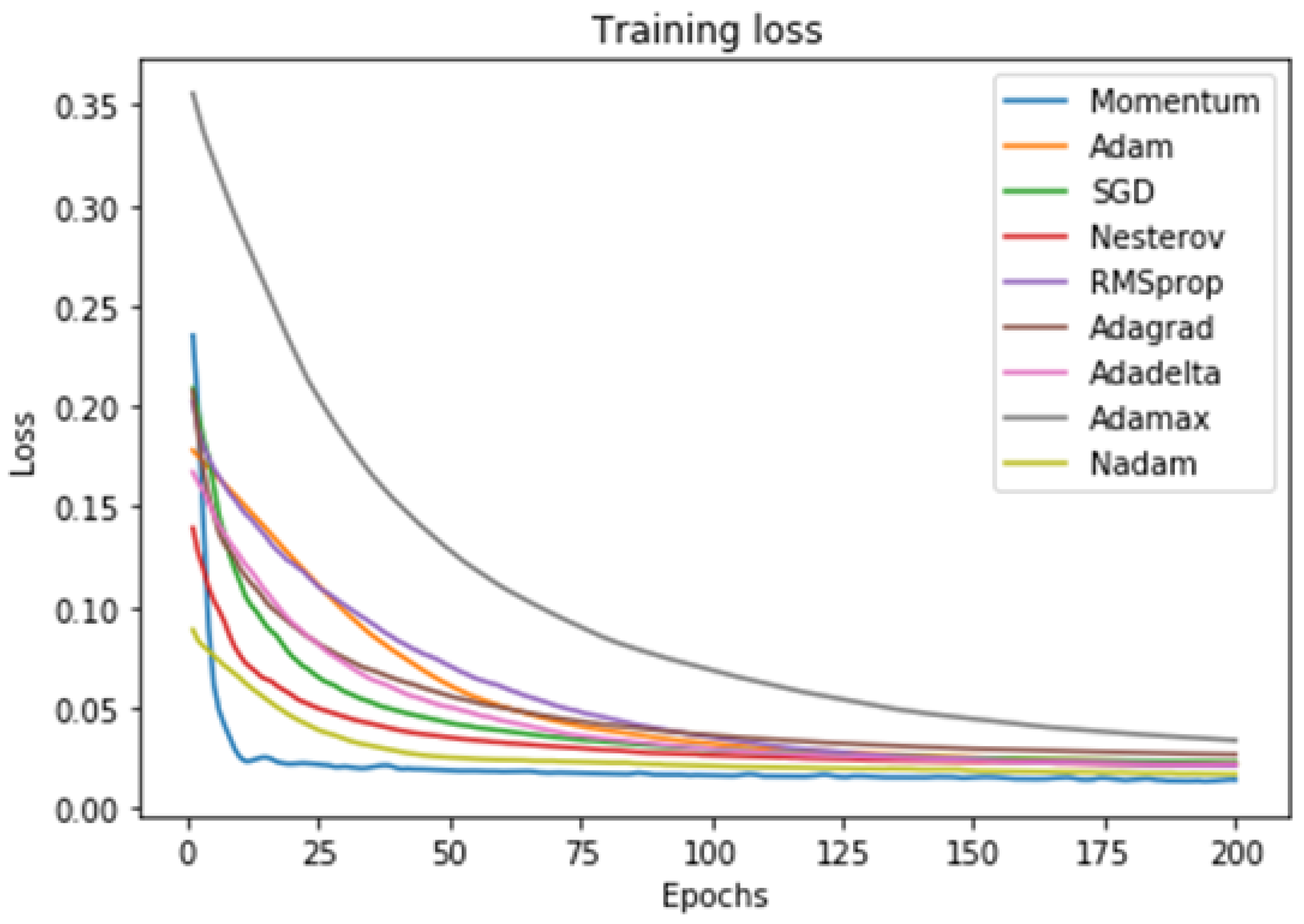
For the training and validation of the designed ANN, several descent algorithms were tested to find the convergence for optimal ANN. According to [
27] gradient descent algorithms are increasingly popular for performing the neural network optimization. In his study it mentions that there are several algorithms to optimize the gradient descent such as: Momentum, Nesterov, Adagrad, Adadelta, Adam, RMSprop, Adamax, and Nadam.
On that basis, with input data we conducted several tests with the mentioned algorithms to find out which one is the most acceptable. The result is that the Momentum algorithm (blue curve) is the most acceptable for our case, as shown in
Figure 5, reaching the global minimum before the other algorithms.
The Momentum algorithm, which we use, updates its weights through the Equation (
3):
where:
2.4. Multiple Linear Regression (Mlr)
Multiple linear regression [
28] allows the generation of a linear model in which the value of the dependent variable (
Y) is determined from a set of independent variables called predictors
. Multiple regression models can be used to predict the value of the dependent variable or to evaluate the influence that predictors have on it (the latter should be analyzed with caution so as not to misinterpret cause and effect). Multiple linear models follow Equation (
4):
where
: is the ordinate in the origin, namely is the value of the dependent variable Y when all the predictors are zero.
: is the average effect that the increase in one unit of the predictor variable has on the dependent variable Y, holding all else constant. This are known as partial regression coefficients.
: is the residual or error, namely the difference between the observed value and the one estimated by the model.
It is important to keep in mind that the magnitude of each partial regression coefficient depends on the units in which the predictor variable is measured apply, so its magnitude is not associated with the importance of each predictor. In order to determine what impact each variable has on the model, partial standardized coefficients are used, that are obtained through a standardizing process (subtracting the mean and dividing using the standard deviation) the predictor variables after adjusting the model. Based on the mentioned models and the available data, the study was carried out developing the multiple linear regression and ANN models, because of the data lacked the results predicted by the Kuz–Ram model. In the case of having the data from the Kuz–Ram model, the performance of ANN could be compared with the traditional method.
4. Collection of Field Data
Drilling and blasting parameters were taken from the study in [
29], which consists of 47 samples of blasting records made at a mine in northern Chile. These make up the following drilling and blasting parameters: Burden (B), Spacing (S), Bench Height (H), Stemming (T), Diameter (D), Kilograms of charged Explosives (Kg. Expl), Power Factor (PF), Geotechnical ore Units (GU), Overdrilling, Density of Explosive (D.Expl) and Mineral Density which corresponds to a classification of the rock mass as a function of uni-axial compressive strength, fracture frequency, density, etc. It is worth mentioning that 37 samples were taken for the training of the network and 10 for the respective testing. The following training parameters are shown in
Table 1:
The variables Burden, Spacing, Geotechnical ore Units, Mineral Density, Stemming, Density of Explosive, Kilograms of charged Explosives, Powder Factor were taken as input variables as well as , , as variables of output, since the Diameter, Overdrilling, and Bench parameters remain constant in data collection.
In the
Table 1, values of
,
, and
were obtained using image analysis method to determine size distribution which consist of three phases: selecting the sampling site, imaging, and image analysis. The sampling phase involves the selection of sites to obtain samples that represent the blasted rock mass. In the imaging phase, high quality images were selected, which can be analyzed in the analysis phase. In the last phase, the size distribution of fragments marked on the image is measured after drawing the perimeter of fragments on the image [
30].
5. Design and Experimentation of ANN
Once the input data is obtained, including geomechanical parameters of the rock, drilling and blasting design, explosives and the diameter of the breakage using blasting, we design the feed-forward neural network of the supervised type, considering the reliable and representative data avoiding the overfeeding of the ANN in order to achieve the desired learning. In the design of the architecture, we tested the number of layers and neurons that will make the ANN work properly for training using the data in
Table 1.
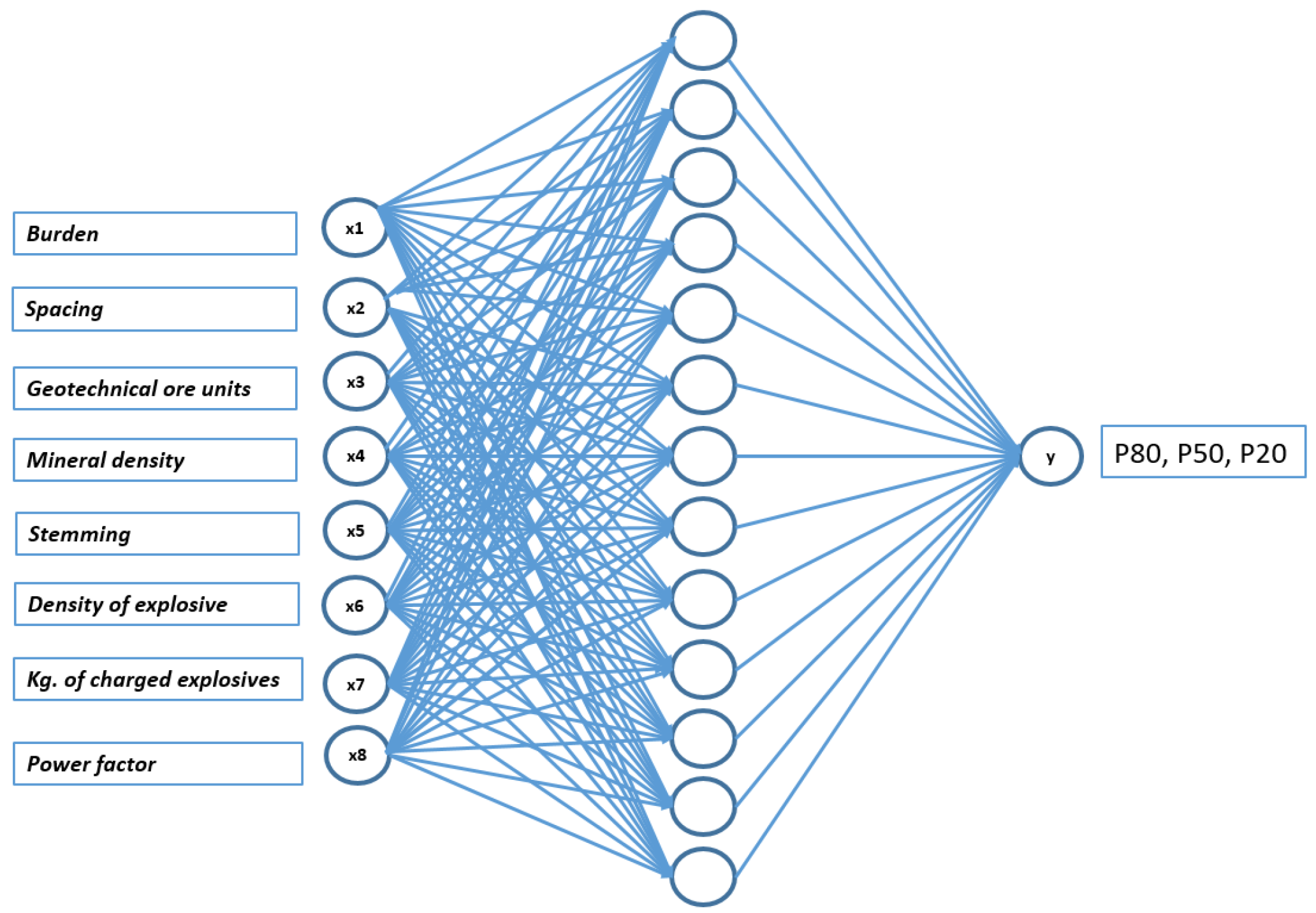
Figure 7 shows the diagram of the ANN design with a hidden layer.
To determine the number of hidden layers, we used the studies conducted by Cybenko [
31] which show that any continuous function can be uniformly approximated by single-layer hidden neural network models. The number of hidden layers and neurons in each layer affect the capacity of the model for generalization, i.e., the accuracy in computing new examples [
32].
Therefore, ANN in this work will only have a hidden layer as shown in
Figure 7. The number of neurons in the hidden layer is determined based on two empirical formulas: firstly Hecht–Nielsen [
33], based on the theorem of Kolmogorov [
34], suggests that 2
n + 1 (where “
n” is the number of input parameters) should be used as the maximum number of neurons for a hidden layer of a backpropagation network. Therefore, if the number of input parameters is
n = 8, the number of hidden neurons should be
N ≤ 17. Finally, according to a second empirical formula of Ge and Zu [
35], the number of neurons in the hidden layer must satisfy Equation (
5):
where:
n: number of input parameters = 8
K: used dataset number = 47
N: number of hidden neurons to be determined
Resulting N > 8. Therefore: 9 ≤ N ≤ 17.
These
N values were used to determine the appropriate functioning of ANN, and to establish its architecture, which was evaluated for each
N value, using two parameters; the root mean squared error and the correlation coefficient between predicted and actual values.
Figure 7 shows the summary of the ANN design together with the input and output parameters to be obtained.
6. Experimental Results and Discussion
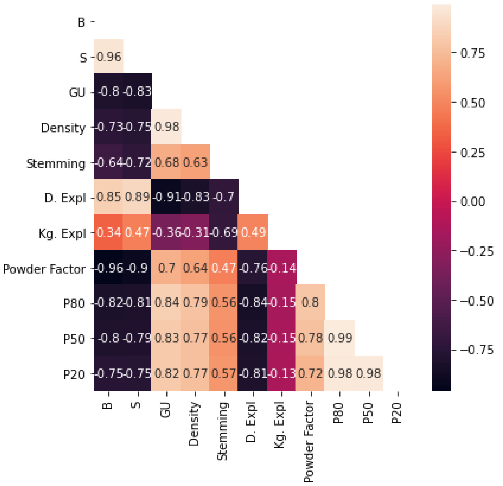
Next, we present the correlation matrix between the input and output parameters of the ANN, which allowed us to know the values of the Pearson’s correlation coefficients, which measure the degree of linear relationship between each pair of variables. The matrix is shown in
Figure 8.
These correlation values vary between [−1, +1]. If this coefficient is equal to 1 or −1 (or close to these values) it means that one variable is the product of a linear transformation of the other. There is a direct relationship when approaching 1 (when one variable increases, the other also increases), while there will be an inverse relationship when approaching −1 (when one variable decreases, the other also decreases). If the coefficient is equal to 0 (or close to this value) there is no linear relationship [
36].
Figure 8 shows the relationships between all the variables using colors. The darker the color, the linear relationship will be more negative between the variables. We observe negative correlations for the following parameters: Density of Explosive (D.Expl), Burden (B), Spacing (S) and Kilograms of charged Explosives (Kg.Expl) in the correlation matrix. Presenting these parameters values close to −1 in the mentioned order, inversely influencing the fragmentation results of
,
and
.
While the positive correlations in the parameters Geotechnical ore Unit (GU), Powder Factor, Mineral Density (Density) and Stemming, show a direct relationship in the fragmentation results. Being the variable GU the most predominant rock geotechnical parameter in the drilling and blasting process given the results of , and .
Once the ANN architecture model was designed, it was implemented, beginning with the training stage and then with the validation of the ANN. Therefore, with the values obtained previously, train then the ANN, minimizing the root mean squared error with the training data and the values of “n” (number of neurons in the hidden layer) using the Descending Gradient Algorithm over a number of 500 training cycles until the error is minimized.
Figure 9 shows the root mean square error, which stabilizes as ANN training cycles increase, using the Descending Gradient Algorithm, for both training (blue curve) and testing data (orange curve).
Analyzing
Figure 9, and
Table 2 gained from ANN simulations, (which presents the root mean square error values for each number of neurons obtained during network training using 500 cycles), it is determined that with
n = 13 we get a lower root mean squared average error (0.009557). Therefore, we use
n = 13 in the ANN for the predictions of
,
and
. Then, we proceeded to compare them using training and testing data, and got the following results which we discuss on below:
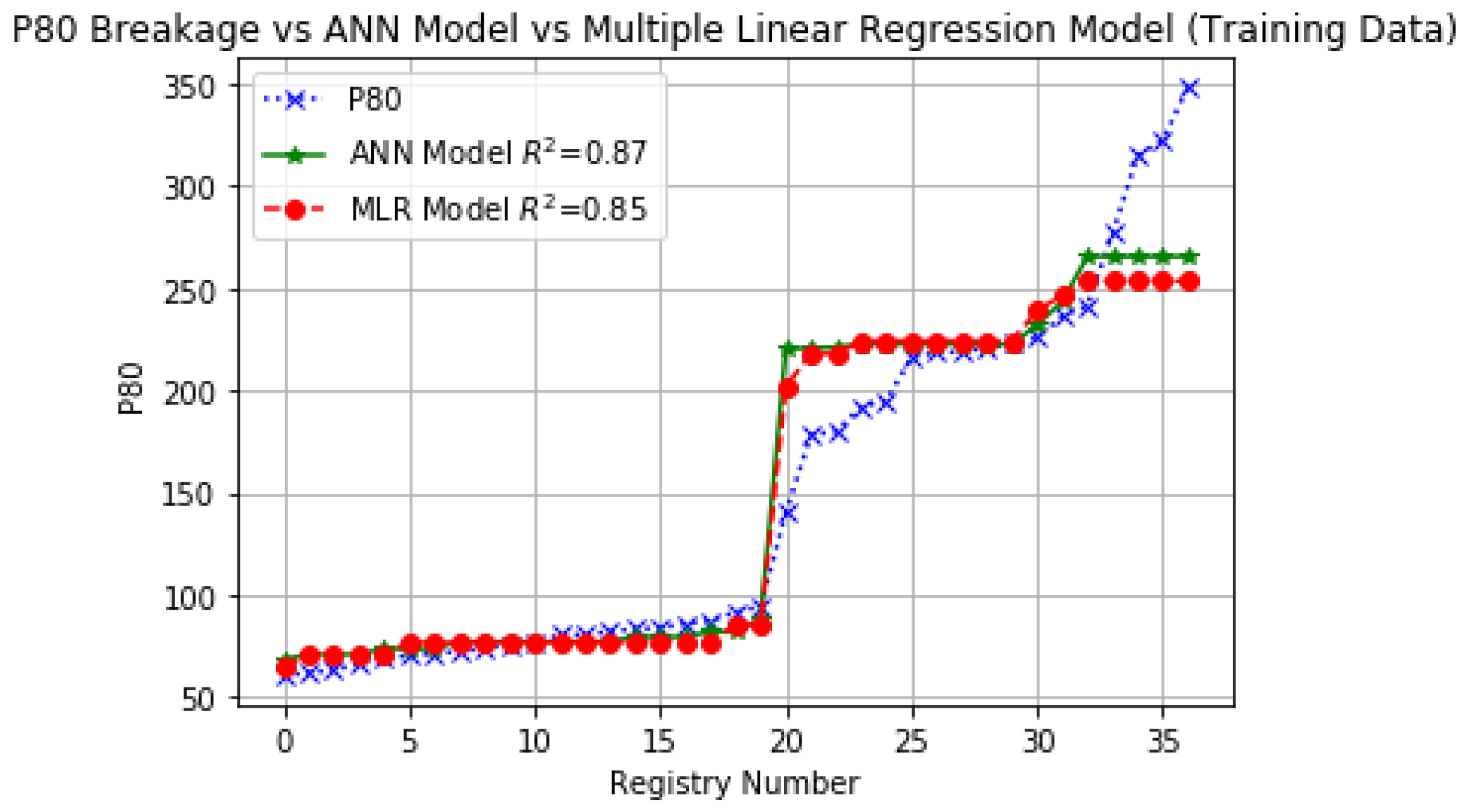
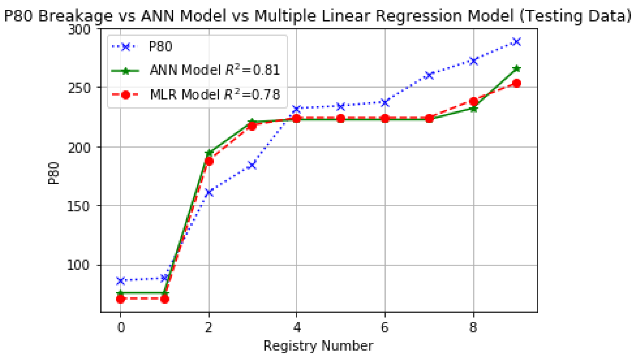
Figure 10 and
Figure 11 show a comparison among the ANN and MLR models of which, the ANN model depicts the greatest correlation according to
and
in training and testing respectively, as well as the other statistical parameters of the ANN model take values close to the real
according to
Table 3.
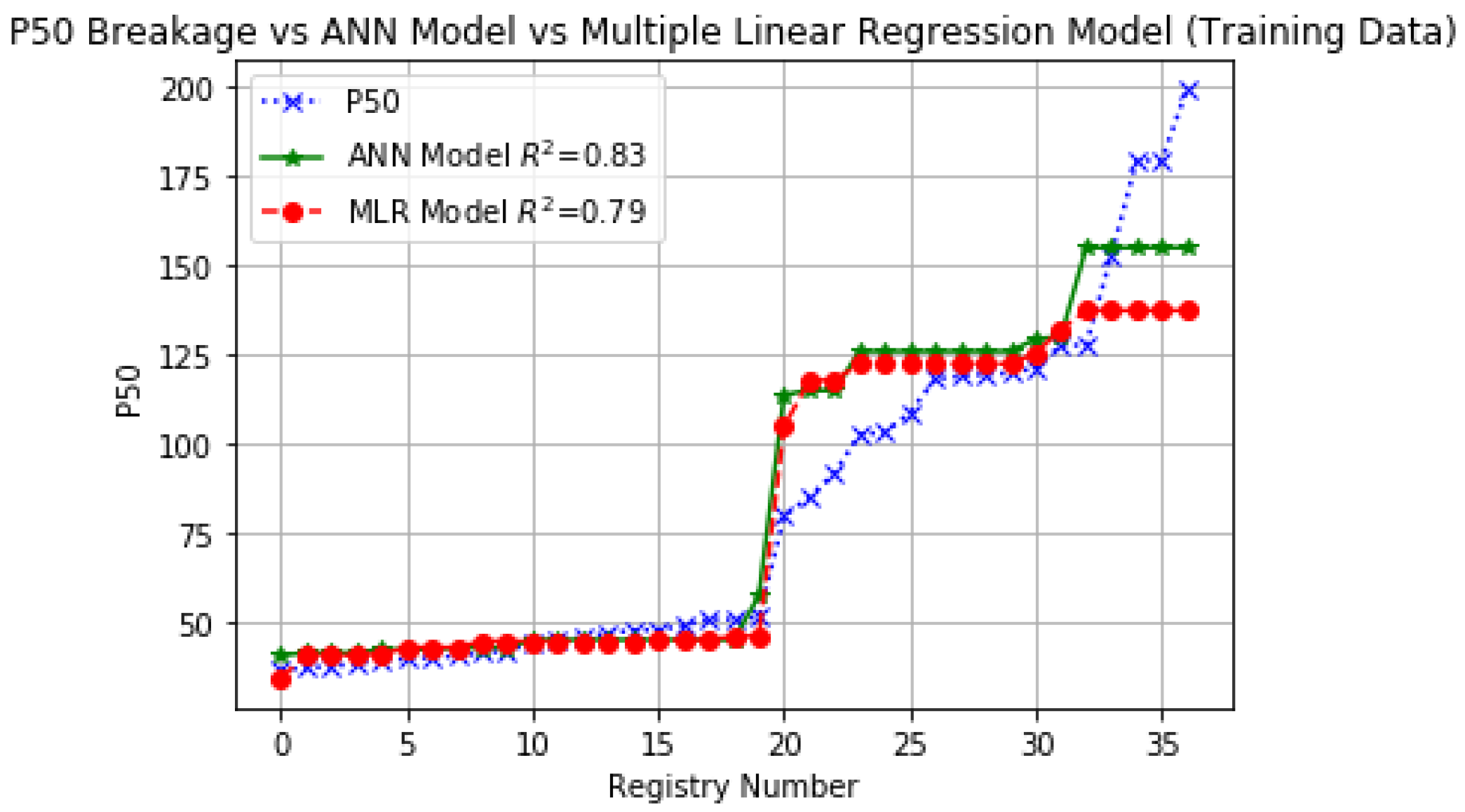
Figure 12 and
Figure 13 show a comparison among ANN and MLR models of which the ANN model depicts the greatest correlation according to
in training and other statistical parameters of the ANN model take values close to the real
according to
Table 4.
Figure 14 and
Figure 15 show a comparison of the ANN and MLR models of which the ANN model depicts the greatest correlation according to
in training, while in testing an
with similar values is shown, good results have been obtained for the prediction of
according to
Table 5.
The values obtained from the correlation coefficient of each studied ANN model (, and ) are quite acceptable and the breakage can be controlled in such a way that performance and costs can be improved in the subsequent mining processes such as: loading, hauling, crushing and grinding.
Although the ANN and MLR models have an acceptable degree of correlation, in the comparison curves, a marked difference is observed in the final fragmentation part of real , and with respect to the preceding values, this is due to the possibility of the absence of some input parameter that has been omitted in the data collection, which remains a future work, in which it is recommended to increase the number of input parameters to obtain an even more accurate model.
7. Conclusions
On the basis of the results obtained from this study, we observe that using the proposed ANN model, we get an increasing of coefficient of correlation () from 2% to 4 % over MRL in the comparisons made with the training data, while this percentage increase varies from 0% to 2% with the testing data over MRL, which is mainly due to the sample size. In addition, it is observed that the correlation coefficients in the training models decrease in the comparisons of , and ( = 0.87, 0.83 and 0.82). This is due to the fact that the main input variables are focused on the target of , and they decrease the effect on the variables and .
Therefore, the model obtained is an alternative to the one presented in the paper [
29], and shows moderately reliable results. However, it is important to continue monitoring the blasting records to feed the site database and ensure greater representativeness of the parameters in order to that the model has a greater extended further than in its predictions, especially if working with various types of mines with other peculiarities.
In the present study, we considered several training algorithms according to [
27]. In order to evaluate performance, the Momentum algorithm was selected because it reaches the global minimum and a marked stability in the root mean square error before the other algorithms.
Concerning to the linear models of the different variables , and it is concluded that their results have a moderate linear adjustment, but it tends to decrease in accuracy when the data testing has a well-marked dispersion. However, the ANN model “learned from the data” to obtain a variability very similar to the real data under study.
In future study we hope to use the ANN model with other real data from different mines, verifying the prediction efficiency and evaluating their associated costs.

 ,
, 


