An Efficient Numerical Scheme for Variable-Order Fractional Sub-Diffusion Equation

Abstract

The variable-order (VO) fractional calculus can be seen as a natural extension of the constant-order, which can be utilized in physical and biological applications. In this study, we derive a new numerical approximation for the VO fractional Riemann–Liouville integral formula and developed an implicit difference scheme (IDS) for the variable-order fractional sub-diffusion equation (VO-FSDE). The derived approximation used in the VO time fractional derivative with the central difference approximation for the space derivative. Investigated the unconditional stability by the van Neumann method, consistency, and convergence analysis of the proposed scheme. Finally, a numerical example is presented to verify the theoretical analysis and effectiveness of the proposed scheme.

1. Introduction

Fractional differential equations (FDEs) got the researchers attention and this fact states the phenomena in various areas such as biochemistry, wave propagation, medicine, anomalous diffusion, and electrical engineering, etc. [1,2,3,4]. The fractional diffusion equation is an important FDE, which has been hugely used in fractional diffusive systems, diffusion in transport processes, unification of diffusion phenomena and fractional random walk [5,6]. The fractional sub-diffusion equation (FSDE) is a subclass of the fractional diffusion equation and obtained by replacing the time derivative by fractional-order $\alpha$ lying between 0 and 1. The one-dimensional FSDE can be written as:

$$\begin{array}{c}\hfill \frac{\partial u(x,t)}{\partial t}=\frac{{\partial }^{1-\alpha }}{\partial t^{1-\alpha }}\left[\frac{{\partial }^{2}u(x,t)}{\partial x^2}\right]+f(x,t).\end{array}$$

(1)

where $\frac{{\partial }^{1-\alpha }}{\partial t^{1-\alpha }}$ represent the Riemann-Liouville fractional derivative (RL-FD) of order $1-\alpha$.

Most of the FDEs are not easy even impossible to get an analytical solution, which contains complicated functions. Therefore, numerical methods have become the main way for the solution of such types of fractional order differential equations. Many researchers have constructed the various numerical methods to solve FDEs such as Yuste [7] considered the weighted average implicit difference scheme (IDS) for the solution of FSDE. They discussed the theoretical analysis by the well known Fourier series method. Ali et al. [8] constructed a new numerical scheme for the modified FSDE. They investigated the theoretical analysis and found that the scheme is unconditionally stable and highly accurate. In another survey Ali et al. [9] derived a new approximation for RL-FD and developed compact IDS for modified FSDE. They successfully discussed the theoretical analysis and accuracy. Mohebbi et al. [10] studied the compact order IDS and solved the modified FSDE. They approximated the fractional derivative by Grünwald–Letnikov and the space derivative by fourth order approximation. The theoretical analysis are discussed by Fourier method and the tested examples shown high accuracy. Zhuang et al. [11] formulated the physical-mathematical method for FSDE and investigated a new numerical scheme. They analyzed the theoretical analysis based on energy method and the numerical values fully support the theoretical analysis. Ali et al. [12] proposed the Crank–Nicolson method for 2D-FSDE. They replaced the fractional derivative with Grünwald–Letnikov approximation and the space derivatives with finite difference approximation. They discussed the theoretical analysis with unconditional stability and convergence. Khan and Rasheed [13] studied the mixed convection in an incompressible fractional Maxwell nanofluid with thermal transmission. They tackled the arising mathematical problem numerically via finite difference procedure in their reported study they have mentioned that escalating values of Prandtl number reduces the thermal transport. Hamid et al. [14] investigated the modeling of unsteady radiating fractional nanofluid problem in a channel. Fractional derivative in Caputo sense is engaged in the model problem. They computed the solution of the boundary layer equations with the help of Crank–Nicolson numerical scheme. They found that the magnetic parameter reduces the velocity, whereas, Grashof number boosts fluid velocity. Other related literature can be seen in [15,16,17,18]. The above cited studies are reported the fractional derivative of constant-order.

The constant-order fractional derivatives are sometimes not more suitable to explain the complex diffusion processes as in porous medium and medium structure because it changes with time [19,20]. In VO operator the order may vary as function of independent variables such as time or space or both time-space. Lorenzo and Hartly [21] discussed some physical phenomena which show that the fractional-order behavior may change with time and space. To solve such type of VO fractional model and developed some numerical techniques. Here, we include only the VO-FSDE, which can be written as:

$$\begin{array}{c}\hfill \frac{\partial u(x,t)}{\partial t}=\frac{{\partial }^{1-\alpha (x,t)}}{\partial t^{1-\alpha (x,t)}}\left[\frac{{\partial }^{2}u(x,t)}{\partial x^2}\right]+f(x,t).\end{array}$$

(2)

There are many researchers who have worked on a VO-FSDE and find the solution by different numerical techniques such as Chen et al [22] developed a numerical scheme for VO-FSDE with first-order temporal and fourth-order spatial accuracy. they investigated the stability, convergence, and solvability analysis by Fourier series method. Lin et al [23] consider the nonlinear VO-FSDE and construct a new numerical finite difference scheme, also discussed stability and convergence analysis. Sun et al. [24] discussed different complex diffusion processes that can be described by the VO model. They differentiate this model into four types such as time-dependent, space-dependent, concentration-dependent, and system parameter dependent models. Sweilam et al. [25] solved the VO Riesz space fractional wave equation by explicit difference method. They discussed the Riesz space fractional derivatives based on shifted Grünwald–Letnikov formula and also established the stability and convergence analysis. Chen et al. [26] formulated the numerical solution for the nonlinear VO-FSDE. They proposed the piecewise function for VOFD and then by operational matrices transformed into an algebraic equation. Bhrawy and Zaky [27] investigated a numerical method based on the collocation method combined with Jacobi operational matrix and successfully solved the one and 2D-VO fractional Cable equations. They analyzed the convergence analysis and the numerical results demonstrated that the algorithm is powerful with high accuracy. Chen [28] solved the 2D-VO modified FSDE by numerical method. They discussed the stability, convergence, and solvability by the Fourier method. The two new second order numerical approximations are derived for VO time-fractional operator by Zhao et al. [29]. They tested on VO-FSDE and super-diffusion problems, the results are different than standard diffusion and constant-order diffusion for the VO $\alpha (x,t)$. Wang et al. [30] considered the VO-FDE with variable coefficient. They solved the problem by finite difference method and homotopy regularization method based on Legendre polynomials as the basis functions of approximation space. Ma et al. [31] discussed the numerical Adams-Bashforth-Moulton method for the VO fractional financial system of equations. The tested examples reported that the proposed method for VO-FDE is simple and effective. Shekari et al. [32] considered the moving least squares method to find the solution of 2D VO fractional diffusion-wave equation. They utilized the mesh free and collocation method based on moving least square approximation. Xu et al. [33] solved the multi-term VO space-time fractional diffusion equation on a finite domain by numerical method. Investigated the theoretical analysis via mathematical induction and numerical examples confirmed the efficiency and accuracy. Shen et al. [34] considered the Coimbra VO time derivative which is a Caputo type definition and used in the numerical scheme for variable -order fractional diffusion equation. The theoretical analyses are discussed by the well know Fourier series. Further, other related studies of fractional and VO-FDE can see in [35,36,37,38,39,40].

In this article, we developed a new implicit difference method to solve the VO-FSDE by applying the new discretized approximation for VO-RL fractional integral. The first order time derivative is replaced by backward difference approximation. Further, investigated the stability analysis by van Neumann method, consistency and convergence of the proposed method. The proposed scheme is very easy to implement, it decreases the computational complexity and increase efficiency. Another positive point of this scheme is, the easiness in finding the stability and convergence analysis.

This investigation is arranged as follows: Section 1, contains the comprehensive literature survey relevant to the reported material. In Section 2, briefly explain the mathematical preliminaries, we discussed the implicit scheme in Section 3. In Section 3.1 and Section 3.2, we use the van Neumann method to prove the stability and consistency respectively. In Section 4, provided the numerical experiments to confirm the theoretical analysis and in the last section concluded the conclusion.

2. Mathematical Preliminaries

In this section, we discuss the VO fractional calculus [41] and deriving new approximation for VO-RL fractional integral, which is used in this paper:

Definition 1.

The VO RL-FD formula can be written as:

$$\begin{array}{c}\hfill {}_0^{RL}{D}_t^{1-\alpha (x,t)}u(x,t)=\frac{1}{\mathsf{\Gamma }\left(\alpha \right(x,t\left)\right)}\frac{\partial }{\partial t}{\int }_0^t\frac{u(x,\eta )}{{(t-\eta )}^{1-\alpha (x,t)}}d\eta .\end{array}$$

(3)

Definition 2.

The VO-RL fractional integral formula can be written as:

$$\begin{array}{c}\hfill I_0^{\alpha (x,t)}u(x,t)=\frac{1}{\mathsf{\Gamma }\alpha (x,t)}{\int }_0^t\frac{u(x,\eta )}{{(t-\eta )}^{1-\alpha (x,t)}}d\eta .\end{array}$$

(4)

Here, we formulate a new numerical approximation for VO-RL fractional integral of order $\alpha (x,t)$ and $(0<\alpha (x,t)<1)$ at the grid point $(x_i,t_k)$, as following:

$$\begin{array}{cc}{I}_0^{\alpha (x_i,t_k)}u(x_i,t_k)=\hfill & \frac{1}{\mathsf{\Gamma }\alpha (x_i,t_k)}{\int }_0^{t_k}\frac{u(x_i,\xi )}{{(t_k-\xi )}^{1-\alpha (x_i,t_k)}}d\xi ,\hfill \\ \hfill & =\frac{1}{\mathsf{\Gamma }\alpha (x_i,t_k)}{\int }_0^{t_k}{(t_k-\xi )}^{\alpha (x_i,t_k)-1}u(x_i,\xi )d\xi ,\hfill \\ \hfill & ={\displaystyle \sum _{j=0}^{k-1}}{\int }_{t_j}^{t_{j+1}}\frac{{(t_k-\xi )}^{\alpha (x_i,t_k)-1}u(x_i,\xi )}{\mathsf{\Gamma }\alpha (x_i,t_k)}d\xi ,\hfill \\ \hfill & ={\displaystyle \sum _{j=0}^{k-1}}\frac{u(x_i,t_{k-j})}{\mathsf{\Gamma }\alpha (x_i,t_k)}{\int }_{t_j}^{t_{j+1}}{(t_k-\xi )}^{\alpha (x_i,t_k)-1}d\xi ,\hfill \\ \hfill & ={\displaystyle \sum _{j=0}^{k-1}}\frac{u(x_i,t_{k-j})}{\mathsf{\Gamma }\alpha (x_i,t_k)}\left(-\frac{{(t_k-\xi )}^{\alpha (x_i,t_k)}}{\alpha (x_i,t_k)}{|}_{t_j}^{t_{j+1}}\right),\hfill \\ \hfill & ={\displaystyle \sum _{j=0}^{k-1}}\frac{{\tau }^{\alpha (x_i,t_k)}u(x_i,t_{k-j})}{\mathsf{\Gamma }(1+\alpha (x_i,t_k))}\left({(j+1)}^{\alpha (x_i,t_k)}-{\left(j\right)}^{\alpha (x_i,t_k)}\right),\hfill \\ \hfill & ={\displaystyle \sum _{j=0}^{k-1}}\frac{{\tau }^{\alpha (x_i,t_k)}}{\mathsf{\Gamma }(1+\alpha (x_i,t_k))}({(j+1)}^{\alpha (x_i,t_k)}-{\left(j\right)}^{\alpha (x_i,t_k)})u(x_i,t_{k-j}).\hfill \end{array}$$

(5)

Lemma 1.

The VO $\alpha (x,t)(0<\alpha (x,t)<1)$ fractional RL integral of the function $u(x,t)$ on $[0,t]$ can be defined in discretized form at the grid point $(x_i,t_k)$ as:

$$I_0^{\alpha (x_i,t_k)}u(x_i,t_k)=C_i^k\sum _{j=0}^{k-1}{b}_j^{\left({\alpha }_i^k\right)}{u}_i^{k-j},$$

(6)

where $C_i^k=\frac{{\tau }^{{\alpha }_i^k}}{\mathsf{\Gamma }(1+{\alpha }_i^k)}$, $b_j=({(j+1)}^{{\alpha }_i^k}-{\left(j\right)}^{{\alpha }_i^k}).$

Lemma 2.

The coefficients $b_j^{\left({\alpha }_i^k\right)}(j=0,1,2,\dots )$ satisfy the following properties [39]:

(i) 

$b_0^{\left({\alpha }_i^k\right)}=1,b_j^{\left({\alpha }_i^k\right)}>0,j=0,1,2,\dots .$

(ii) 

$b_{j-1}^{\left({\alpha }_i^k\right)}>b_j^{\left({\alpha }_i^k\right)},j=1,2,\dots .$

(iii) 

There exists a positive constant $C>0,$ such that $\tau \le C{b}_j^{\left({\alpha }_i^k\right)}{\tau }^{{\alpha }_i^k},j=1,2,\dots .$

(iv) 

${\sum }_{j=0}^k{b}_j^{\left({\alpha }_i^k\right)}{\tau }^{{\alpha }_i^k}={(k+1)}^{{\alpha }_i^k}\le T^{{\alpha }_i^k}.$

3. The Implicit Scheme

To construct an IDS for VO-FSDE (2), first we use Equation (4), then applying lemma 1 for the discretization of RL fractional integral and for space derivative utilizing the central difference approximation. Here, the x variable steps as $x_i=i\mathsf{\Delta }x$, in the x-direction with $i=1,\dots ,M-1$, $\mathsf{\Delta }x=\frac{L}{M}$ and for t variable the step is $t_k=k\tau$,$k=1,\dots ,N$ where $\tau =\frac{T}{N}$. Let $u_i^k$ be the numerical approximation to $u(x_i,t_k)$, put Equation (4) into Equation (2), we have

$$\begin{array}{c}\hfill \frac{\partial u(x_i,t_k)}{\partial t}=\frac{\partial }{\partial t}{I}_0^{\alpha (x_i,t_k)}\frac{{\partial }^{2}u(x_i,t_k)}{\partial x^2}+f(x_i,t_k),\end{array}$$

(7)

by applying lemma 1 and backward difference approximation to Equation (7), we get

$$\begin{array}{c}\hfill u_i^k-u_i^{k-1}=\frac{{\tau }^{{\alpha }_i^k}}{{\left(\mathsf{\Delta }x\right)}^2\mathsf{\Gamma }(1+{\alpha }_i^k)}\sum _{j=0}^{k-1}{b}_j^{\left({\alpha }_i^k\right)}{\delta }_x^2(u_i^{k-j}-u_i^{k-j-1})+\tau f_i^k.\end{array}$$

(8)

Simplifying Equation (8), we get a new IDS for the one-dimensional VO-FSDE (2) with the conditions, as follows

$$\begin{array}{ll}-C_i^k{u}_{i+1}^k+(1+2C_i^k)u_i^k-C_i^k{u}_{i-1}^k=u_i^{k-1}-\hfill & C_i^k{b}_{k-1}^{\left({\alpha }_i^k\right)}(u_{i+1}^0-2u_i^0+u_{i-1}^0)+\hfill \\ \hfill & C_i^k{\displaystyle \sum _{j=1}^{k-1}}(b_j^{\left({\alpha }_i^k\right)}-b_{j-1}^{\left({\alpha }_i^k\right)})(u_{i+1}^{k-j}-2u_i^{k-j}+u_{i-1}^{k-j})+\tau f_i^k.\hfill \end{array}$$

(9)

Here,

$$\begin{array}{c}{C}_j=\frac{{\tau }^{{\alpha }_i^k}}{{\left(\mathsf{\Delta }x\right)}^2\mathsf{\Gamma }(1+{\alpha }_i^k)},{\delta }_x^2{u}_i^k=u_{i+1}^k-2u_i^k+u_{i-1}^k,\end{array}$$

(10)

and $i=1,2,\dots ,M_x-1$, and $k=1,2,\dots ,N-1,$ with

$$u_i^0=\phi \left(x_i\right),$$

(11)

$$\begin{array}{c}\hfill u_0^k={\phi }_1\left(t_k\right),u_{M,}^k={\phi }_2\left(t_k\right),0\le x\le L,0\le t\le T.\end{array}$$

(12)

3.1. Stability

To analyze the stability of the proposed IDS using van Neumann method. Let $U_i^k$ represent the approximated solution for (9), we obtained

$$\begin{array}{ll}-C_i^k{U}_{i+1}^k+(1+2C_i^k)U_i^k-C_i^k{U}_{i-1}^k=\hfill & U_i^{k-1}-C_i^k{b}_{k-1}^{\left({\alpha }_i^k\right)}(U_{i+1}^0-2U_i^0+U_{i-1}^0)+\hfill \\ \hfill & C_i^k\sum _{j=1}^{k-1}(b_j^{\left({\alpha }_i^k\right)}-b_{j-1}^{\left({\alpha }_i^k\right)})(U_{i+1}^{k-j}-2U_i^{k-j}+U_{i-1}^{k-j})+\tau f_i^k.\hfill \end{array}$$

(13)

The error is defined as

$$e_i^k=u_i^k-U_i^k,$$

(14)

where $e_i^k$ satisfies Equation (13), as

$$\begin{array}{ll}-C_i^k{e}_{i+1}^k+(1+2C_i^k)e_i^k-C_i^k{e}_{i-1}^k=e_i^{k-1}\hfill & -C_i^k{b}_{k-1}^{\left({\alpha }_i^k\right)}(e_{i+1}^0-2e_i^0+e_{i-1}^0)+\hfill \\ \hfill & C_i^k{\displaystyle \sum _{j=1}^{k-1}}(b_j^{\left({\alpha }_i^k\right)}-b_{j-1}^{\left({\alpha }_i^k\right)})(e_{i+1}^{k-j}-2e_i^{k-j}+e_{i-1}^{k-j}).\hfill \end{array}$$

(15)

The error initial and boundary conditions are given by

$$e_0^k=e_M^k=e_i^0=0.$$

(16)

By defining the following grid functions for $k=1,2,\dots ,N.$

$$e^k\left(x\right)=\left\{\begin{array}{c}{e}_i^k,when{x}_{i-\frac{\mathsf{\Delta }x}{2}}<x\le x_{i+\frac{\mathsf{\Delta }x}{2}},\hfill \\ 0,when0\le x\le \frac{\mathsf{\Delta }x}{2}orL-\frac{\mathsf{\Delta }x}{2}\le x\le L,\hfill \end{array}\right.$$

(17)

then $e^k\left(x\right)$ can be expanded in Fourier series such as:

$$e^k\left(x\right)=\sum _{l_1=-\infty }^{\infty }{\lambda }^k\left(l_1\right)e^{2\sqrt{-1}\pi (l_{1}x/L)},$$

(18)

where

$${\lambda }^k\left(l_1\right)=\frac{1}{L}{\int }_0^L{\int }_0^L{e}^k\left(x\right)e^{-2\sqrt{-1}\pi (l_{1}x/L)}dx.$$

(19)

From the definition of $l^2$ norm and Parseval equality, we have

$$\Vert e^k{\Vert }_{\infty }^2=\sum _{i=1}^{M_x-1}\mathsf{\Delta }x|e_i^k{|}^2=\sum _{l_1}^{\infty }{\left|{\lambda }^k\left(l_1\right)\right|}^2.$$

(20)

Supposing that

$$e_i^k={\lambda }^k{e}^{\sqrt{-1}\left({\sigma }_{1}i\mathsf{\Delta }x\right)},$$

(21)

here, ${\sigma }_1=2\pi l_1/L$ and substituting (21) in (15), we obtain

$$\begin{array}{c}\hfill {\lambda }^k=\frac{1}{(1+{\mu }_i^k)}\left({\lambda }^{k-1}+{\mu }_i^k{b}_{k-1}^{\left({\alpha }_i^k\right)}{\lambda }^0-{\mu }_i^k\sum _{j=1}^{k-1}(b_{j-1}^{\left({\alpha }_i^k\right)}-b_j^{\left({\alpha }_i^k\right)}){\lambda }^{k-j}\right),\end{array}$$

(22)

where

$$\begin{array}{c}\hfill {\mu }_i^k=4C_i^{k}si{n}^2(\frac{{\sigma }_1\mathsf{\Delta }x}{2}).\end{array}$$

Proposition 1.

If ${\lambda }^k$$(k=1,2,\dots ,N)$ satisfy (22), then $|{\lambda }^k|\le |{\lambda }^0|.$

Proof. 

By using mathematical induction, we take $k=1$ in (22)

$${\lambda }^1=\frac{(1+{\mu }_i^1{b}_0^{\left({\alpha }_i^1\right)}){\lambda }^0}{(1+{\mu }_i^1)},$$

and as ${\mu }_i^1\ge 0$ and $b_0^{\left({\alpha }_i^1\right)}=1$, then

$$|{\lambda }^1|\le |{\lambda }^0|.$$

Now, assuming that

$$|{\lambda }^m|\le |{\lambda }^0|;m=1,2,\dots ,k-1.$$

As $0<{\alpha }_i^k<1$, from (22) and lemma 1, we have

$$\begin{array}{cc}|{\lambda }^k|\le \hfill & \frac{|{\lambda }^{k-1}|+{\mu }_i^k{b}_{k-1}^{\left({\alpha }_i^k\right)}|{\lambda }^0|+{\mu }_i^k{\sum }_{j=1}^{k-1}(b_{j-1}^{\left({\alpha }_i^k\right)}-b_j^{\left({\alpha }_i^k\right)})|{\lambda }^{k-j}|}{(1+{\mu }_i^k)},\hfill \\ \hfill & \le \left[\frac{1+{\mu }_i^k{b}_{k-1}^{\left({\alpha }_i^k\right)}+{\mu }_i^k{\sum }_{j=1}^{k-1}(b_{j-1}^{\left({\alpha }_i^k\right)}-b_j^{\left({\alpha }_i^k\right)})}{(1+{\mu }_i^k)}\right]\left|{\lambda }^0\right|,\hfill \\ \hfill & =\left[\frac{1+{\mu }_i^k{b}_{k-1}^{\left({\alpha }_i^k\right)}+{\mu }_i^k(b_0^{\left({\alpha }_i^1\right)}-b_{k-1}^{\left({\alpha }_i^k\right)})}{(1+{\mu }_i^k)}\right]\left|{\lambda }^0\right|,\hfill \\ \hfill & =\left[\frac{1+{\mu }_i^k}{1+{\mu }_i^k}\right]\left|{\lambda }^0\right|,\hfill \\ & |{\lambda }^k|\le |{\lambda }^0|.\hfill \end{array}$$

(23)

From the above proof, it is clear that Proposition 1 and Equation (20), reported that the solution of Equation (9) satisfies

$$\Vert {\lambda }^k{\Vert }_2\le {\Vert {\lambda }^0\Vert }_2,$$

this proved that the IDS in (9) is unconditionally stable. ☐

3.2. Consistency

To analyse the consistency of the IDS, let U be the exact and u be the approximate solution and $F\left(U\right)=0$ represent the approximated difference equation of the FDE (2) at point $(x_i,t_k)$, then $F\left(u\right)=T_i^k$ represented the truncation error at grid point $(x_i,t_k)$.

Theorem 1.

The truncation error $T(x,t)$ of the proposed difference scheme is: $T_i^k=O\left(\mathsf{\Delta }t\right)+O\left(\mathsf{\Delta }{x}^2\right)$.

Proof. 

$$\begin{array}{c}\hfill T_i^k=u_i^k-u_i^{k-1}-C_i^k\sum _{j=0}^{k-1}{b}_j^{\left({\alpha }_i^k\right)}\left((u_{i+1}^{k-j}-2u_i^{k-j}+u_{i-1}^{k-j})-(u_{i+1}^{k-j-1}-2u_i^{k-j-1}+u_{i-1}^{k-j-1})\right).\end{array}$$

(24)

By Taylor expansion we can write

$$\begin{array}{cc}{T}_i^k=u_i^k-\hfill & \left(u_i^k-\left(\mathsf{\Delta }t\right)\frac{\partial u}{\partial t}{|}_i^k+\frac{{\left(\mathsf{\Delta }t\right)}^2}{2}\frac{{\partial }^{2}u}{\partial t^2}{|}_i^k+\dots \right)-\hfill \\ \hfill & C_i^k{\displaystyle \sum _{j=0}^{k-1}}{b}_j^{\left({\alpha }_i^k\right)}\left[\right(\left(u_i^k+\left(\mathsf{\Delta }x\right)\frac{\partial u}{\partial x}{|}_i^{k-j}+\frac{{\left(\mathsf{\Delta }x\right)}^2}{2}\frac{{\partial }^{2}u}{\partial x^2}{|}_i^{k-j}+\frac{{\left(\mathsf{\Delta }x\right)}^3}{6}\frac{\partial u^3}{\partial x^3}{|}_i^{k-j}+\dots \right)\hfill \\ \hfill & -2u_i^{k-j}+\left(u_i^k-\left(\mathsf{\Delta }x\right)\frac{\partial u}{\partial x}{|}_i^{k-j}+\frac{{\left(\mathsf{\Delta }x\right)}^2}{2}\frac{{\partial }^{2}u}{\partial x^2}{|}_i^{k-j}-\frac{{\left(\mathsf{\Delta }x\right)}^3}{6}\frac{{\partial }^{3}u}{\partial x^3}{|}_i^{k-j}+\dots \right)-\hfill \\ \hfill & (\left(u_i^{k-j-1}+\left(\mathsf{\Delta }x\right)\frac{\partial u}{\partial x}{|}_i^{k-j-1}+\frac{{\left(\mathsf{\Delta }x\right)}^2}{2}\frac{{\partial }^{2}u}{\partial x^2}{|}_i^{k-j-1}+\frac{{\left(\mathsf{\Delta }x\right)}^3}{6}\frac{{\partial }^{3}u}{\partial x^3}{|}_i^{k-j-1}+\dots \right)-\hfill \\ \hfill & \hfill 2u_i^{k-j-1}+\left(u_i^{k-j-1}-\left(\mathsf{\Delta }x\right)\frac{\partial u}{\partial x}{|}_i^{k-j-1}+\frac{{\left(\mathsf{\Delta }x\right)}^2}{2}\frac{{\partial }^{2}u}{\partial x^2}{|}_i^{k-j-1}-\frac{{\left(\mathsf{\Delta }x\right)}^3}{6}\frac{{\partial }^{3}u}{\partial x^3}{|}_i^{k-j-1}+\dots \right)\left)\right],\end{array}$$

and

$$\begin{array}{c}{T}_i^k=\left(-\left(\mathsf{\Delta }t\right)\frac{\partial u}{\partial t}{|}_i^k+\frac{{\left(\mathsf{\Delta }t\right)}^2}{2}\frac{{\partial }^{2}u}{\partial t^2}{|}_i^k+\dots \right)-\hfill \\ C_i^k{\displaystyle \sum _{j=0}^{k-1}}{b}_j^{\left({\alpha }_i^k\right)}[{\left(\mathsf{\Delta }x\right)}^2\left(\frac{{\partial }^{2}u}{\partial x^2}{|}_i^{k-j}-\frac{{\partial }^{2}u}{\partial x^2}{|}_i^{k-j-1}\right)\\ \hfill -\frac{{\left(\mathsf{\Delta }x\right)}^4}{12}\left(\frac{{\partial }^{4}u}{\partial x^2}{|}_i^{k-j}+\dots -\frac{{\partial }^{4}u}{\partial x^4}{|}_i^{k-j-1}+\dots \right)].\end{array}$$

After simplification, we get the following truncation error

$$\begin{array}{c}\hfill T_i^k=O\left(\mathsf{\Delta }t\right)+O{\left(\mathsf{\Delta }x\right)}^2.\end{array}$$

This theorem shows that the proposed scheme is consistent if $\mathsf{\Delta }x$→ 0 and $\mathsf{\Delta }t$→ 0, then the truncation error tends to zero. ☐

Theorem 2.

According to Lax equivalence theorem, consistency and stability are both necessary and sufficient for convergence [39], the proposed VO-IDS is convergent.

4. Numerical Experiments

The numerical example of VO-FSDE are presented in this section to confirm the effectiveness of the new IDS. Here, we compute the $E_{\infty }$ and $E_2$ norm error, is defined as follows:

$$\begin{array}{c}\hfill E_{\infty }=\underset{0\le i\le M_x-1,0\le k\le N}{max}|u(x_i,t_k)-u_i^k|,E_2={\left(\left(\mathsf{\Delta }x\right)\sum _{i=1}^{M_x-1}|u(x_i,t_k)-u_i^k|\right)}^{\frac{1}{2}}.\end{array}$$

(25)

Example 1.

Consider the VO-FSDE is as following [19]:

$$\begin{array}{c}\hfill \frac{\partial u(x,t)}{\partial t}=\frac{{\partial }^{1-\alpha (x,t)}}{\partial t^{1-\alpha (x,t)}}\left[\frac{{\partial }^{2}u(x,t)}{\partial x^2}\right]+2e^x\left(t-\frac{t^{1+\alpha (x,t)}}{\mathsf{\Gamma }(2+\alpha (x,t\left)\right)}\right),0\le t\le T,0<x<1,\end{array}$$

(26)

the initial and the boundary conditions are

$$\begin{array}{c}u(x,0)=0,0\le x\le 1,\\ u(0,t)=t^2,u(1,t)=e{t}^2,0\le x\le L,0\le t\le T.\hfill \end{array}$$

(27)

The exact solution is

$$u(x,t)=e^x{t}^2.$$

(28)

Table 1. Comparison of the implicit difference scheme (IDS) for different values of $\alpha (x,t)$ and at fixed values of $\mathsf{\Delta }x=\frac{1}{100}$, $T=1.0.$

	Error E∞		Error E2
	τ	[19]	Method	[19]	Method
$\alpha (x,t)=\frac{e^{-xt}}{400}$	$1/4$	6.0309$\times {10}^{-3}$	2.1024$\times {10}^{-4}$	4.4044$\times {10}^{-2}$	1.5379$\times {10}^{-4}$
	$1/8$	1.5166$\times {10}^{-3}$	6.2311$\times {10}^{-5}$	1.1078$\times {10}^{-2}$	4.3215$\times {10}^{-5}$
	$1/16$	3.7704$\times {10}^{-4}$	5.2566$\times {10}^{-5}$	2.7545$\times {10}^{-3}$	3.3345$\times {10}^{-5}$
	$1/32$	9.3918$\times {10}^{-5}$	1.1145$\times {10}^{-5}$	6.8622$\times {10}^{-4}$	7.7436$\times {10}^{-5}$
$\alpha (x,t)=\frac{2+sin\left(xt\right)}{400}$	$1/4$	6.0281$\times {10}^{-3}$	7.9047$\times {10}^{-4}$	4.4023$\times {10}^{-2}$	5.7621$\times {10}^{-4}$
	$1/8$	1.5171$\times {10}^{-3}$	5.7892$\times {10}^{-4}$	1.1081$\times {10}^{-2}$	4.2120$\times {10}^{-4}$
	$1/16$	3.7741$\times {10}^{-4}$	1.3667$\times {10}^{-4}$	2.7572$\times {10}^{-3}$	3.1659$\times {10}^{-4}$
	$1/32$	9.4057$\times {10}^{-5}$	3.4864$\times {10}^{-5}$	6.8721$\times {10}^{-4}$	2.5194$\times {10}^{-4}$
$\alpha (x,t)=\frac{2xt+1}{300}$	$1/4$	6.0318$\times {10}^{-3}$	8.1499$\times {10}^{-4}$	4.4051$\times {10}^{-2}$	5.9070$\times {10}^{-4}$
	$1/8$	1.5182$\times {10}^{-3}$	7.4512$\times {10}^{-4}$	1.1089$\times {10}^{-2}$	5.3748$\times {10}^{-4}$
	$1/16$	3.7704$\times {10}^{-4}$	5.2566$\times {10}^{-5}$	2.7545$\times {10}^{-3}$	3.3345$\times {10}^{-5}$
	$1/32$	9.4079$\times {10}^{-5}$	4.5761$\times {10}^{-5}$	6.8736$\times {10}^{-4}$	2.7098$\times {10}^{-5}$

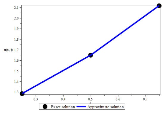
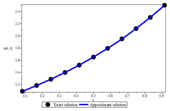
and

Table 2. The numerical results for Equation (26) at $T=1.0$.

$\mathit{\alpha }(\mathit{x},\mathit{t})$	$\mathit{\tau }=\mathbf{\Delta }\mathit{x}=10$	$\mathit{\tau }=\mathbf{\Delta }\mathit{x}=20$	$\mathit{\tau }=\mathbf{\Delta }\mathit{x}=40$	$\mathit{\tau }=\mathbf{\Delta }\mathit{x}=80$
$\frac{2cos\left(xt\right)+\left(xt\right)}{56}$	2.6785$\times {10}^{-3}$	1.5233$\times {10}^{-3}$	8.6046$\times {10}^{-4}$	6.1524$\times {10}^{-4}$
$\frac{1-{\left(xt\right)}^3+co{s}^2\left(xt\right)}{10}$	2.2091$\times {10}^{-3}$	1.4258$\times {10}^{-3}$	8.4040$\times {10}^{-4}$	4.3821$\times {10}^{-4}$
$\frac{30+{\left(xt\right)}^4}{750}$	2.0303$\times {10}^{-3}$	1.1525$\times {10}^{-3}$	6.5034$\times {10}^{-4}$	3.6267$\times {10}^{-4}$
$\frac{15+{\left(sin\left(xt\right)\right)}^8}{400}$	1.9153$\times {10}^{-3}$	1.0868$\times {10}^{-3}$	6.1368$\times {10}^{-4}$	2.8031$\times {10}^{-4}$
$\frac{10-{\left(xt\right)}^4}{300}$	1.7106$\times {10}^{-3}$	9.5885$\times {10}^{-4}$	5.3223$\times {10}^{-4}$	2.9679$\times {10}^{-4}$
$\frac{2+sin\left(xt\right)}{400}$	5.3892$\times {10}^{-4}$	4.3962$\times {10}^{-4}$	1.4306$\times {10}^{-4}$	7.7335$\times {10}^{-5}$
$\frac{2^{\left(xt\right)}-sin\left(xt\right)}{50}$	8.9348$\times {10}^{-4}$	3.8637$\times {10}^{-4}$	1.0794$\times {10}^{-4}$	5.7894$\times {10}^{-5}$

shows the numerical results of the new VO IDS for Equation (26). In Figure 1, the numerical values are compared with the previous study in Cao et al. [19] for various values of time steps and fixed space step. The proposed VO scheme reported better level of accuracy and more efficiency. Table 2 show that the error is reduced as the number of space and time steps increased. Figure 1 and Figure 2 are plotted for numerical scheme and compared it with exact solution for different values of $\alpha (x,t)=\frac{2^{-xt}-sin\left(xt\right)}{50},\frac{2+sin\left(xt\right)}{400}$, and $y=0.25,0.083$ and $T=1.0$ respectively. The above discussion proved that new IDS for VO-FDEs is accurate and numerically more efficient.

5. Conclusions

In this article, first we derived a new approximation for VO-RL fractional integral and for space derivative used the implicit central difference approximation. Successfully utilized the new numerical approximation and the IDS for one-dimensional VO-FSDE. Investigated the theoretical analysis by the well-known von Neumann method. The scheme is unconditionally stable and convergent with order $O(\tau +{\left(\mathsf{\Delta }x\right)}^2)$. The tested example result has compared with the previous study and with the exact solution for various values of $\alpha (x,t)$. We concluded that the scheme is a more effective, high level of accuracy and the solution is well-matched. We believe that this finding is another contribution to the literature. This numerical approximation can also be applied to other types of variable-order fractional differential equations.

References

- Li, X.; Wong, P.J. A new implicit numerical scheme for fractional sub-diffusion equation. In Proceedings of the 2016 14th International Conference on Control, Automation, Robotics and Vision (ICARCV), Phuket, Thailand, 13–15 November 2016; pp. 1–6. [Google Scholar]
- Zhang, P.; Pu, H. A second-order compact difference scheme for the fourth-order fractional sub-diffusion equation. Numer. Algorithms 2017, 76, 573–598. [Google Scholar] [CrossRef]
- Oldham, K.B.; Spanier, J. Fractional Calculus; Academic Press: New York, NY, USA; London, UK, 1974. [Google Scholar]
- Podlubny, I. Fractional Differential Equations; Academic Press: New York, NY, USA, 1999. [Google Scholar]
- Zhang, J.; Ye, C. High order numerical method and its analysis of the anomalous subdiffusion equation. Procedia Eng. 2012, 31, 781–790. [Google Scholar] [CrossRef][Green Version]
- Zhang, Y.N.; Sun, Z.Z. Alternating direction implicit schemes for the two-dimensional fractional sub-diffusion equation. J. Comput. Phys. 2011, 230, 8713–8728. [Google Scholar] [CrossRef]
- Yuste, S.B. Weighted average finite difference methods for fractional diffusion equations. J. Comput. Phys. 2006, 216, 264–274. [Google Scholar] [CrossRef]
- Ali, U.; Abdullah, F.A.; Mohyud-Din, S.T. Modified implicit fractional difference scheme for 2D modified anomalous fractional sub-diffusion equation. Adv. Diff. Equ. 2017, 185, 1–14. [Google Scholar] [CrossRef]
- Ali, U.; Sohail, M.; Usman, M.; Abdullah, F.A.; Khan, I.; Nisar, K.S. Fourth-Order Difference Approximation for Time-Fractional Modified Sub-Diffusion Equation. Syemmetry 2010, 12, 691. [Google Scholar] [CrossRef]
- Mohebbi, A.; Abbaszadeh, M.; Dehghan, M. A high-order and unconditionally stable scheme for the modified anomalous fractional sub-diffusion equation with a nonlinear source term. J. Comp. Phys. 2013, 240, 36–48. [Google Scholar] [CrossRef]
- Zhuang, P.; Liu, F.; Anh, V.; Turne, I. New solution and analytical techniques of the implicit numerical methods for the anomalous sub-diffusion equation. SIAM J. Numer. Anal. 2008, 46, 1079–1095. [Google Scholar] [CrossRef]
- Ali, U.; Abdullah, F.A.; Ismail, A.I. Crank-Nicolson finite difference method for two-dimensional fractional sub-diffusion equation. J. Interpolat. Approx. Sci. Comput. 2017, 2017, 18–29. [Google Scholar] [CrossRef]
- Khan, A.Q.; Rasheed, A. Mixed convection magnetohydrodynamics flow of a nanofluid with heat transfer: A numerical study. Math. Probl. Eng. 2019, 2019, 8129564. [Google Scholar] [CrossRef]
- Hamid, M.; Zubair, T.; Usman, M.; Haq, R.U. Numerical investigation of fractional-order unsteady natural convective radiating flow of nanofluid in a vertical channel. AIMS Math. 2019, 4, 1416. [Google Scholar] [CrossRef]
- Ali, U.; Abdullah, F.A. Explicit Saul’yev finite difference approximation for two- dimensional fractional sub-diffusion equation. In Proceedings of the AIP Conference Proceedings, Pahang, Malaysia, 27–29 August 2018; Volume 1, p. 020111. [Google Scholar]
- Liangliang, M.A.; Dongbing, L. An implicit difference approximation for fractional cable equation in high-dimensional case. J. Liao. Tech. University (Nat. Sci.) 2014, 4, 024. [Google Scholar]
- Zhai, S.; Feng, X.; He, Y. An unconditionally stable compact ADI method for 3D time-fractional convection-diffusion equation. J. Comp. Phys. 2014, 269, 138–155. [Google Scholar] [CrossRef]
- Zhuang, P.; Liu, F.; Turner, L.; Anh, V. Galerkin finite element method and error analysis for the fractional cable equation. Numer. Algor. 2016, 72, 447–466. [Google Scholar] [CrossRef]
- Cao, J.; Qiu, Y.; Song, G. A compact finite difference scheme for variable order subdiffusion equation. Commun. Nonlinear Sci. Numer. Simul. 2017, 48, 140–149. [Google Scholar] [CrossRef]
- Sun, H.; Chen, W.; Li, C.; Chen, Y. Finite difference schemes for variable-order time fractional diffusion equation. Int. J. Bifurc. Chaos 2012, 22, 1250085. [Google Scholar] [CrossRef]
- Lorenzo, C.F.; Hartley, T.T. Variable order and distributed order fractional operators. Nonlinear Dyn. 2002, 29, 57–98. [Google Scholar] [CrossRef]
- Chen, C.M.; Liu, F.; Anh, V.; Turner, I. Numerical schemes with high spatial accuracy for a variable-order anomalous subdiffusion equation. SIAM J. Sci. Comput. 2010, 32, 1740–1760. [Google Scholar] [CrossRef]
- Lin, R.; Liu, F.; Anh, V.; Turner, I. Stability and convergence of a new explicit finite-difference approximation for the variable-order nonlinear fractional diffusion equation. Appl. Math. Comput. 2009, 212, 435–445. [Google Scholar] [CrossRef]
- Sun, H.; Chen, W.; Chen, Y. Variable-order fractional differential operators in anomalous diffusion modeling. Phy. A Stat. Mech. Its Appl. 2009, 388, 4586–4592. [Google Scholar] [CrossRef]
- Sweilam, N.; Khader, M.; Almarwm, H. Numerical studies for the variable-order nonlinear fractional wave equation. Fract. Calc. Appl. Anal. 2012, 15, 669–683. [Google Scholar] [CrossRef][Green Version]
- Chen, C.M.; Liu, F.; Turner, I.; Anh, V. Numerical methods with fourth-order spatial accuracy for variable-order nonlinear Stokes’ first problem for a heated generalized second grade fluid. Comput. Math. Appl. 2011, 62, 971–986. [Google Scholar] [CrossRef]
- Bhrawy, A.H.; Zaky, M.A. Numerical simulation for two-dimensional variable-order fractional nonlinear cable equation. Nonlinear Dyn. 2015, 80, 101–116. [Google Scholar] [CrossRef]
- Chen, C.M. Numerical methods for solving a two-dimensional variable-order modified diffusion equation. Appl. Math. Comput. 2013, 225, 62–78. [Google Scholar] [CrossRef]
- Zhao, X.; Sun, Z.Z.; Karniadakis, G.E. Second-order approximations for variable order fractional derivatives: Algorithms and applications. J. Comput. Phys. 2015, 293, 184–200. [Google Scholar] [CrossRef]
- Wang, S.; Wang, Z.; Li, G.; Wang, Y. A simultaneous inversion problem for the variable-order time fractional differential equation with variable coefficient. Math. Probl. Eng. 2019, 2019, 2562580. [Google Scholar] [CrossRef]
- Ma, S.; Xu, Y.; Yue, W. Numerical solutions of a variable-order fractional nancial system. J. Appl. Math. 2012, 2012, 417942. [Google Scholar] [CrossRef]
- Shekari, Y.; Tayebi, A.; Heydari, M.H. A meshfree approach for solving 2D variable-order fractional nonlinear diffusion-wave equation. Comput. Methods Appl. Mech. Eng. 2019, 350, 154–168. [Google Scholar] [CrossRef]
- Xu, T.; Lü, S.; Chen, W.; Chen, H. Finite difference scheme for multi-term variable-order fractional diffusion equation. Adv. Diff. Equ. 2018, 2018, 103. [Google Scholar] [CrossRef]
- Shen, S.; Liu, F.; Chen, J.; Turner, I.; Anh, V. Numerical techniques for the variable order time fractional diffusion equation. Appl. Math. Comput. 2012, 218, 10861–10870. [Google Scholar] [CrossRef]
- Ali, U.; Abdullah, F.A. Modified implicit difference method for one-dimensional fractional wave equation. In Proceedings of the AIP Conference Proceedings, Penang, Malaysia, 10–12 December 2019; Volume 2184, p. 0060021.
- Bhrawy, A.H.; Zaky, M. Numerical algorithm for the variable-order Caputo fractional functional differential equation. Nonlinear Dyn. 2016, 85, 1815–1823. [Google Scholar] [CrossRef]
- Chen, Y.M.; Wei, Y.Q.; Liu, D.Y.; Yu, H. Numerical solution for a class of nonlinear variable order fractional differential equations with Legendre wavelets. Appl. Math. Lett. 2015, 46, 83–88. [Google Scholar] [CrossRef]
- Yaghoobi, S.; Moghaddam, B.P.; Ivaz, K. An efficient cubic spline approximation for variable-order fractional differential equations with time delay. Nonlinear Dyn. 2017, 87, 815–826. [Google Scholar] [CrossRef]
- Ali, U. Numerical Solutions for Two Dimensional Time-Fractional Differential Sub-Diffusion Equation. Ph.D. Thesis, University Sains Malaysia, Penang, Malaysia, 2019; pp. 1–200. [Google Scholar]
- Samko, S.G. Fractional integration and differentiation of variable order. Anal. Math. 1995, 21, 213–236. [Google Scholar] [CrossRef]
- Samko, S.G.; Kilbas, A.A.; Marichev, O.I. Fractional Integrals and Derivaives, Theory and Applications; Gordon and Breach Science Publishers: New York, NY, USA, 1993. [Google Scholar]
© 2020 by the authors. Licensee MDPI, Basel, Switzerland. This article is an open access article distributed under the terms and conditions of the Creative Commons Attribution (CC BY) license (http://creativecommons.org/licenses/by/4.0/).