Abstract
The operational matrices-based computational algorithms are the promising tools to tackle the problems of non-integer derivatives and gained a substantial devotion among the scientific community. Here, an accurate and efficient computational scheme based on another new type of polynomial with the help of collocation method (CM) is presented for different nonlinear multi-order fractional differentials (NMOFDEs) and Bagley–Torvik (BT) equations. The methods are proposed utilizing some new operational matrices of derivatives using Chelyshkov polynomials (CPs) through Caputo’s sense. Two different ways are adopted to construct the approximated (AOM) and exact (EOM) operational matrices of derivatives for integer and non-integer orders and used to propose an algorithm. The understudy problems have been transformed to an equivalent nonlinear algebraic equations system and solved by means of collocation method. The proposed computational method is authenticated through convergence and error-bound analysis. The exactness and effectiveness of said method are shown on some fractional order physical problems. The attained outcomes are endorsing that the recommended method is really accurate, reliable and efficient and could be used as suitable tool to attain the solutions for a variety of the non-integer order differential equations arising in applied sciences.
1. Introduction
The subject of fractional calculus (FC) and fractional or non-integer differential equations (FDEs) is an inspirational mathematical topic of research among scientific community. In 1695, this antique area is carried out from a famous dialogue between two conspicuous mathematicians Hospital and Leibniz. Indeed, the FC area is an old topic as traditional calculus proposed individually by Leibniz and Newton, but FC gained a vital importance among the researcher community. The devotion of scientific communities is pretty realistic due to its specific appearance in mathematical as well as other areas of science and engineering [1]. However, it converts the symbolization of derivatives for those sections where the order of the derivatives is non-integer or fractional. Recently, the subject of FC has been developed in different domains of sciences, from pure mathematical theories to modeling fractional order physical problems in different disciplines of engineering and applied sciences including ultra-capacitor, beam heating, transfer of heat in heterogeneous media, etc. [2]. Physical and natural mechanisms can be modeled using the differential equations and the solution of integer and non-integer order problems are worthy to compute because it saves both time and money [3,4,5]. The main impact of using FDEs states the non-local properties, which means that the present state and all its earlier states impact the subsequent state of the dynamical systems. The mentioned practical situations are normally due to the fact that a number of physical structures are associated to non-integer order dynamics and their deeds are directed by fractional differential equations (FDEs). The readers are referred to see the cited references [1,6] to review some fundamental concepts of fractional calculus and its potential applications as well as various techniques to compute fractional or non-integer order integrals/derivatives. The fractional derivative of in Caputo’s sense [7] is used in this work and stated below in Equation (1).
The differential operator satisfies the properties in (2) where, and are the constants.
Many useful processes in engineering, applied and physical sciences can be effectively modeled by means of fractional order differential equations. A noticeable knowledge and analysis related potential application and theory of FC is cited in [8]. Recently, FC is arising in various disciplines of sciences including modeling of different fluid flow, mathematical biology, modeling of water waves, control and optimization theory, dynamical, advection-diffusion, electrical circuits, networking, etc. [9,10,11]. It is an imperative fact that the results of physical models based on FDEs are additionally complex compared with integer-order differential equations (DEs) or physical and engineering problems. The devotion of mathematical communities is to accomplish the mathematical modeling for a given physical system in terms of differential or integral equations and fetch a competent solution to deliver a hypothetical study that reaches to the similar level of experimental outcomes which makes the FDEs an emerging and hot research area in recent times.
To achieve this high level of accuracy and better analysis, various kinds of techniques including, analytical, numerical, soliton and wavelet have been adopted in the past [12,13,14,15,16,17,18,19,20,21]. Literature survey proved that there are many lacks to obtain the better approximation and analysis of fractional ordered problems arising in applied sciences. Recently, approximation through orthogonal basis functions has acknowledged more suitable and gained a substantial devotion in different areas of engineering and mathematical science. Indeed, algorithms depending upon the orthogonal basis functions converts the nonlinear problems under study to a set of linear or nonlinear algebraic equations and the obtained system could be solved to approximate the given problem. Previously, various kinds of polynomials including Bernstein, Chebyshev, Chelyshkov, Gegenbauer and shifted Gegenbauer, Jacobi, Laguerre, Laurent, Legendre and a few others had been utilized by researchers to examine different complex nature physical problems [22,23,24,25,26,27,28,29,30,31]. Lately, alternative kinds of orthogonal polynomials have been familiarized and adopted to evaluate the dynamics of the several types of problems governed by differential/integral equations. An algorithm based on operational matrices of integration using Chelyshkov polynomials is proposed by Mohammadi [32]. A Chelyshkov wavelet-based technique is developed to compute the control theory problems by Moradi et al. [33]. Readers are suggested to find some associated research to such polynomials in [34,35,36,37,38].
The motivation of the present work is to develop and compare some operational matrices of derivatives and use to propose a methodology to investigate the fractional order problems. The novel operational matrices are developed with the aid of a new kind of polynomial. The matrices are obtained by using two different approaches and later utilized to propose a computational algorithm together with collocation technique named Chelyshkov polynomial method (CPM). The CPM with exact operational matrix of derivative is termed as CPMEOM while CPM with approximate operational matrix is CPMAOM. The detailed evaluation is given in upcoming sections. The nonlinear fractional problems (multi-order and BT equations) under study have been investigated to show the reliability of the method. The BT-equation arises in FDE-NNs architecture and the flow chart is available in Figure 1 while a detailed description about the problem is given in Section 5. The outcomes have been compared with existing data in literature and exact solutions, whereas a set of graphical plots and a tabular comparison is presented. It is apparent that the developed computational scheme is an effectual tool and could be prolonged to evaluate the physical, dynamical and complex natured nonlinear non-integer order problems. More precisely, the method can be extended by coupling with other methods as well as for problem governed by integral equations.
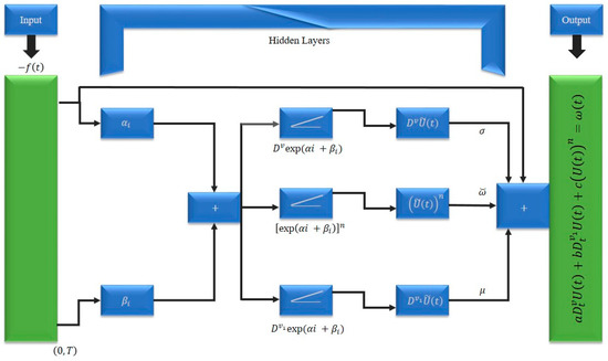
Figure 1.
The Bagley–Torvik (BT) equation arise in FDE-NNs architecture.
2. Chelyshkov Polynomials
Herein, we will determine the basic definition of Chelyshkov polynomial as well as some important properties. The function approximation of a function through Chelyshkov polynomials is also being made.
2.1. Classical Concepts and Properties
The classical concepts related to Chelyshkov polynomials (a new class of orthogonal polynomials) are presented. In 2006, Chelyshkov [34] introduced this class of polynomials while Gokmen et al. [35] (in 2017) redefined said polynomials explicitly as stated in (3) and (4).
In the above expression, the constant is defined as follows.
The orthogonality of Chelyshkov polynomials [34] over the interval can be proved using the expression below (see Equation (5)), wherein the weight function is taken as 1. In Equation (5), is Kronecker delta and defined as:
Another way to compute the polynomials is use of Rodrigues formula [36] which is stated below:
It is obvious from Chelyshkov polynomials definition that a specific digit value of N, gives exactly N degree polynomials of the given CPs or functions . However, it makes a clear difference between CPs and other orthogonal function defined on [0, 1]. Therefore, estimation assisted by CPs brings more consistent results compared with further polynomials such as Legendre, shifted Chebyshev, second kind shifted Chebyshev polynomials, etc. where k is degree of polynomial. The Chelyshkov polynomials have correspondent properties to other orthogonal polynomials. However, CPs do not have hypergeometric sort of the solutions of the equations but can be identified in the form of Jacobi polynomials (JPs) which is stated in (6).
Therefore, the Chelyshkov polynomials are associated to an alternative class of Jacobi polynomials while keeping all distinctive features of regular orthogonal polynomials. Chelyshkov [34] has proved the properties of zero polynomial of the JPs [24] using the relation (6).
Corollary 1
([34]). The polynomials have j multiple zeros t = 0 and j − N distinct real zeros in the unit interval.
Hence, the polynomials have exactly N simple roots in unit interval [0, 1], which has been used to construct the alternative Gaussian quadrature rule sated in Corollary 2.
Corollary 2
([34]). The expression of alternative Gaussian quadrature rule is described in (7).
It is exact for any polynomial of degreeif and only ifare the zeros of the polynomialand the weight factors are given in Equation (8) while the expression for omega_0 is stated in Equation (9).
2.2. Function Approximation
Let be the space of square integrable functions w.r.t Lebesgue measure on the interval . The inner product expression in the space can be stated as in (10) while the Norm is expressed in Equation (11).
Let be the space of square integrable functions w.r.t Lebesgue measure on the interval . The Equation (10) is the inner product expression in the space while the Norm is expressed in Equation (11).
Suppose that
Since, has a closed finite dimensional subspace , for every given function U ∈ there exists a distinct best estimation such that
Furthermore, we have
where,
We can express a function on interval from space by using Chelyshkov polynomials as in (12), we compute using relation (14).
In the above expression (12), and are vectors defined in (13).
3. Operational Matrices of Derivatives
Herein, operational matrices of derivatives for both (positive integer and positive non-integer) order through a new family of functions. The matrices are reported via two non-similar methods. Theorem 1 concerns with an approximate operational-matrix (DA or AOM) of fractional-order derivative whilst Theorems 2 and 3 provide an exact operational matrix (DE or EOM) of non-integer order derivative.
Theorem 1.
Letbe theChelyshkov polynomial vector as stated in the Equation (13). Its fractional derivative of ordercan be expressed as follows:
theis anorder matrix given as:
herearecomponents and computed via relation (16).
Proof.
Suppose CPs as in Equation (3).
Applying the definition of fractional-order derivative to overhead expression, we have:
We change the resulting expression by means of the Caputo’s idea:
Now we will expand the term through CPs and get the expression below,
where is expanded through the relation given below:
Inserting the above relation in Equation (17), we obtain the following expression:
Now to construct the exact operational matrix for fractional-order derivative, first we define the following family of piece-wise functions defined on as:
here, The piece-wise functions can be stated as a vector form:
□
Theorem 2.
Considerbe a vector present in Equation (19) and
whereis a matrix having orderwhich is stated as:
Then the following relation must satisfied:
Proof.
We consider the following relation with the aid of Equation (12).
□
Lemma 1.
The differentiation of fractional orderof Equation (18) is defined as follow:
Proof.
One can see the expression (2) and simply prove it. □
Lemma 2.
The fractional differentiation of orderof Equation (19) in Caputo sense is defined as follows, whereis a positive integer:
hereis square having orderdefined as:
Proof.
The relation can be proved with the aid of Lemma 1. □
Theorem 3.
The differentiation of fractional orderof Equation (13) can be described as:
In Equation (25),andare matrices presented above whileis the operational matrix for derivative of fractional or non-integer orderfor the Chelyshkov polynomials and needs to be identified.
Proof.
We have the subsequent form via Equation (20)
In Equation (26), taking the fractional derivative w.r.t of order and we obtain the following form with the aid of Lemma 2.
The theorem stated below is of great significance in order to convert the differential equation into a system algebraic equation. □
Theorem 4.
Letbe an arbitrary vector in n+1. Then we have
where,is the Chelyshkov operational matrix of product wherein.
The values ofare explained in the Lemma 2.5 of [26].
Proof.
The readers are referred to see to cf. [26] to see the proof of above theorem. □
Validation of Both Operational Matrices
Herein, we will validate the credibility of our proposed operational matrix of derivative by comparing both kinds of OMDs = 1/3.
Firstly, we calculate the operational matrix of derivative by considering ν = 1/3 and assuming polynomial vector of order 3. The detailed calculations are stated below while the Equation (33) is evident that the method to calculate the operational matrix of derivative is not accurate.
The particular value of t gives the following error in case of approximate operational matrix of fractional derivative.
On the other hand, the new kind of operational matrix of derivative is found and termed as exact operational matrix of fractional derivative. The detailed evaluations are given below.
It is noticed that the operational matrices of derivatives matrix obtained previously have issues about the accuracy and comprise some errors which means the method based on DA will also contain less accurateness. Hence, the approach to compute the new operational matrices of derivatives is found accurate and efficient whereas a method based on this kind of operational matrix i.e., DE will provide a better rate of accuracy as compared to traditional approximate matrices of derivative.
4. Convergence and Error-Bound Analysis
Some theorems related to convergence analysis and error-bound are presented in the current section [36]. Some classical ideas of norm, Kreyszig approximation property and Taylor series are utilized to complete the proofs. The norm is denoted as and defined below:
Theorem 5.
Letbe expended employing the CPs as:
then,
where,and
Proof.
([36]). Let the polynomial be defined as follows:
The concept of Taylor expansion refers that there exists such that:
The Kreyszig approximation property gives the following expression:
By means of the definition of norm we get:
Taking the square root completes the proof. □
Theorem 6.
Letbe expended by means of the Chelyshkov polynomials as:
and have the following relation
Proof.
The proof of the theorem is presented by Hamid et al. [36]. □
Theorem 7.
Let the expansion of a continuous function saythrough Chelyshkov polynomials which converges uniformly. Therefore, the expansion will converge to
Proof.
Let
where, Now, for fixed values of , apply both sides of the above relation with and differentiating on unit interval which gives the following relation (37).
Hence, the specified functions and have equal Chelyshkov polynomial expansion and correspondingly for □
5. Proposed Methodology and Numerical Experiments
Herein, a detailed description of the proposed methodology based on developed both approximate and exact operational matrices of derivatives is being made. The credibility of the algorithm is proved by talking some fractional (linear and nonlinear) problems. The solution of the Bagley–Torvik (BT) equation is presented to show the application of proposed algorithm in the neural network system. The solutions are asserted via a set of graphs and tabular form of the comparative study is also included in the same section.
5.1. Solution Procedure
Here we are presenting the methodology based on operational matrices of derivatives to solve the FDEs. The step by step procedure of our suggested method is given below. Consider the multi-order differential equation (MODE) as follows:
where and are the order of the any differential equation and are coefficients, while k is an integer showing the nonlinearity. The associated conditions with Equation (38) are:
The proposed method has the following steps:
Step I: Consider the following trial solution to investigate the solution of above problem. The and are column vectors presented in above while needs to be computed.
Step II: The involved derivatives in the above-mentioned problem can be determined with the aid of theorems stated in Section 3 and related expressions are given below:
By means of the suggested solution and Equations (41) and (42), we get the following form of the problem under study (see Equation (38)), along with the condition as follows:
Step III: The system of algebraic equations can be constructed by means of collocation method. That is given below:
where, is the order of discussed problem.
Step IV: Putting the solution of obtained algebraic equation into the Equation (40) and we get the approximate solution of the problem given in Equations (38) and (39).
5.2. Algorithms Working Steps
The chart of the proposed algorithm and step by step procedure is presented in Figure 2.
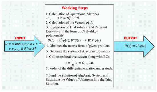
Figure 2.
The flow chart of the algorithm.
5.3. Applications and Discussion
The section is devoted to a comprehensive discussion of obtained results by means of proposed method. The solutions are obtained via both approximate and exact operational matrices-based algorithms and efficiency of the method is verified by means of some numerical examples with various orders of fractional or integer order DEs. The simulations are performed by using Maple 2017. The graphical representation as well as a comparative study with exact solution and existing literature of the problems understudy is being made to show the appropriateness of the algorithms.
Problem 1.
Consider the NMOFDE.
Subject to the initial conditions (ICs) and source term:
The solution of the Problem 1 is obtained forwhile the derivative orders are taken as,[39,40]. The D in the initial conditions is representing derivative w.r.t time. The solutions by means of using CPM viaandare obtained forand 100 digits are taken to the account. Firstly, we obtained operational matrices of derivatives as given below:
where, and are respectively representing exact and approximate operational matrices of derivatives having a fractional order. The polynomial vector of order 4 for is as follows:
The proposed methodology in the previous section is adopted to examine the problem understudy and graphical illustration is with the help of set of graphs while a tabular form (see Table 1, Table 2 and Table 3) of comparison is presented with exact solution and previous literature [39,40]. It is noted that the CPM via brings more accurate and efficient results as compared to CPM via which is clear from the graphical plots. The Figure 3a is plotted for and One can observe that the CPM via is in excellent agreement with the exact solution while the CPM via converges to the exact solution as the value of increases. The Figure 3b is plotted for integer values of derivatives and CPM by means of both kinds of OMs found in good agreement with exact solution which can also be noted form the last two columns of Table 2. The Table 1 and Table 3 are constructed for various values of fractional derivatives to show a comparative analysis between CPM via both kinds of OMs. The Figure 4a is illustrated for the same purpose wherein we can observe that CPM via is more efficient as compared to CPM via It is witnessed from the Figure 4b that method using exact operational matrices still provides an exact solution for higher domain. It is important to highlight that the methods are depending on the developed operational matrices of derivatives. If we use the new operational matrix of derivative i.e., , the accuracy of the method is improved at tangible level for any arbitrary values of fractional derivatives. On the other hand, the method depending on contains errors which could be minimized by taking higher values of

Table 1.
Comparative analysis between algorithms based on both kinds of operational matrices and when and various values of .
Table 2.
Comparative analysis of Problem 1 with exact solution and solutions obtained via Chelyshkov polynomial method (CPM) via and when .
Table 3.
Comparative analysis between algorithms based on both kinds of operational matrices and when and various values of .
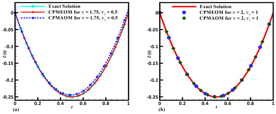
Figure 3.
The graphical representation (Problem 1) exact solution, Chelyshkov polynomial method (CPM) solution via and CPM soliton via . (a). Comparison for fractional order derivatives. (b). Comparison for integer order derivative.
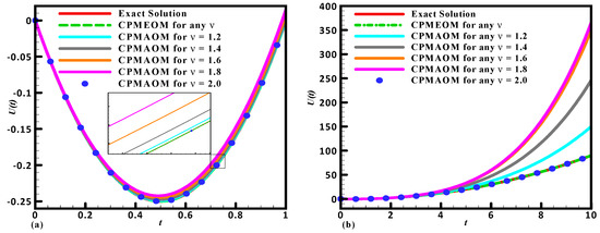
Figure 4.
The graphical representation of (Problem 1) exact solution, CPM solution via and CPM soliton via . The values of are chosen as (a) For and (b) For and .
Problem 2.
Consider the nonlinear multi-order fractional ordinary differential equation (NMOFDE) [39,40].
Subject to the initial conditions (ICs) and source term:
The analysis of Problem 2 under study is reported forwhile the values of coefficientsandare considered as 1. The simulations are being made forand digits = 100. The operational matrices via both approaches has been computed for above mentioned values of fractional order derivatives and stated under:
In the above expressions, and are respectively representing approximate and exact operational matrices of derivatives having a fractional order while the Chelyshkov polynomial vector of order 3 for is stated under:
Again, exact solution is obtained using the algorithm based on while the algorithm based on still contains errors. The Figure 5a is presented to show the graphical behavior of the all three solutions. The tabular form of comparison is also included in the study. One can observe (see Table 4) for small values of N the error is decreased at a tangible level via the proposed method.
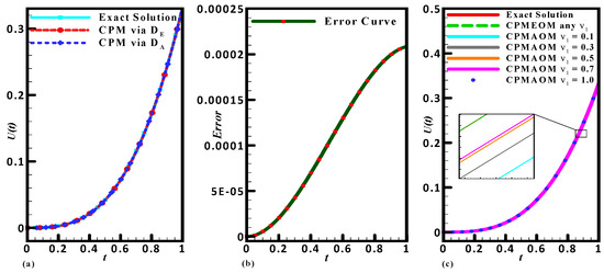
Figure 5.
The graphical representation of Problem 1 exact solution, CPM solution via and CPM soliton via (a) When are integer and (b) Error curve for CPMAOM. (c) Comparative study for different orders of derivatives.
Table 4.
Comparative analysis between algorithms based on both kinds of operational matrices and when and various values of .
The last column of the Table 5 witnesses that no error is found via CPMEOM. The readers can notice that for integer values of derivative involving both algorithms provide the same level of accuracy. The Figure 5b is an error curve for CPM via which is gradually decreasing. The Table 4 and Table 6 are presented for various values of fractional derivatives and ensure the credibility of the newly developed OM while, the Figure 5c is plotted to show the comparison with exact solution for arbitrary values of fractional derivatives. In account of set of graphs and tabular comparison, the suggested algorithm is found as an efficient tool to examine multi-order nonlinear problems of physical and complex nature.
Table 5.
Comparative analysis of Problem 2 with exact solution, existing literature and solutions obtained via Chelyshkov polynomial method (CPM) via and when
Table 6.
Comparative analysis between algorithms based on both kinds of operational matrices and when and various values of .
Bagley–Torvik (BT) Problem Fractional Order
The Bagley–Torvik (BT) equations are considered as an enormously essential part to examine the performance of various materials through the applications of fractional calculus and fractional differential equations [41,42]. It has increased its importance in various disciplines of industry, engineering and applied sciences. In the past, the said problem has been modeled for fractional orders or while the problem arises in frequency dependent damping materials.
Problem 3.
The mathematical form of Bagley–Torvik equation is stated in [41,42].
Subject to the initial conditions (ICs), boundary conditions (BCs) and source term:
In the above expressions (51)–(53), the nonlinear operator and unknown function are represented as and The constant is span input in the interval The constant coefficients are indicted as while are contents. The BT-equation also appear in the neural networking specifically in feed-forward artificial neural network (FFA-NN) and its graphical sketch is presented in the Figure 1. In addition, it is important to highlight that the said problem arises in fractional calculus as a fractional differential equation in neural networks (FDE-NNs). Readers are referred to see [41] for more details about said physical fractional problem of complex nature. It is noted that mathematical formulation of aforementioned problem is the linear combination of the discussed networks while the solution of unknown function could be appropriate unknown weights. In account of this presented model the numerical experiments have been performed when digits = 100, and the orders of derivatives are taken as:
The operational matrices via both approaches have been computed for above mentioned values of fractional order derivatives and stated under:
In the above expressions, and are respectively representing approximate and exact operational matrices of derivatives having a fractional order while the Chelyshkov polynomial vector of order 3 for is stated under:
The proposed scheme is adopted to examine the solution of physical problem understudy and noted that an exact solution is obtained using CPMEOM method for a very small value of N while the CPMAOM contains some error, which is asserted by means of graph (see Figure 6a) and tabular form of the comparative study is given in the Table 7. The graphical illustration of error analysis is presented in Figure 6b. The accuracy level of proposed technique is examined by calculating the L2, L∞ and root mean square (RMS) errors while their descriptions are given below.
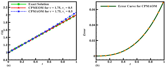
Figure 6.
The graphical representation of Bagley–Torvik (BT)-equation. (a) Exact solution, CPM solution via and CPM solution via . (b) Error curve for CPMAOM.
Table 7.
Comparative analysis between algorithms based on both kinds of operational matrices and when and various values of .
The Table 8, Table 9 and Table 10 are constructed to present the analysis about L2, L∞ and root mean square (RMS) errors while it is noticed that when increasing the number of nodes (10, 102, 500 and 103) we are obtaining better rate of accuracy for CPM via but the CPM via is free of error due to the accuracy of the operational matrix. Hence, we found very efficient and accurate results by means of Chelyshkov polynomial method based on exact operational matrices of derivative (CPMEOM). The set of graphs and tabular forms of comparison are endorsing the credibility and efficiency of the novel matrix−based proposed method and could be extended for the problems arising in engineering and nonlinear sciences.
Table 8.
L2 error analysis for various values of time and comparison between both kinds of methods.
Table 9.
L∞ error analysis for various values of time and comparison between both kinds of methods.
Table 10.
Root mean square (RMS) error analysis for various values of time and comparison between both kinds of methods.
6. Conclusions
The current work is dedicated to the construction of a new computational algorithm based on operational matrices of derivatives. The OMDs are obtained through Chelyshkov polynomials and piecewise functions. A novel mathematical method is proposed depending upon developed matrices and successfully applied for some class of FDEs. The error bound and convergence analysis is reported to validate the consistency of the mathematical structure of CPM.
Hence, some concluding remarks are stated below:
- The matrices are derived by means of two different approaches. The operational matrices obtained via Theorem 1 are approximate for non-integer orders of derivative but exact for any integer order derivative while the Theorem 3 provides the exact operational matrices for both inter and non-integer derivatives. The second tactic was extra effectual and consistent.
- The solutions of the non-integer order problem have been attained via suggested method and very productive results have been attained. In account of obtained results, it is noticed that the CPM has an enhanced accuracy and efficiency rate compared with data in the literature.
- It is also perceived that computational procedure is a well-organized mathematical tool to scrutinize the fractional order problems. Hence, we developed the mentioned method for a class of nonlinear fractional problems and applications in neural networking systems have been reported. The work is extendable to other applied and natural sciences problems.
Author Contributions
Conceptualization, M.H., M.U. and W.W.; methodology, M.H.; M.U., software, M.H., M.U.; validation, M.H., M.U.; formal analysis, M.H., M.U.; investigation, M.H.; M.U., writing—original draft preparation, M.H., M.U.; writing—review and editing, O.M.F.; visualization, I.K.; supervision, M.U., W.W.; project administration, I.K., O.M.F.; funding acquisition, O.M.F. All authors have read and agreed to the published version of the manuscript.
Funding
This research is funded by YUTP (Cost Center 015LC0-173).
Acknowledgments
The authors would like to thank YUTP (Cost Center 015LC0-173) for the financial support in this research. The first author (M. Hamid) is grateful to the Fudan University for providing research opportunities in China through International Exchange Post-Doctoral Fellowship. The author M. Usman acknowledge the support of Peking University through the Boya Post-doctoral Fellowship.
Conflicts of Interest
All the authors declare that there is no actual or potential conflict of interest including any financial, personal or other relationships with other people or organizations.
References
- Oldham, K.; Spanier, J. The Fractional Calculus Theory and Applications of Differentiation and Integration to Arbitrary Order; Elsevier: Amsterdam, The Netherlands, 1974; Volume 111. [Google Scholar]
- Rudolf, H. Applications of Fractional Calculus in Physics; World Scientific: Singapore, 2000. [Google Scholar]
- Raza, J.; Mebarek-Oudina, F.; Mahanthesh, B. Magnetohydrodynamic flow of nano Williamson fluid generated by stretching plate with multiple slips. Multidiscip. Model. Mater. Struct. 2019, 15, 871–894. [Google Scholar] [CrossRef]
- Raza, J.; Mebarek-Oudina, F.; Ram, P.; Sharma, S. MHD flow of non-Newtonian molybdenum disulfide nanofluid in a converging/diverging channel with Rosseland radiation. Defect Diffus. Forum 2020, 401, 92–106. [Google Scholar] [CrossRef]
- Mahanthesh, B.; Lorenzini, G.; Oudina, F.M.; Animasaun, I.L. Significance of exponential space—and thermal—dependent heat source effects on nanofluid flow due to radially elongated disk with Coriolis and Lorentz forces. J. Therm. Anal. Calorim. 2019, 1–8. [Google Scholar] [CrossRef]
- Kreyszig, E. Introductory functional analysis with applications; Wiley: New York, NY, USA, 1978; Volume 1. [Google Scholar]
- Diethelm, K. The Analysis of Fractional Differential Equations: An Application-Oriented Exposition Using Differential Operators of Caputo Type; Springer Science & Business Media: Berlin, Germany, 2010. [Google Scholar]
- Kilbas, A.A.A.; Srivastava, H.M.; Trujillo, J.J. Theory and Applications of Fractional Differential Equations; Elsevier Science Limited: Amsterdam, The Netherlands, 2006; Volume 204. [Google Scholar]
- Sabatier, J.; Agrawal, O.P.; Machado, J.T. Advances in Fractional Calculus; Springer: Berlin, Germany, 2007; Volume 4. [Google Scholar]
- Mainardi, F. Fractional Calculus and Waves in Linear Viscoelasticity: An Introduction to Mathematical Models; World Scientific: Singapore, 2010. [Google Scholar]
- Sun, H.; Zhang, Y.; Baleanu, D.; Chen, W.; Chen, Y. A new collection of real world applications of fractional calculus in science and engineering. Commun. Nonlinear Sci. Numer. Simul. 2018, 64, 213–231. [Google Scholar] [CrossRef]
- Hamid, M.; Usman, M.; Zubair, T.; Mohyud-Din, S.T. Comparison of Lagrange multipliers for telegraph equations. Ain Shams Eng. J. 2018, 9, 2323–2328. [Google Scholar] [CrossRef]
- Podlubny, I.; Skovranek, T.; Datsko, B. Recent advances in numerical methods for partial fractional differential equations. In Proceedings of the 15th International Carpathian Control Conference (ICCC), Velke Karlovice, Czech Republic, 28–30 May 2014; pp. 454–457. [Google Scholar]
- Pedas, A.; Tamme, E. Numerical solution of nonlinear fractional differential equations by spline collocation methods. J. Comput. Appl. Math. 2014, 255, 216–230. [Google Scholar] [CrossRef]
- Bhrawy, A.; Alhamed, Y.; Baleanu, D.; Al-Zahrani, A. New spectral techniques for systems of fractional differential equations using fractional-order generalized Laguerre orthogonal functions. Fract. Calc. Appl. Anal. 2014, 17, 1137–1157. [Google Scholar] [CrossRef]
- Hamid, M.; Usman, M.; Zubair, T.; Haq, R.U.; Shafee, A. An efficient analysis for N-soliton, Lump and lump–kink solutions of time-fractional (2 + 1)-Kadomtsev—Petviashvili equation. Phys. A Stat. Mech. Appl. 2019, 528, 121320. [Google Scholar] [CrossRef]
- Usman, M.; Hamid, M.; Zubair, T.; Haq, R.U.; Wang, W. Operational-matrix-based algorithm for differential equations of fractional order with Dirichlet boundary conditions. Eur. Phys. J. Plus 2019, 134, 279. [Google Scholar] [CrossRef]
- Zeid, S.S. Approximation methods for solving fractional equations. Chaos Solitons Fractals 2019, 125, 171–193. [Google Scholar] [CrossRef]
- Farhan, M.; Omar, Z.; Mebarek-Oudina, F.; Raza, J.; Shah, Z.; Choudhari, R.; Makinde, O. Implementation of one step one hybrid block method on nonlinear equation of the circular sector oscillator. Comput. Math. Model. 2020, 31. [Google Scholar] [CrossRef]
- Alkasassbeh, M.; Omar, Z.; Mebarek-Oudina, F.; Raza, J.; Chamkha, A. Heat transfer study of convective fin with temperature-dependent internal heat generation by hybrid block method. Heat Transf. Asian Res. 2019, 48, 1225–1244. [Google Scholar] [CrossRef]
- Hamrelaine, S.; Mebarek-Oudina, F.; Sari, M.R. Analysis of MHD Jeffery Hamel flow with suction/injection by homotopy analysis method. J. Adv. Res. Fluid Mech. Therm. Sci. 2019, 58, 173–186. [Google Scholar]
- Saadatmandi, A.; Dehghan, M.J.C.; Applications, M.W. A new operational matrix for solving fractional-order differential equations. Comput. Math. Appl. 2010, 59, 1326–1336. [Google Scholar] [CrossRef]
- Doha, E.; Bhrawy, A.; Ezz-Eldien, S. Efficient Chebyshev spectral methods for solving multi-term fractional orders differential equations. Appl. Math. Model. 2011, 35, 5662–5672. [Google Scholar] [CrossRef]
- Doha, E.; Bhrawy, A.; Ezz-Eldien, S. A new Jacobi operational matrix: An application for solving fractional differential equations. Appl. Math. Model. 2012, 36, 4931–4943. [Google Scholar] [CrossRef]
- Mohyud-Din, S.; Iqbal, M.; Hassan, S. Modified Legendre wavelets technique for fractional oscillation equations. Entropy 2015, 17, 6925–6936. [Google Scholar] [CrossRef]
- Bazm, S.; Hosseini, A. Numerical solution of nonlinear integral equations using alternative Legendre polynomials. J. Appl. Math. Comput. 2018, 56, 25–51. [Google Scholar] [CrossRef]
- Usman, M.; Hamid, M.; Haq, R.U.; Wang, W. An efficient algorithm based on Gegenbauer wavelets for the solutions of variable-order fractional differential equations. Eur. Phys. J. Plus 2018, 133, 327. [Google Scholar] [CrossRef]
- Usman, M.; Hamid, M.; Zubair, T.; Haq, R.U.; Wang, W.; Liu, M. Novel operational matrices-based method for solving fractional-order delay differential equations via shifted Gegenbauer polynomials. Appl. Math. Comput. 2020, 372, 124985. [Google Scholar] [CrossRef]
- Usman, M.; Hamid, M.; Khalid, M.S.U.; Haq, R.U.; Liu, M. A robust scheme based on novel-operational matrices for some classes of time-fractional nonlinear problems arising in mechanics and mathematical physics. Numer. Methods Partial. Differ. Equ. 2020, 1–35. [Google Scholar] [CrossRef]
- Usman, M.; Zubair, T.; Hamid, M.; Haq, R. Novel modification in wavelets method to analyze unsteady flow of nanofluid between two infinitely parallel plates. Chin. J. Phys. 2020, 66, 222–236. [Google Scholar] [CrossRef]
- Hamid, M.; Usman, M.; Haq, R.U. Wavelet investigation of Soret and Dufour effects on stagnation point fluid flow in two dimensions with variable thermal conductivity and diffusivity. Phys. Scr. 2019, 94, 115219. [Google Scholar] [CrossRef]
- Mohammadi, F.; Moradi, L.; Baleanu, D.; Jajarmi, A. A hybrid functions numerical scheme for fractional optimal control problems: Application to nonanalytic dynamic systems. J. Vib. Control 2018, 24, 5030–5043. [Google Scholar] [CrossRef]
- Moradi, L.; Mohammadi, F.; Baleanu, D. A direct numerical solution of time-delay fractional optimal control problems by using Chelyshkov wavelets. J. Vib. Control 2019, 25, 310–324. [Google Scholar] [CrossRef]
- Chelyshkov, V.S. Alternative orthogonal polynomials and quadratures. Electron. Trans. Numer. Anal. 2006, 25, 17–26. [Google Scholar]
- Gokmen, E.; Yuksel, G.; Sezer, M. A numerical approach for solving Volterra type functional integral equations with variable bounds and mixed delays. J. Comput. Appl. Math. 2017, 311, 354–363. [Google Scholar] [CrossRef]
- Hamid, M.; Usman, M.; Zubair, T.; Haq, R.; Wang, W. Innovative operational matrices based computational scheme for fractional diffusion problems with the Riesz derivative. Eur. Phys. J. Plus 2019, 134, 484. [Google Scholar] [CrossRef]
- Talaei, Y.; Asgari, M. An operational matrix based on Chelyshkov polynomials for solving multi-order fractional differential equations. Neural Comput. Appl. 2018, 30, 1369–1376. [Google Scholar] [CrossRef]
- Hamid, M.; Usman, M.; Haq, R.; Wang, W. A Chelyshkov polynomial based algorithm to analyze the transport dynamics and anomalous diffusion in fractional model. Phys. A Stat. Mech. Appl. 2020, 551, 124227. [Google Scholar] [CrossRef]
- Yuanlu, L. Solving a nonlinear fractional differential equation using Chebyshev wavelets. Commun. Nonlinear Sci. Numer. Simul. 2010, 15, 2284–2292. [Google Scholar]
- Heydari, M.; Hooshmandasl, M.; Cattani, C. A new operational matrix of fractional order integration for the Chebyshev wavelets and its application for nonlinear fractional Van der Pol oscillator equation. Proc. Math. Sci. 2018, 128, 26. [Google Scholar] [CrossRef]
- Diethelm, K.; Ford, J. Numerical solution of the Bagley-Torvik equation. BIT Numer. Math. 2002, 42, 490–507. [Google Scholar]
- Zubair, T.; Sajjad, M.; Madni, R.; Shabir, A. Hermite Solution of Bagley-Torvik Equation of Fractional Order. Int. J. Mod. Nonlinear Theory Appl. 2017, 6, 104–118. [Google Scholar] [CrossRef][Green Version]


© 2020 by the authors. Licensee MDPI, Basel, Switzerland. This article is an open access article distributed under the terms and conditions of the Creative Commons Attribution (CC BY) license (http://creativecommons.org/licenses/by/4.0/).