Article

On the Loss of Learning Capability Inside an Arrangement of Neural Networks: The Bottleneck Effect in Black-Holes

1
School of Science and Technology and IIBG, The Open University of Hong Kong, 30 Good Shepherd St., Kowloon, Hong Kong, China
2
Department of Computer Science, University of Illinois at Chicago, 851 South Morgan Street, Chicago, IL 60607-7053, USA
*
Author to whom correspondence should be addressed.
Symmetry 2020, 12(9), 1484; https://doi.org/10.3390/sym12091484
Submission received: 5 July 2020 / Revised: 4 September 2020 / Accepted: 6 September 2020 / Published: 10 September 2020

Abstract

:
We analyze the loss of information and the loss of learning capability inside an arrangement of neural networks. Our method is based on the formulation of the Bogoliubov transformations in order to connect the information between different points of the arrangement. Similar methods translated to the physics of black-holes, reproduce the Hawking radiation effect. From this perspective we can conclude that the black-holes are objects reproducing naturally the bottleneck effect, which is fundamental in neural networks in order to perceive the useful information, eliminating in this way the noise.

1. Introduction

Artificial neural networks were proposed for the first time in 1943 as an attempt to simulate the way the human brain operates [1]. By then, the logic, taken as the way how some input information is interpreted, was the key ingredient for the formulation of this concept. Subsequently, the notions of Hebbian learning were developed [2]. The Hebbian network was after analyzed in [3]. The perceptron was proposed in 1958 by Rosenblatt by assuming that there exists a bridge between psychology and biophysics. The perceptron is based on three fundamental questions: 1. How is information about the physical world sensed or detected, by the biological system? 2. In which form is information stored or remembered? 3. How does information contained in storage or memory, influence recognition and behavior?
By complementing the perceptrons with connections (synapses in biological terms), and by taking the output of a neuron as the input of another one, we create a primitive arrangement of neural networks. Although this is a good starting point, it is difficult for an arrangement of neural networks based on perceptrons to learn in the sense of Machine Learning. The reason is that when we use perceptrons, a small change on the input can create huge changes on the output, destroying in many cases the possibility of learning [4]. When a system of neural networks learns, normally it makes improvements based on variations of the weights (importance of the information transmitted through the synapses) and the bias (related to the threshold). Examples of this can be found in the implementation of the method of gradient descend to minimize the cost-function [5,6,7]. In such a case, the perceptrons would operate terribly because any attempt in learning some specific output information belonging to a single output neuron, might destroy easily what the system has learned in order to display some specific outputs corresponding to the other neurons. This situation can be solved by introducing an activation function f ( x ) different to the standard step function in this scenario. The most common non-trivial activation function used is the sigmoid function and here we will take it as the ideal output of a single neuron. The biggest advantage of the sigmoid function is its high sensitivity in responding to small changes in the inputs. This means that it can map small input changes into small output changes. Those small changes might be entered through variations of the weights and bias. In this way, the neural network will be able to learn by updating these values until it gets the desired result. Normally the process of learning is based on the minimization of the cost function. Once the system learns something, ideally it does not forget it and the information is in principle preserved. Excessive information in the system can generate noise which makes it difficult to read the appropriate output. Then some information must be cleared such that the system is able to generate appropriately the desired performance. This, in Machine Learning, is known as the bottleneck effect and it is very important for a system to give results in which humans are able to interpret [8,9].
On the other hand, the black-holes are objects hiding the information [10]. The black-holes not only absorb matter (hiding information) but they also emit it in the form of (Hawking) radiation [11]. Previously, it was demonstrated a generic connection between black-holes and neural networks [12,13,14,15,16]. An initial approach to the evaporation process from this perspective was done in [17,18]. Subsequently, one of the authors analyzed the black-hole evaporation from the perspective of neural networks [19]. Given the fact that black-holes are the objects able to store the information in the most efficient way [12,13,14,15,16], summed to the fact that they also hide the information [10], then it is expected to find a similar effect to the bottleneck effect inside the black-hole physics.
In this paper, we demonstrate that the black-hole “information paradox” is a necessary condition in order to reproduce the bottleneck effect in black-holes. From this perspective, the black-holes clean the information in order to keep it in the most organized form (no hair theorem) [20]. This is precisely what gives stability to these exotic objects. Viewed as a neural network arrangement, the Hawking radiation reproduces naturally a sigmoid-like (with some modification when the particles evaporating are bosons) activation function. If the Hawking radiation were able to reproduce instead a perceptron-like function (behavior), then the black-hole would be a very unstable object, unable to radiate until it accumulates some activation energy, after which a catastrophic explosion emitting the whole information from inside would occur. Fortunately, the stability of the black-holes is guaranteed by the bottleneck effect. The methods exposed here can be used for analyzing the bottleneck effect in neural networks in a general framework by using the standard Bogoliubov transformations [21,22].
The paper is organized as follows: In Section 2, we introduce the basic concept of perceptrons, understanding that the activation function is a step function in such a case. In Section 3, we explain the neural network arrangement using the sigmoid as an activation function. In Section 4, we explain the generic map between the degrees of freedom of a quantum field and the degrees of freedom of a neural network arrangement. In Section 5, we analyze the evolution of the information inside a neural network arrangement. We then explain how the information can be reduced such that the appropriate activation function appears. This result comes out to be equivalent to the result derived by Hawking in [11], for the analysis of the black-hole evaporation, but considering massless fermions, such as neutrinos for example. Connecting the information from one point of the arrangement to the next, can be achieved by using Bogoliubov transformations [21,22]. In Section 6, we explain how the black-holes reproduce the bottleneck effect naturally in order to guarantee stability. Finally, in Section 7, we conclude.

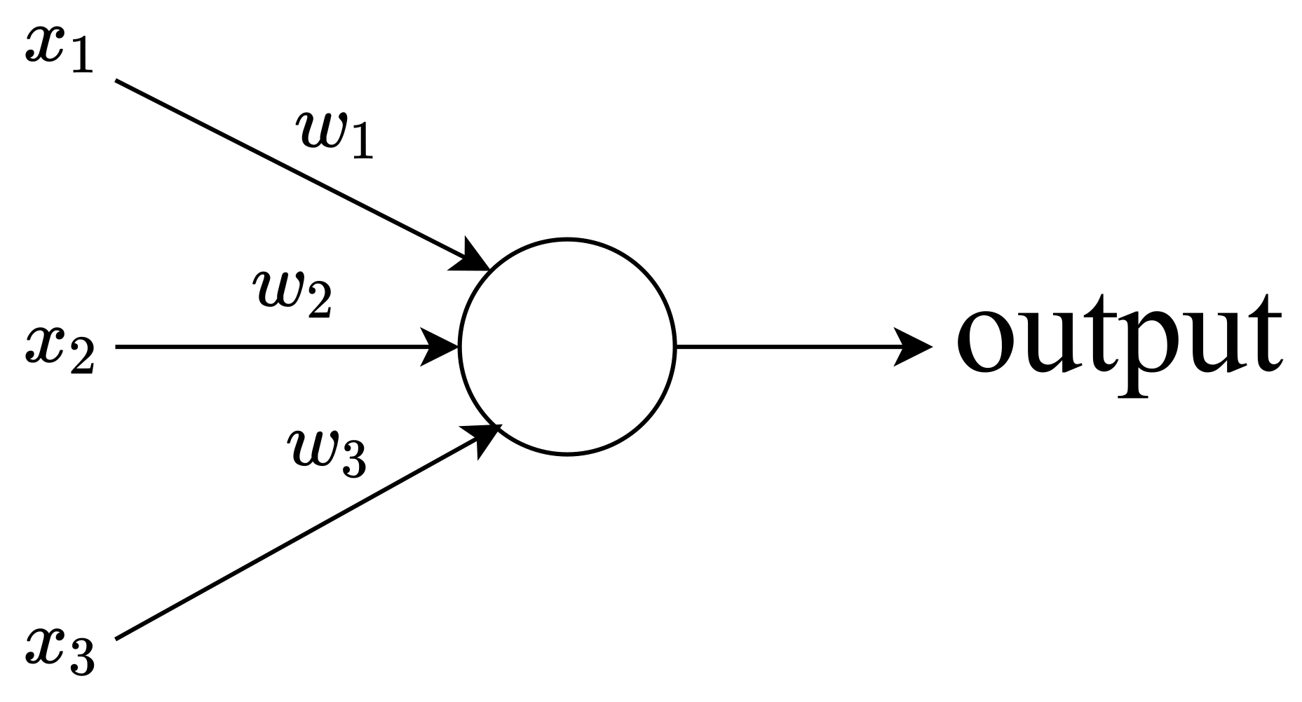
2. Perceptrons: Basic Concepts

We start the paper with the basic definition of neural networks, by considering each neuron to be equivalent to a perceptron in the form originally proposed in [1]. A perceptron takes different inputs defined by a set of variables x 1 , x 2 , x 3 , x n and it reproduces a single binary output [4]. The neuron in such a case reproduces some specific output m j defined by either, m j = 0 or m j = 1 ( j = 1 , 2 , 3 , is the number of output neurons), depending on whether or not the weighted sum of inputs is larger or not than some specified threshold. The threshold can also appear in the form of bias. Specifically, the condition imposed over the perceptrons is
f ( x j ) = m j = 0 , i f j ω j x j + b 0 = 1 , i f j ω j x j + b > 0
where b corresponds to the bias of the perceptron and it is equivalent to the threshold of the neuron, ω j are the weights and f ( x j ) is the activation function for each neuron in the arrangement. Figure 1 illustrates the standard behavior of a perceptron neuron.
We can perceive the perceptron as a neuron able to take a decision based on input weighted evidence. From the perspective of biological neurons, the weights w j defined in Equation (1) represent the importance which the synapse gives to the different input patterns. One example with two weights can be the decision of drinking/not drinking coffee in the morning. We can assume that the output f ( x j ) = 0 means drinking coffee and the output f ( x j ) = 1 means drinking milk in the morning. We can then take the first binary input as x 1 = 1 if the person who will take the decision has some heart problems (hypertension) and x 1 = 0 if there are no such health problems. Similarly, we might take the second input as x 2 = 1 if the person who will take the decision suffers insomnia and x 2 = 0 if this is not the case. Based on that, our system will decide if it is appropriate to drink milk or coffee during a breakfast in the morning. Our system could give weights to the pair of binary inputs, let us take the same weights for both inputs as w 1 = 2 and w 2 = 2 . This means that both inputs are equally important for the system. If we take the bias to be equivalent to b = 3 , then in agreement with Equation (1), the system will decide that the person should drink milk in the morning if he/she suffers both, insomnia and hypertension. On the other hand, the system will only decide that coffee is appropriate if: (1). The person suffers hypertension but not insomnia. (2). The person suffers insomnia but not hypertension. (3). The person is completely healthy. In this simple situation, a system with an operation based on perceptrons will be enough. More complex arrangements can be done if we create a more complex network like the one in Figure 2. To show the difficulties that the perceptron neurons have in learning appropriately some specific tasks, we will study now the sigmoid neurons and we will focus on these important aspects of artificial neural networks.

3. Sigmoid Neurons

The sigmoid neurons are different from the perceptrons because the response function of the neurons is not a step function, but rather a sigmoid function defined as
σ ( z ) = 1 1 + e z ,
where z = j ω j x j + b , which is the same entrance used for the perceptrons in Equation (1). Note that the response function can take any real value between 0 and 1 which marks a significant difference from the perceptron case. This corresponds to a huge advantage during the process of learning when the system is compared with the situation where we analyze perceptrons. Note that there are two limits for the sigmoid function where the behavior corresponds to perceptrons. They are z ± , which correspond to σ ( z ) 1 or σ ( z ) 0 . The biggest advantage of the sigmoid function for learning is that small changes in the inputs correspond to small changes in the outputs. This can be quantified mathematically as
Δ m i j m i ω j Δ ω j + m i b Δ b
where m i would correspond to any output which the system provides and we wish to update. Equation (3) only represents the ordinary chain rule taken from calculus. The superiority in learning for neural networks using as a response the sigmoid function, can be seen in the example of a network used for classifying handwritten digits using a three-layer neural network. The input layer of the network contains neurons encoding the values of the input pixels and the output contains 10 neurons, each one representing a different digit from 0 to 9. If the first neuron is excited, then the system will identify 0 for m 0 , if the second output neuron is the one excited, then the system will naturally identify 1 for m 1 and so on. Let us assume that the system has a problem identifying the number 9, i.e., the output neuron, corresponding to the digit 9 ( m 9 ), does not get excited even if the input image is a 9. In other words, for an input 9, the system of computer vision detects m 9 9 . Given this problem, the system would have to be adjusted by changing gradually the weights ω j and bias b, such that the last neuron can shoot for the appropriate case, namely, for the detection of the number 9. This is what we call the process of learning. The small changes in weights and bias will be detected as small changes in the outputs m i in agreement with Equation (3). This gives us then the advantage of testing simultaneously all the other output numbers (from m 0 to m 9 ). Or equivalently, in this way we avoid to damage any adjustment for the other output neurons ( m i ) corresponding to the identification of the other numbers. This clever way of learning is impossible if we use perceptrons because for perceptrons we would have possible drastic changes in the outputs for a finite change in the inputs. Following the same example, consider that we are adjusting the output m 9 in order to detect the number 9 correctly. The only way to do this is by changing simultaneously the weights ω j . However, changing the weights will also generate possible changes for the other outputs m i 9 . For the case of the sigmoid-response function defined in Equation (2), we can always check that the other outputs are still correct after adjustments. For the case of perceptrons, we cannot see what kind of damage we are doing to the other outputs when we are updating the weights. Then, a well-behaved neuron giving an output m 0 = 0 can suddenly gives the result m 0 = 8 or anything else, even if we can correct the output m 9 = 9 . It is for this reason that the possible transitions from the sigmoid response to the perceptron response, as a consequence of the excessive amount of information, deserve careful attention.

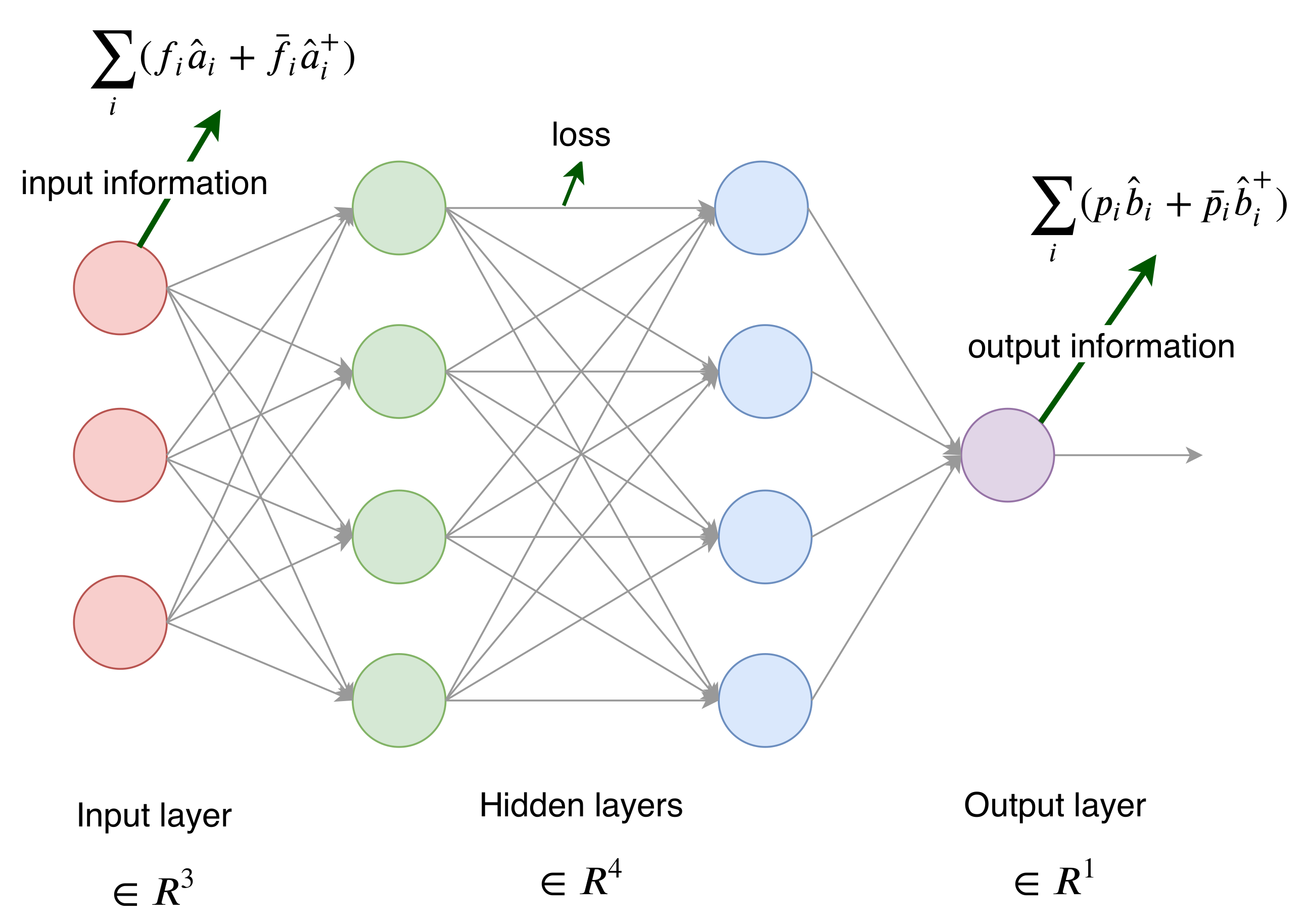
4. The Connection between Neural Networks and Quantum Fields

The connection between neural networks and quantum fields was done in [12,13,14,15,16] and here we review it. The idea is that we can map the degrees of freedom of a quantum field, onto the degrees of freedom of a neural network arrangement. Consider a Bosonic field obeying the usual commutation relations
[ a ^ i , a ^ j + ] = δ i j , [ a ^ i , a ^ j ] = [ a ^ i + , a ^ j + ] = 0 .
The level of excitation is defined by the occupation number n ^ k = a ^ k + a ^ k , with the eigenvalues defined by n ^ k | n k > = ( 0 , 1 , , d 1 ) | n k > and k = 0 , 1 , , K defining the number of degrees of freedom (oscillators). The information is then stored in d K + 1 possible states of the form | n 0 , n 1 , , n K > . The effort for storing information is measured by the difference between the energy levels | n k > and | n k ± 1 > . We can then consider a neural network arrangement where each neuron corresponds to one oscillator with the occupation number n k . The higher the occupation number is, the higher will be the gap associated to the neuron. Under the present analogy, we would have K + 1 neurons and the state representing the storage information pattern is just the same state | n 0 , n 1 , , n K > .

4.1. Assisted Gaplessness

The free Bosonic field defined previously, suggests that the gap between the states | n k > and | n k + 1 > is given by
E n 0 , n 1 , , n K = k E k n k ,
which just corresponds to the difference between eigenvalues when we operate the Hamiltonain over the different states. By using the analogy with neural networks, we can take each neuron to correspond to each degree of freedom for the quantum field. Then each occupation number n k is related to the gap corresponding to the neuron, which measures how much energy we should invest in order to store some patterns of information. Then in principle, since we have K + 1 neurons, we can then store d K + 1 patterns. The higher the gap (5) is, the higher is the difficulty in storing patterns of information. However, when the neurons interact among each other, the effective gap perceived by some neurons can be reduced dramatically depending on the kind of coupling between neurons. This allows then the possibility of getting zero gap and the zero cost for storing patterns. The phenomena allowing the gaps to vanish after interaction between neurons is called “assisted gaplessness”. It is formulated at the most basic level through the interaction between several networks with a single neuron dubbed “master neuron”. The Hamiltonian for a system considering the interaction between a master neuron and several neurons is defined as
H ^ = k = 1 K E k ( 1 α n ^ 0 ) n k ^ + E 0 n 0 ^ .
with higher order terms (not included here) which guarantee the stability of the theory. Note that the last term in Equation (6) corresponds to the gap of the master neuron E 0 n 0 , which is obtained after operating the portion of the Hamiltonian E 0 n ^ 0 over the states | n 0 , n 1 , , n K > . This term appears even for the free-field case defined in Equation (5). The first term in the expansion corresponds to the gaps of all the other neurons, appearing as k E k n k . This terms also appears in the free theory without interactions. The interesting term is the one corresponding to the interaction between neurons and in Equation (6) defined as E k α n ^ 0 n ^ k . Then the sign of α defines whether the interaction reduces the effective gap of all the neurons (except the gap of the master neuron) or not. The effective gap is defined as
E k ( 1 α n ^ 0 ) n k ^ = E k f ^ 0 , k ,
where f ^ 0 , k is just a tensor with two indexes. Note that the effective gap of the neurons vanishes when the tensor f ^ 0 , k = 0 is trivial and this imposes the condition
n 0 = 1 α ,
for the terms obtained from the eigenvalues of the Hamiltonian. Then we can conclude that assisted gaplessness allows the possibility of getting zero cost for storing information patterns in some neural network arrangements. The key question at this point is if all the information appearing in the first layer of neurons is the whole information we can see at the output. Another interesting point is to explore the stability of the gapless states, which was investigated in [17,18].

4.2. Memory Burden

In [17,18], it was analyzed how the modes in the master neuron can be translated toward the modes of another neuron. Here we can analyze this situation if we add additional modes to the Hamiltonian (6) as follows
H ^ = E 0 n ^ 0 + E 0 m ^ 0 + k = 1 K E k ( 1 α n ^ 0 ) n k ^ + C 0 ( a ^ 0 + b ^ 0 + b ^ 0 + a ^ 0 ) +
where C 0 parameterizes the strength of the interaction between the master neuron modes and the new modes under consideration. One of them can be considered empty initially and the other full of information. In this way, we then define the initial state
| ψ > 0 = | N , 0 , n 1 , , n K >
where the master neuron with the quantum number n 0 = N is fully packaged and the modes corresponding to the operators b ^ 0 are empty. The idea is to explore how the modes can go from the master neuron to the empty neuron. An analytical calculation done in [17,18], evaluated the time-dependence of the expectation value of the gap of the master neuron, obtaining then some time-dependence in n 0 ( t ) . It came out that the obtained function had a dependence in the following term
μ = k = 1 K α E k n k .
Note that this quantity vanishes when the neurons represented by n k , have no information. When this happens, evidently, n 0 ( t ) will oscillates freely with maximal amplitude in a time scale C 0 1 . This case then corresponds to empty space in time-average and we should not expect any event horizon in this situation. In other words, there is no black-hole in this case because there is no event horizon. This is the case because n k scales with the area of the event horizon ( k n k A r e a ) in agreement with [12,13,14,15,16]. The story changes when μ 0 , in such a case, if C 0 2 / μ 2 < < 1 , then the amplitude of oscillation is suppressed by the same ratio. Then, the memory burden makes the states where the master neuron is occupied, stable. Some methods for avoiding the memory burden were explored further in [17,18]. We can conclude from this section that the master mode behaves as the black-hole itself in the sense that it is stable due to the memory storage. Interestingly, the information of the black-hole is measured by the number of gapless modes interacting with the master mode. This number coincides with N. Finally, the new neuron, receiving the information from the master mode and defined through the term E 0 m ^ 0 in the Hamiltonian (9), defines the new state where the black-hole is supposed to go. The burden memory only shows that the larger the black-hole is, the more stable is it, which is consistent with the currently known theories. The Hawking radiation would correspond to the modes escaping the system when they try to move from the master neuron to the empty neuron. Then we can say that not all the master modes will appear mapped in the new state of the system. This is indeed an interesting analogy, which deserves further attention in the near future. Another possibility of looking at this scenario is to imagine that the modes b ^ 0 correspond to the modes escaping from the black-hole via quantum depletion (Hawking radiation) [12,13,14,15,16,23].

5. Cleaning the Information in Neural Networks

After looking into the advantages of the sigmoid function over the perceptrons, we explore how the excessive information can be eliminated from a system. Intuitively, we can say that if the system has excessive information, then its learning capability is reduced. In order to increase this capability, it is necessary to extract the noise or the garbage information. When there is excessive information (noise), the appropriate response (activation) function is the perceptron because it requires an activation energy, which we can set over the noise information level for accomplishing a response. However, as we have seen, the perceptron behaves bad for learning purposes. When we eliminate the noise, we can safely use the sigmoid function as the activation function for neurons without any fear in thinking that the noise will affect the output of the system. Here we use the method proposed in [19] and extend it to real scenarios for explaining how the information can be extracted from a system Mathematically. First, we redefine the response (activation) functions as the vacuum expectation value of the particle-number operator related to the existence of a massless quantum scalar field. We define the quantum scalar field expanded as a Fourier series in the form
ϕ ^ 1 ( z ) = k p k ( z ) a ^ k + p ¯ k ( z ) a ^ k + .
This quantum field expansion is general, subsequently we have to impose the algebra which the annihilation and creation operators will obey. If we select the response functions to behave as a system of fermions, then the local algebra is defined by the anti-commutators [24]
{ a ^ k , a ^ k + } = δ k , k
where a ^ k is the annihilation operator for the local vacuum a ^ k | 0 > = 0 and a ^ k + is the creation operator. For a purely fermionic system, we will take the expectation value for the particle number operator to obey the Pauli exclusion principle as [25]
< 0 | n ^ k a | 0 > = < 0 | a ^ k + a ^ k | 0 > = k = n δ ( k ) .
This corresponds to the perceptron statistic, purely fermionic, which means that a neuron (state) can be either not activated < 0 | n ^ k | 0 > = 0 (vacuum) or activated in agreement with < 1 | n ^ k | 1 > = 1 (excited) depending on the received input. Here we will take the vacuum as the state corresponding to the zero eigenvalue occupation number i.e., n k = 0 . δ [ k ] in Equation (14) is the standard delta-Dirac function which characterizes the step function (perceptron) behavior and | 0 > corresponds to the standard vacuum state. Figure 2 shows a point in the network where the information stored in the system obeys the distribution (12). Note that we are taking the step function behavior as the total output of the system when there is excessive information.
In the same way, at another point of the network, we can expand the same scalar field defined in Equation (12) in terms of a different set of modes as
ϕ ^ 2 ( z ) = k f k ( z ) b ^ k + f ¯ k ( z ) b ^ k + .
The scalar field defined in Equation (15) does not have necessarily the same information of the scalar field defined in Equation (12). In a standard form, we will take the algebra of creation and annihilation operators for this field as fixed and being equivalent to
{ b ^ k , b ^ k + } = δ k , k .
In Figure 2, we assume that the information provided by the neuron is lower than the initial information. In this way, the sigmoid function appears safely as the activation function of the neuron. Then the quantum field (15) has a lower amount of information than the original field expanded in Equation (12). Here, we also define another local vacuum condition b ^ k | 0 ¯ > = 0 . Note that the vacuum | 0 > defined by a ^ k is different to the vacuum | 0 ¯ > defined for the b ^ k -operators. This means that in different points of the network we have a different amount of information, and at each point, we define “empty” or “no-information” in a different way. We can then connect the operators defined in Equation (12) with those defined in Equation (15) via Bogoliubov transformations. Then we have the relations
b ^ k = j α ¯ k j a ^ j β ¯ k j a ^ j + ,
with the corresponding complex conjugate. For our purposes, this is the important relation because it is the one which establishes the connection between the local vacuums defined at each point of the arrangement. Note that if β i j = 0 in the previous equation, then the information is preserved and | 0 > = | 0 ¯ > unambiguously. This is the case because in these special circumstances, both operators a ^ k and b ^ k annihilate the same vacuum. For this case, the step (Heaviside) response function will never change into a sigmoid function or vice versa. On the other hand, if β ¯ k j 0 , then | 0 > | 0 ¯ > and the amount of information in the network changes when it evolves through the system. It is possible to obtain the function governing the amount of information for the modes defined in Equation (15). These are the modes ideally perceived by the observers when the system is performing well. For this purpose, we analyze the vacuum expectation value for the particle number
< 0 | n ^ k b | 0 > = | β k j | 2
where the superindex b is telling us that we are evaluating the particle number operator for the b ^ k -modes. Note that in Equation (18), we are evaluating the expectation value with respect to the vacuum defined by the a ^ k -modes. The result (18) comes from the Bogoliubov transformations (17) and taking a ^ k | 0 > = 0 for setting the vacuum behavior. Note that if we evaluate Equation (18) with respect to the vacuum | 0 ¯ > , then we would obtain the trivial result < 0 ¯ | n ^ k b | 0 ¯ > = 0 . We can evaluate explicitly the result (18). We can do this inspired in the work of Hawking for the black-hole evaporation [11] where the same mathematics can be applied. Following the notation in [11], assume for example that a fraction of the modes entering the system is Γ k = k = δ ( k ) (see Equation (14)), corresponding to the full information provided by the field ϕ ^ 1 . A fraction of information 1 Γ k corresponds to the modes never appearing in the problem, just ignored because they never entered the system at all. Here,
Γ k = n ( | α k n | 2 + | β k n | 2 ) .
It can be demonstrated that the only way for getting a sigmoid (Logistic) function from the previous equation, is having the following relation between the Bogoliubov coefficients
| α k n | = e z / 2 | β k n | .
Introducing this result inside Equation (19), we get
| β k n | 2 = Γ k 1 + e z ,
which is proportional to the sigmoid function (it is more properly a Logistic function) and it corresponds to the information displayed by ϕ ^ 2 at the end after the bottleneck effect becomes effective. Note that the result (21) has a correspondence to the Fermi–Dirac statistics distribution [26] for a group of identical fermions in thermodynamic equilibrium. This is a very interesting result. Note that in this conclusion for the result (21), we have used Equation (18). This completes the demonstration. We can search the difference between the information defined by the modes at different points of the network if we evaluate the following
< 0 | n ^ k b n ^ k a | 0 > = f σ ( z ) f p ( z ) = 1 2 t a n h z / 2 + 1 1 2 π s i n h z / 2 d z ( c o s ( k z ) i s i n ( k z ) ) .
This result quantifies the difference Δ n ^ n = n ^ k a n ^ k b , which is related to the amount of information which we need to extract from the system such that we can use the sigmoid function as an activation function in a safe way.

6. The Bottleneck Effect in Black-Holes

The bottleneck effect just explained in this paper is exactly what guarantees the stability of the black-holes. The black-holes are objects able to store the information in the most efficient way [12,13,14,15,16]. The black-holes retain the information and then they start to transmit it back (at least partially) via Hawking radiation. From the perspective of neural networks, if the black-holes were able to transmit the output information by using as an activation function the perceptron, then there would not be any information paradox in black-holes [10] because there would not be any evaporation process at all. Basically the black-hole would never send away any radiation, except after the system reaches an energy higher than the activation energy, provoking then a sudden explosion. This scenario would create a very unstable system in some cases. On the other hand, the standard behavior of a black-hole suggests that it evaporates via Hawking radiation sending away output information behaving as a sigmoid function (more properly a Logistic function). The standard calculation suggests that at the past-null infinity, before the formation of the black-hole, a scalar field can be expanded in agreement with Equation (12). Subsequently, after the formation of the black-hole, the same scalar field can be expanded as
ϕ ( x ) = p f p b ^ p + f ¯ p b ^ p + + q p c ^ p + q ¯ p c ^ p + = ϕ 2 ( x ) + p q p c ^ p + q ¯ p c ^ p + .
The modes f p are those evaporating and perceived by an observer located at the future null infinity. From the perspective of neural networks, those modes are just the output of the system. The standard calculation done by Hawking in [11], suggests that the evaporating modes obey the following distribution
| β k n | 2 = Γ k 1 ± e 2 π ω κ
where the positive sign in the denominator corresponds to the evaporation of fermion modes. The negative sign corresponds to the evaporation of bosons. Compare this previous result with Equation (21). It is evident from these results that the black-holes clean the information via bottleneck effect, transmitting in this way only the necessary amount of information to the environment. From this perspective, the black-hole information paradox is just equivalent to a bottleneck effect via neural networks and it guarantees total stability of the black-holes.

7. Conclusions

Here, we have presented a novel method for analyzing a mechanism for extracting useless information from a neural network arrangement, such that it can recover its learning capability. The method consists of promoting the activation function as the vacuum expectation value of the particle number operator n ^ k , defined by using the annihilation and creation operators from the expansion of the quantum fields. If the information is unchanged in the system, the Bogoliubov coefficient β k j would vanish. On the other hand, a non-trivial value of β k j implies non-conservation of information, allowing then the possibility of extracting noise (useless information) from the system. Cleaning the information in this way allows us to use the sigmoid function as an activation function, with all the advantages which it implies. A similar effect (bottleneck effect) appears in the evaporation process of a black-hole and it is known as Hawking radiation [11]. Note that the map of information from neuron to neuron is carried-out by using the Bogoliubov transformations. These transformations are Mathematically general and they have been used in the standard calculations corresponding to the Hawking radiation [11,19,27]. The take-home message in this work is that if we want to quantify the loss of information in a system, by storing the information in agreement with a quantum field, this can be done by using the Bogoliubov transformation. Note that the extraction of useless information, explored here, is similar (qualitatively) to the methods used for analyzing information developed in [8,9]. In fact, the extraction of information based in the Bottleneck principle explained in [8,9] consists in the elimination of what we interpret as an initial noise. We could use similar techniques to the one showed in this paper for explaining such effect. These comparisons will be reserved for coming papers. Other aspects which deserve to be further explored are the methods proposed in this paper, but developed from the perspective of the memory burden proposed in [17,18]. In this paper, we have discussed part of this phenomena and we understood its complete equivalence to the bottleneck effect proposed here by the authors. However, further details need to be analyzed in coming papers.

Author Contributions

Both authors contribute equally to the article. All authors have read and agreed to the published version of the manuscript.

Funding

This research received no external funding.

Acknowledgments

The authors would like to thank LatinX in AI, particularly to Laura Montoya, Matias Valdenegro, as well as the organizers of the conference Neurips 2019, developed in Vancouver-Canada for the support obtained during the participation in this event. In particular, LatinX in AI sponsored our trips for the multiple events organized within Neurips 2019. This work was presented as a Poster in the LatinX Workshop within Neurips and in another format inside the Workshop Machine Learning and the Physical Sciences 2019.

Conflicts of Interest

The authors declare no conflict of interest.

References

  1. McCulloch, W.; Pitts, W. A Logical Calculus of Ideas Immanent in Nervous Activity. Bull. Math. Biophys. 1943, 5, 115–133. [Google Scholar] [CrossRef]
  2. Hebb, D. The Organization of Behavior; Wiley: New York, NY, USA, 1949; ISBN 978-1-135-63190-1. [Google Scholar]
  3. Farley, B.G.; Clark, W.A. Simulation of Self-Organizing Systems by Digital Computer. IRE Trans. Inform. Theory 1954, 4, 76–84. [Google Scholar] [CrossRef]
  4. Nielsen, M. Neural Networks and Deep Learning. Available online: http://neuralnetworksanddeeplearning.com/ (accessed on 31 August 2019).
  5. Goudet, O.; Duval, B.; Hao, J.K. Gradient Descent based Weight Learning for Grouping Problems: Application on Graph Coloring and Equitable Graph Coloring. arXiv 2019, arXiv:1909.02261. [Google Scholar]
  6. Harvey, N.J.A.; Liaw, C.; Randhawa, S. Simple and optimal high-probability bounds for strongly-convex stochastic gradient descent. arXiv 2019, arXiv:1909.00843. [Google Scholar]
  7. Xie, Y.; Wu, X.; Ward, R. Linear Convergence of Adaptive Stochastic Gradient Descent. arXiv 2019, arXiv:1908.10525. [Google Scholar]
  8. Tishby, N.; Zaslavsky, N. Deep Learning and the Information Bottleneck Principle. arXiv 2015, arXiv:1503.02406. [Google Scholar]
  9. Shwartz-Ziv, R.; Tishby, N. Opening the Black Box of Deep Neural Networks via Information. arXiv 2017, arXiv:1703.00810. [Google Scholar]
  10. Susskind, L. The Black Hole War: My Battle with Stephen Hawking to Make the World Safe for Quantum Mechanics; Little Brown and Company, Hachette Book Group USA: New York, NY, USA, 2008. [Google Scholar]
  11. Hawking, S.W. Particle creation by black holes. Commun. Math. Phys. 1975, 43, 199–220. [Google Scholar] [CrossRef]
  12. Dvali, G. Critically excited states with enhanced memory and pattern recognition capacities in quantum brain networks: Lesson from black holes. arXiv 2017, arXiv:1711.09079. [Google Scholar]
  13. Dvali, G. Area law microstate entropy from criticality and spherical symmetry. Phys. Rev. D 2018, 97, 105005. [Google Scholar] [CrossRef] [Green Version]
  14. Dvali, G. Black Holes as Brains: Neural Networks with Area Law Entropy. arXiv 2018, arXiv:1801.0391. [Google Scholar] [CrossRef] [Green Version]
  15. DVali, G. Classicalization Clearly: Quantum Transition into States of Maximal Memory Storage Capacity. arXiv 2018, arXiv:1804.06154. [Google Scholar]
  16. Dvali, G.; Michel, M.; Zell, S. Finding Critical States of Enhanced Memory Capacity in Attractive Cold Bosons. EPJ Quantum Technol. 2019, 6, 1. [Google Scholar] [CrossRef]
  17. Dvali, G. A Microscopic Model of Holography: Survival by the Burden of Memory. arXiv 2018, arXiv:1810.02336. [Google Scholar]
  18. Dvali, G.; Eisemann, L.; Michel, M.; Zell, S. Black Hole Metamorphosis and Stabilization by Memory Burden. arXiv 2006, arXiv:2006.00011. [Google Scholar]
  19. Arraut, I. Black-hole evaporation from the perspective of neural networks. EPL 2018, 124, 50002. [Google Scholar] [CrossRef] [Green Version]
  20. Israel, W. Event Horizons in Static Vacuum Space-Times. Phys. Rev. 1967, 164, 1776–1779. [Google Scholar] [CrossRef]
  21. Valatin, J.G. Comments on the theory of superconductivity. Il Nuovo Cimento 1958, 7, 843–857. [Google Scholar] [CrossRef]
  22. Bogoliubov, N.N. On a new method in the theory of superconductivity. Il Nuovo Cimento 1958, 7, 794–805. [Google Scholar] [CrossRef]
  23. Arraut, I. Black-Hole evaporation and Quantum-depletion in Bose-Einstein condensates. arXiv 2006, arXiv:2006.09121. [Google Scholar]
  24. Peskin, M.E.; Schroeder, D.V. An Introduction to Quantum Field Theory; CRC Press/Taylor and Francis Group: Boca Raton, FL, USA, 2018. [Google Scholar]
  25. Pauli, W. Über den Zusammenhang des Abschlusses der Elektronengruppen im Atom mit der Komplexstruktur der Spektren. Z. Phys. 1925, 31, 765–783. [Google Scholar] [CrossRef]
  26. Pathria, R.K.; de Beale, P. Statistical Mechanics; Elsevier: Amsterdam, The Netherlands, 1996. [Google Scholar]
  27. Farley, A.N.S.J.; D’Eath, P.D. Bogoliubov transformations for amplitudes in black-hole evaporation. Phys. Lett. B 2005, 613, 181–188. [Google Scholar] [CrossRef] [Green Version]
Figure 1. Perceptron neuron with three input variables and a single output 0 or 1. The inputs are represented by x 1 , x 2 and x 3 . Here, ω i are the weights corresponding to each input.
Symmetry 12 01484 g001
Figure 2. Standard neural network. The information flows from the input to the output. For perceiving the relevant information, it is necessary to have a loss of information during the transmission through the synapses as the figure illustrates. We take the input information as the one stored in a quantum field. The system starts behaving as a perceptron expanded by the modes obeying the algebra { a ^ k , a ^ k + } = δ k , k and it becomes a sigmoid expanded by the modes obeying { b ^ k , b ^ k + } = δ k , k after extracting the information.
Symmetry 12 01484 g002

