Picture Fuzzy Geometric Aggregation Operators Based on a Trapezoidal Fuzzy Number and Its Application

Abstract

The picture fuzzy set is a generation of an intuitionistic fuzzy set. The aggregation operators are important tools in the process of information aggregation. Some aggregation operators for picture fuzzy sets have been proposed in previous papers, but some of them are defective for picture fuzzy multi-attribute decision making. In this paper, we introduce a transformation method for a picture fuzzy number and trapezoidal fuzzy number. Based on this method, we proposed a picture fuzzy multiplication operation and a picture fuzzy power operation. Moreover, we develop the picture fuzzy weighted geometric ($PFWG$) aggregation operator, the picture fuzzy ordered weighted geometric ($PFOWG$) aggregation operator and the picture fuzzy hybrid geometric ($PFHG$) aggregation operator. The related properties are also studied. Finally, we apply the proposed aggregation operators to multi-attribute decision making and pattern recognition.

1. Introduction

Multi-attribute decision making and pattern recognition problems are widely used in economy, politics, culture and other fields. Because of the ambiguity and complexity of information, it is very difficult for people to evaluate attributes with real numbers. Fuzzy set theory can be used to deal with fuzzy information effectively, which has attracted the attention of many scholars in fuzzy set theory, and it is applied in many fields. In the process of solving multi-attribute decision and pattern recognition problems, information aggregation is a common activity. Among which, weighted aggregation operators, ordered weighted aggregation operators and hybrid aggregation operators are three common aggregation operators.

1.1. Introduction for Picture Fuzzy Sets

Zadeh [1] proposed fuzzy set, which can deal with fuzziness information by membership degree. Fuzzy sets are limited in dealing with fuzziness and uncertainty of information. Atanassov [2,3] proposed intuitionistic fuzzy set, as directly extension of fuzzy set, which presents information by membership degree, non-membership degree, and the sum of two membership degrees less than or equal to one. Intuitionistic fuzzy sets can better describe fuzziness and uncertainty of information. Many scholars have done a lot of research for deal with uncertain of information under the intuitionistic fuzzy environment, such as: distance measures [4,5], similarity measures [6,7,8], aggregation operators [9,10,11], accuracy function and score function [12]. However, intuitionistic fuzzy sets are limited in dealing with inconsistency, uncertainty and fuzziness of information. For example, voting questions. The results of the vote were divided into yes, abstention, against and refusal. For solving these types of problem, Cuong and Kreinovich [13] proposed picture fuzzy set, as directly extension of intuitionistic fuzzy set, which presents information by positive membership degree, neutral membership degree, negative membership degree, and the sum of three membership degrees less than or equal to one. The picture fuzzy sets can dealing with inconsistency, uncertainty and fuzziness of information. Many scholars have also done a lot of research on the theory and application under the picture fuzzy environment. Son [14] proposed generalized picture fuzzy distance measure and applied to clustering problem of picture fuzzy sets. Dinh [15] proposed dissimilarity measure and distance measure of picture fuzzy sets. Guleria and Bajaj [16] proposed picture fuzzy probabilistic distance measure and applied to classification problems. Wei [17] proposed some similarity measures of picture fuzzy sets. Wei [18,19] proposed cross-entropy and 2-tuple linguistic aggregation operators for picture fuzzy and applied them to multi-attribute decision making. Joshi [20] propose information measure of picture fuzzy sets and applied them to decision making.

1.2. The Development State for Picture Fuzzy Aggregation Operators

In the process of information aggregation, the aggregation operators are important tools. Based on the family of t-norm and t-conorm, many aggregation operators of picture fuzzy sets have been proposed. Jana [21] proposed picture fuzzy Dombi aggregation operators. Wei [22] proposed picture fuzzy Hamacher aggregation operators and applied them to multi-attribute decision making. Jana [23] applied picture fuzzy Hamacher aggregation operators to assess the best enterprise. Garg [24] proposed some picture fuzzy aggregation operators based on a decreasing function generates the t-norm and t-conorm. Ashraf [25] proposed picture fuzzy aggregation operators by using algebraic and Einstein t-norm and t-conorm, applied them to multi-attribute decision making. Wang et al. [26] proposed some picture fuzzy geometric aggregation operators based on a view point of probability and applied them to multi-attribute decision making. Ju [27] proposed a picture fuzzy weighted interaction geometric operator and applied it to the selection of addresses. Tian et al. [28] proposed weighted geometric aggregation operators based on the Shapley fuzzy measure, fuzzy measure and power aggregation operator. Wang et al. [29] proposed Muirhead mean operators of picture fuzzy sets and applied them to assessment of financial investment risk. Xu et al. [30] propose a family of picture fuzzy Muirhead mean operators and applied them to multi-attribute decision making. Although picture fuzzy aggregation operators have been widely use in many ares, there are some drawbacks. For example, the positive membership degree of aggregate result is zero, though n − 1 positive membership degree are not equal to zero [22,25,31] (see Example 1). The neutral membership degree of aggregate result is zero, though n − 1 neutral membership degree are not equal to zero [26] (see Example 1). As a result, the best alternative cannot be chosen in the multi-attribute decision making problem (see Example 2).

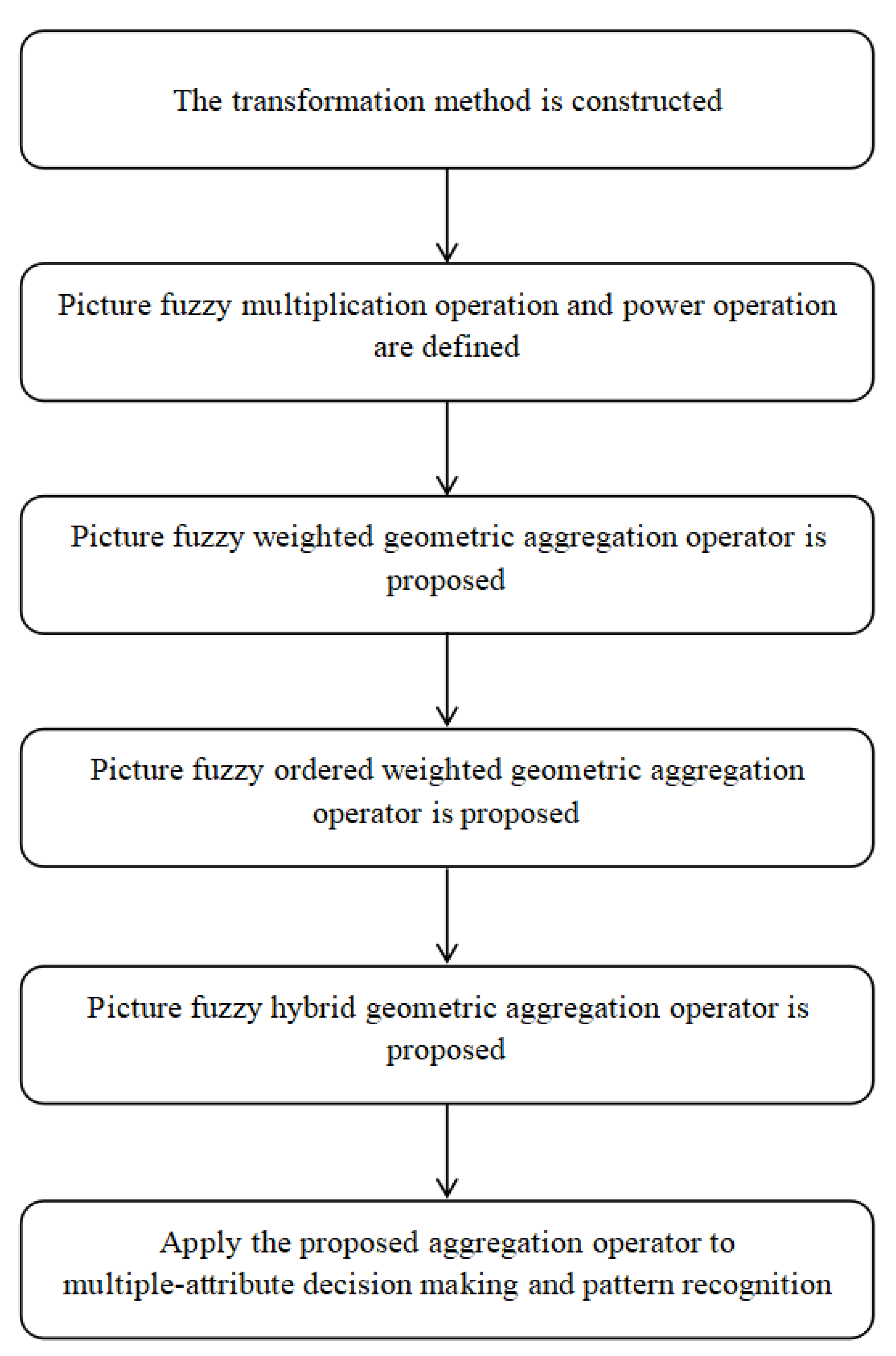
1.3. Main Contributions for This Paper

In order to overcome these defects, first, we construct the transformation method of picture fuzzy number and trapezoidal fuzzy number. Second, we define picture fuzzy multiplication operation and power operation. Third, we propose picture fuzzy weighted geometric aggregation operator, picture fuzzy ordered weighted geometric aggregation operator and picture fuzzy hybrid geometric aggregation operator and apply them to multi-attribute decision making problem. The research steps of this paper are shown in Figure 1.

The rest are organized as follows. In Section 2, we review basic concepts and properties for picture fuzzy sets. In Section 3, we present a transformation method for picture fuzzy number and trapezoid fuzzy number, based on this method, we proposed a multiplication operation and a power operation for picture fuzzy sets. In Section 4, we present three novel picture fuzzy aggregation operators based on the new multiplication operation and power operation. In Section 5, we discuss the efficiency and reasonable of the proposed aggregation operators by numerical cases, and applied the aggregation operators to multi-attribute decision making. In Section 6, we applied the aggregation operators to pattern recognition. The final section is conclusion.

2. Basic Concepts and Properties for Picture Fuzzy Sets

In this section, we review some basic concepts and properties for picture fuzzy sets, which will be used in this paper.

Definition 1

([2]). An intuitionistic fuzzy set (IFS) A on universe X is an object of the form:

$$A=\{\langle x,{\mu }_A(x),{\nu }_A(x)\rangle \mid x\in X\},$$

where ${\mu }_A(x)\in [0,1]$ is called “degree of membership" and ${\nu }_A(x)\in [0,1]$ is called “degree of non-membership", and where ${\mu }_A(x)$, ${\nu }_A(x)$ satisfies ${\mu }_A(x)+{\nu }_A(x)\le 1,\forall x\in X.$

Definition 2

([13]). A picture fuzzy set (PFS) A on universe X is an object of the form:

$$A=\{\langle x,{\mu }_A(x),{\eta }_A(x),{\nu }_A(x)\rangle \mid x\in X\},$$

where ${\mu }_A(x)\in [0,1]$ is called “degree of positive membership", ${\eta }_A(x)\in [0,1]$ is called “degree of neutral membership" and ${\nu }_A(x)\in [0,1]$ is called “degree of negative membership", and where ${\mu }_A(x)+{\eta }_A(x)+{\nu }_A(x)\le 1,\forall x\in X.$ For all $x\in X$, ${\rho }_A(x)=1-({\mu }_A(x)+{\eta }_A(x)+{\nu }_A(x))$ is called “degree of refusal membership".

We denote the family of all the picture fuzzy subsets on universe X by $PFS(X)$.

The set of all picture fuzzy numbers (PFNs) is denoted by $D^{*}=\{\alpha =\langle {\mu }_{\alpha },{\eta }_{\alpha },{\nu }_{\alpha }\rangle |\alpha \in {[0,1]}^3,{\mu }_{\alpha }+{\eta }_{\alpha }+{\nu }_{\alpha }\le 1\}$. For $\alpha =\langle {\mu }_{\alpha },{\eta }_{\alpha },{\nu }_{\alpha }\rangle ,\beta =\langle {\mu }_{\beta },{\eta }_{\beta },{\nu }_{\beta }\rangle \in D^{*}$, the order relation ${\le }_{D^{*}}$ is defined as $\alpha {\le }_{D^{*}}\beta$ if and only if ${\mu }_{\alpha }\le {\mu }_{\beta },$ and ${\mu }_{\alpha }+{\eta }_{\alpha }\le {\mu }_{\beta }+{\eta }_{\beta },$ and ${\nu }_{\alpha }\ge {\nu }_{\beta }$. $\alpha \vee \beta$ and $\alpha \wedge \beta$ are defined as follows [32]:

$$\begin{array}{cc}\hfill \alpha \vee \beta =& ({\mu }_{\alpha }\vee {\mu }_{\beta },({\mu }_{\alpha }+{\eta }_{\alpha })\vee ({\mu }_{\beta }+{\eta }_{\beta })-({\mu }_{\alpha }\vee {\mu }_{\beta }),{\nu }_{\alpha }\wedge {\nu }_{\beta }),\hfill \\ \hfill \alpha \wedge \beta =& ({\mu }_{\alpha }\wedge {\mu }_{\beta },({\mu }_{\alpha }+{\eta }_{\alpha })\wedge ({\mu }_{\beta }+{\eta }_{\beta })-({\mu }_{\alpha }\wedge {\mu }_{\beta }),{\nu }_{\alpha }\vee {\nu }_{\beta }).\hfill \end{array}$$

Then $(D^{*},{\le }_{D^{*}})$ is a complete lattice. The top element and bottom element are $1_{D^{*}}=(1,0,0)$ and $0_{D^{*}}=(0,0,1)$ on $D^{*}$, respectively.

Definition 3

([33]). Let $\tilde{a}=(a_1,a_2,a_3,a_4)$ be a trapezoidal fuzzy number, show in Figure 2. Its membership function ${\mu }_{\tilde{a}}(x)$ is defined as follows:

$${\mu }_{\tilde{a}}(x)=\left\{\begin{array}{cc}0\hfill & x<a_1,\hfill \\ \frac{x-a_1}{a_2-a_1}\hfill & a_1\le x\le a_2,\hfill \\ 1\hfill & a_2\le x\le a_3,\hfill \\ \frac{x-a_4}{a_3-a_4}\hfill & a_3\le x\le a_4,\hfill \\ 0\hfill & x>a_4.\hfill \end{array}\right.$$

If $a_1=a_2$, then $\tilde{a}$ is a right-angled trapezoid fuzzy number (show in Figure 3). The set of all the tight angled trapezoid fuzzy number is denoted by $C^{*}$, i.e., $C^{*}=\{\tilde{a}=(a_2,a_2,a_3,a_4)\}$.

Definition 4

([34]). Let $\tilde{a}=(a_1,a_2,a_3,a_4),\tilde{b}=(b_1,b_2,b_3,b_4)$ are two trapezoidal fuzzy numbers, the multiplication ⊙ is defined as $\tilde{a}\odot \tilde{b}=(a_1{b}_1,a_2{b}_2,a_3{b}_3,a_4{b}_4)$.

Proposition 1.

$C^{*}$ with respect to ⊙ is a Abel semigroup.

Definition 5.

A mapping $\mathcal{A}$: ${\cup }_{n\in N^{*}}$ $(D^{*}){}^n\to D^{*}$ is called an aggregation operator on $D^{*}$, if it satisfies the some properties:

(P1) $\mathcal{A}(\alpha )=\alpha (\forall \alpha \in D^{*})$;

(P2) Let ${\alpha }_j,{\beta }_j\in D^{*}$($j=1,2\dots ,n$), if ${\alpha }_j\le {\beta }_j(j=1,2,\dots ,n)$, then $\mathcal{A}({\alpha }_1,{\alpha }_2,\dots ,{\alpha }_n)\le \mathcal{A}({\beta }_1,{\beta }_2,\dots ,{\beta }_n)$;

(P3) $\mathcal{A}\left({\underbrace{0_{D^{*}},0_{D^{*}},\dots ,0_{D^{*}}}}_{ntims}\right)=0_{D^{*}}$;

(P4) $\mathcal{A}\left({\underbrace{1_{D^{*}},1_{D^{*}},\dots ,1_{D^{*}}}}_{ntims}\right)=1_{D^{*}}$.

Remark 1.

If the PFS reduces to the IFS, the Definition 5 is Definition 4.2 in [35].

Remark 2.

If the PFS reduces to the FS, the Definition 5 is Definition 2 in [36].

Definition 6

([31,37]). Let $\alpha =\langle {\mu }_{\alpha },{\eta }_{\alpha },{\nu }_{\alpha }\rangle \in D^{*}$, the score function S and accuracy function H of the picture fuzzy number are defined as follows:

$S(\alpha )={\mu }_{\alpha }-{\upsilon }_{\alpha },S(\alpha )\in [-1,1].$

$H(\alpha )={\mu }_{\alpha }+{\eta }_{\alpha }+{\upsilon }_{\alpha },H(\alpha )\in [0,1].$

Definition 7

([31]). Let $\alpha =\langle {\mu }_{\alpha },{\eta }_{\alpha },{\nu }_{\alpha }\rangle$ and $\beta =\langle {\mu }_{\beta },{\eta }_{\beta },{\nu }_{\beta }\rangle \in D^{*}$, if $S(\alpha )>S(\beta )$, then $\alpha >\beta ;$ if $S(\alpha )=S(\beta )$, then

(1) If $H(\alpha )>H(\beta )$, then $\alpha >\beta ;$

(2) If $H(\alpha )=H(\beta )$, then $\alpha =\beta .$

Let ${\alpha }_j=\langle {\mu }_{{\alpha }_j},{\eta }_{{\alpha }_j},{\nu }_{{\alpha }_j}\rangle (j=1,2,\dots ,n)\in D^{*}$. Some existing picture fuzzy weighted geometric ($PFWG$) aggregation operators, picture fuzzy ordered weighted geometric ($PFOWG$) aggregation operators and picture fuzzy hybrid geometric ($PFHG$) aggregation operators are shown in

Table 1. Some existing aggregation operators.

References	Aggregation Operators
Jana et al. [21]	$PFW{G}_1({\alpha }_1,{\alpha }_2,\dots ,{\alpha }_n)=\langle \frac{1}{1+{\{{\sum }_{j=1}^n{\omega }_j{(\frac{1-{\mu }_{{\alpha }_j}}{{\mu }_{{\alpha }_j}})}^{\xi }\}}^{\frac{1}{\xi }}},1-\frac{1}{1+{\{{\sum }_{j=1}^n{\omega }_j{(\frac{{\eta }_{{\alpha }_j}}{1-{\eta }_{{\alpha }_j}})}^{\xi }\}}^{\frac{1}{\xi }}},1-\frac{1}{1+{\{{\sum }_{j=1}^n{\omega }_j{(\frac{{\nu }_{{\alpha }_j}}{1-{\nu }_{{\alpha }_j}})}^{\xi }\}}^{\frac{1}{\xi }}}\rangle .$
	$PFOW{G}_1({\alpha }_1,{\alpha }_2,\dots ,{\alpha }_n)=\langle \frac{1}{1+{\{{\sum }_{j=1}^n{w}_j{(\frac{1-{\mu }_{{\alpha }_{\sigma (j)}}}{{\mu }_{{\alpha }_{\sigma (j)}}})}^{\xi }\}}^{\frac{1}{\xi }}},1-\frac{1}{1+{\{{\sum }_{j=1}^n{w}_j{(\frac{{\eta }_{{\alpha }_{\sigma (j)}}}{1-{\eta }_{{\alpha }_{\sigma (j)}}})}^{\xi }\}}^{\frac{1}{\xi }}},1-\frac{1}{1+{\{{\sum }_{j=1}^n{w}_j{(\frac{{\nu }_{{\alpha }_{\sigma (j)}}}{1-{\nu }_{{\alpha }_{\sigma (j)}}})}^{\xi }\}}^{\frac{1}{\xi }}}\rangle .$
	$PFH{G}_1({\alpha }_1,{\alpha }_2,\dots ,{\alpha }_n)=\langle \frac{1}{1+{\{{\sum }_{j=1}^n{W}_j{(\frac{1-{\mu }_{{\tilde{\alpha }}_{\sigma (j)}}}{{\mu }_{{\tilde{\alpha }}_{\sigma (j)}}})}^{\xi }\}}^{\frac{1}{\xi }}},1-\frac{1}{1+{\{{\sum }_{j=1}^n{W}_j{(\frac{{\eta }_{{\tilde{\alpha }}_{\sigma (j)}}}{1-{\eta }_{{\tilde{\alpha }}_{\sigma (j)}}})}^{\xi }\}}^{\frac{1}{\xi }}},1-\frac{1}{1+{\{{\sum }_{j=1}^n{W}_j{(\frac{{\nu }_{{\tilde{\alpha }}_{\sigma (j)}}}{1-{\nu }_{{\tilde{\alpha }}_{\sigma (j)}}})}^{\xi }\}}^{\frac{1}{\xi }}}\rangle .$
Wei [22]	$PFW{G}_2({\alpha }_1,{\alpha }_2,\dots ,{\alpha }_n)=\langle \frac{\gamma {\prod }_{j=1}^n{({\mu }_{{\alpha }_j})}^{{\omega }_j}}{{\prod }_{j=1}^n{[1+(\gamma -1)(1-{\mu }_{{\alpha }_j})]}^{{\omega }_j}+(\gamma -1){\prod }_{j=1}^n{({\mu }_{{\alpha }_j})}^{{\omega }_j}},$
	$\frac{{\prod }_{j=1}^n{[1+(\gamma -1){\eta }_{{\alpha }_j}]}^{{\omega }_j}-{\prod }_{j=1}^n{(1-{\eta }_{{\alpha }_j})}^{{\omega }_j}}{{\prod }_{j=1}^n{[1+(\gamma -1){\eta }_{{\alpha }_j}]}^{{\omega }_j}+(\gamma -1){\prod }_{j=1}^n{(1-{\eta }_{{\alpha }_j})}^{{\omega }_j}},$$\frac{{\prod }_{j=1}^n{[1+(\gamma -1){\nu }_{{\alpha }_j}]}^{{\omega }_j}-{\prod }_{j=1}^n{(1-{\nu }_{{\alpha }_j})}^{{\omega }_j}}{{\prod }_{j=1}^n{[1+(\gamma -1){\nu }_{{\alpha }_j}]}^{{\omega }_j}+(\gamma -1){\prod }_{j=1}^n{(1-{\nu }_{{\alpha }_j})}^{{\omega }_j}}\rangle .$
	$PFOW{G}_2({\alpha }_1,{\alpha }_2,\dots ,{\alpha }_n)=\langle \frac{\gamma {\prod }_{j=1}^n{({\mu }_{{\alpha }_{\sigma (j)}})}^{w_j}}{{\prod }_{j=1}^n{[1+(\gamma -1)(1-{\mu }_{{\alpha }_{\sigma (j)}})]}^{w_j}+(\gamma -1){\prod }_{j=1}^n{({\mu }_{{\alpha }_{\sigma (j)}})}^{w_j}},$
	$\frac{{\prod }_{j=1}^n{[1+(\gamma -1){\eta }_{{\alpha }_{\sigma (j)}}]}^{w_j}-{\prod }_{j=1}^n{(1-{\eta }_{{\alpha }_{\sigma (j)}})}^{w_j}}{{\prod }_{j=1}^n{[1+(\gamma -1){\eta }_{{\alpha }_{\sigma (j)}}]}^{w_j}+(\gamma -1){\prod }_{j=1}^n{(1-{\eta }_{{\alpha }_{\sigma (j)}})}^{w_j}},$$\frac{{\prod }_{j=1}^n{[1+(\gamma -1){\nu }_{{\alpha }_{\sigma (j)}}]}^{w_j}-{\prod }_{j=1}^n{(1-{\nu }_{{\alpha }_{\sigma (j)}})}^{w_j}}{{\prod }_{j=1}^n{[1+(\gamma -1){\nu }_{{\alpha }_{\sigma (j)}}]}^{w_j}+(\gamma -1){\prod }_{j=1}^n{(1-{\nu }_{{\alpha }_{\sigma (j)}})}^{w_j}}\rangle .$
	$PFH{G}_2({\alpha }_1,{\alpha }_2,\dots ,{\alpha }_n)=\langle \frac{\gamma {\prod }_{j=1}^n{({\mu }_{{\tilde{\alpha }}_{\sigma (j)}})}^{W_j}}{{\prod }_{j=1}^n{[1+(\gamma -1)(1-{\mu }_{{\tilde{\alpha }}_{\sigma (j)}})]}^{W_j}+(\gamma -1){\prod }_{j=1}^n{({\mu }_{{\tilde{\alpha }}_{\sigma (j)}})}^{W_j}},$
	$\frac{{\prod }_{j=1}^n{[1+(\gamma -1){\eta }_{{\tilde{\alpha }}_{\sigma (j)}}]}^{W_j}-{\prod }_{j=1}^n{(1-{\eta }_{{\tilde{\alpha }}_{\sigma (j)}})}^{W_j}}{{\prod }_{j=1}^n{[1+(\gamma -1){\eta }_{{\tilde{\alpha }}_{\sigma (j)}}]}^{W_j}+(\gamma -1){\prod }_{j=1}^n{(1-{\eta }_{{\tilde{\alpha }}_{\sigma (j)}})}^{W_j}},$$\frac{{\prod }_{j=1}^n{[1+(\gamma -1){\nu }_{{\tilde{\alpha }}_{\sigma (j)}}]}^{W_j}-{\prod }_{j=1}^n{(1-{\nu }_{{\tilde{\alpha }}_{\sigma (j)}})}^{W_j}}{{\prod }_{j=1}^n{[1+(\gamma -1){\nu }_{{\tilde{\alpha }}_{\sigma (j)}}]}^{W_j}+(\gamma -1){\prod }_{j=1}^n{(1-{\nu }_{{\tilde{\alpha }}_{\sigma (j)}})}^{W_j}}\rangle .$
Ashraf et al. [25]	$PFW{G}_3({\alpha }_1,{\alpha }_2,\dots ,{\alpha }_n)=\langle {\prod }_{j=1}^n{({\mu }_{{\alpha }_j})}^{{\omega }_j},{\prod }_{j=1}^n{({\eta }_{{\alpha }_j})}^{{\omega }_j},1-{\prod }_{j=1}^n(1-{{\nu }_{{\alpha }_j})}^{{\omega }_j}\rangle .$
	$PFOW{G}_3({\alpha }_1,{\alpha }_2,\dots ,{\alpha }_n)=\langle {\prod }_{j=1}^n{({\mu }_{{\alpha }_{\sigma (j)}})}^{w_j},{\prod }_{j=1}^n{({\eta }_{{\alpha }_{\sigma (j)}})}^{w_j},1-{\prod }_{j=1}^n(1-{{\nu }_{{\alpha }_{\sigma (j)}})}^{w_j}\rangle .$
	$PFH{G}_3({\alpha }_1,{\alpha }_2,\dots ,{\alpha }_n)=\langle {\prod }_{j=1}^n{({\mu }_{{\tilde{\alpha }}_{\sigma (j)}})}^{W_j},{\prod }_{j=1}^n{({\eta }_{{\tilde{\alpha }}_{\sigma (j)}})}^{W_j},1-{\prod }_{j=1}^n(1-{{\nu }_{{\tilde{\alpha }}_{\sigma (j)}})}^{W_j}\rangle .$
Wang et al. [26]	$PFW{G}_4({\alpha }_1,{\alpha }_2,\dots ,{\alpha }_n)=\langle {\prod }_{j=1}^n{({\mu }_{{\alpha }_j}+{\eta }_{{\alpha }_j})}^{{\omega }_j}-{\prod }_{j=1}^n{({\eta }_{{\alpha }_j})}^{{\omega }_j},{\prod }_{j=1}^n{({\eta }_{{\alpha }_j})}^{{\omega }_j},1-{\prod }_{j=1}^n(1-{{\nu }_{{\alpha }_j})}^{{\omega }_j}\rangle .$
	$PFOW{G}_4({\alpha }_1,{\alpha }_2,\dots ,{\alpha }_n)=\langle {\prod }_{j=1}^n{({\mu }_{{\alpha }_{\sigma (j)}}+{\eta }_{{\alpha }_{\sigma (j)}})}^{w_j}-{\prod }_{j=1}^n{({\eta }_{{\alpha }_{\sigma (j)}})}^{w_j},{\prod }_{j=1}^n{({\eta }_{{\alpha }_{\sigma (j)}})}^{w_j},1-{\prod }_{j=1}^n(1-{{\nu }_{{\alpha }_{\sigma (j)}})}^{w_j}\rangle .$
	$PFH{G}_4({\alpha }_1,{\alpha }_2,\dots ,{\alpha }_n)=\langle {\prod }_{j=1}^n{({\mu }_{{\tilde{\alpha }}_{\sigma (j)}}+{\eta }_{{\tilde{\alpha }}_{\sigma (j)}})}^{W_j}-{\prod }_{j=1}^n{({\eta }_{{\tilde{\alpha }}_{\sigma (j)}})}^{W_j},{\prod }_{j=1}^n{({\eta }_{{\tilde{\alpha }}_{\sigma (j)}})}^{W_j},1-{\prod }_{j=1}^n(1-{{\nu }_{{\tilde{\alpha }}_{\sigma (j)}})}^{W_j}\rangle .$
Wei [31]	$PFW{G}_5({\alpha }_1,{\alpha }_2,\dots ,{\alpha }_n)=\langle {\prod }_{j=1}^n{({\mu }_{{\alpha }_j})}^{{\omega }_j},1-{\prod }_{j=1}^n{(1-{\eta }_{{\alpha }_j})}^{{\omega }_j},1-{\prod }_{j=1}^n{(1-{\nu }_{{\alpha }_j})}^{{\omega }_j}\rangle .$
	$PFOW{G}_5({\alpha }_1,{\alpha }_2,\dots ,{\alpha }_n)=\langle {\prod }_{j=1}^n{({\mu }_{{\alpha }_{\sigma (j)}})}^{w_j},1-{\prod }_{j=1}^n{(1-{\eta }_{{\alpha }_{\sigma (j)}})}^{w_j},1-{\prod }_{j=1}^n{(1-{\nu }_{{\alpha }_{\sigma (j)}})}^{w_j}\rangle .$
	$PFH{G}_5({\alpha }_1,{\alpha }_2,\dots ,{\alpha }_n)=\langle {\prod }_{j=1}^n{({\mu }_{{\tilde{\alpha }}_{\sigma (j)}})}^{W_j},1-{\prod }_{j=1}^n{(1-{\eta }_{{\tilde{\alpha }}_{\sigma (j)}})}^{W_j},1-{\prod }_{j=1}^n{(1-{\nu }_{{\tilde{\alpha }}_{\sigma (j)}})}^{W_j}\rangle .$

.

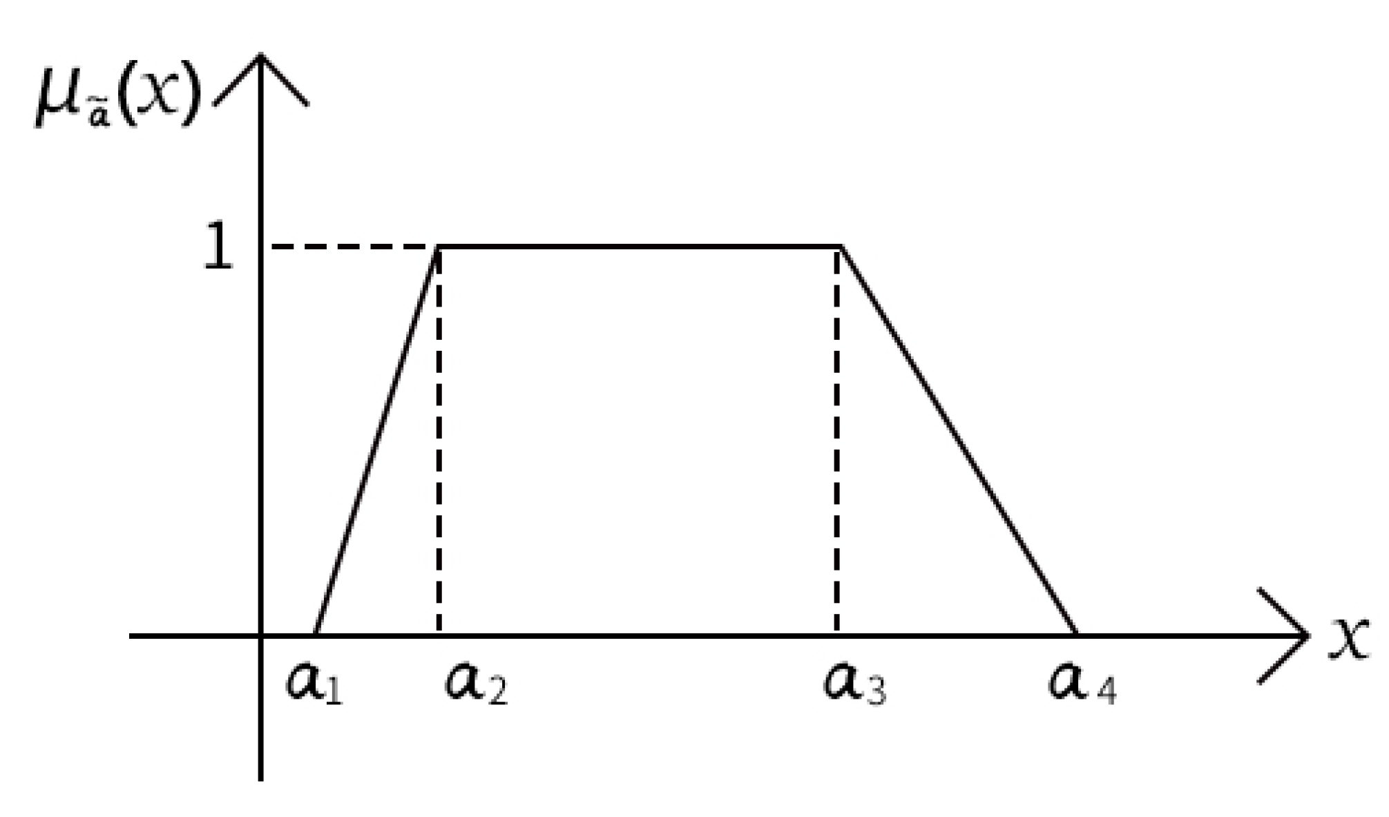
3. New Transformation Approach for Picture Fuzzy Sets

In this section, we introduce a transformation method between picture fuzzy numbers and trapezoidal fuzzy numbers.

Proposition 2.

Let $\alpha =\langle {\mu }_{\alpha },{\eta }_{\alpha },{\nu }_{\alpha }\rangle ,\beta =\langle {\mu }_{\beta },{\eta }_{\beta },{\nu }_{\beta }\rangle \in D^{*},\otimes :{(D^{*})}^2\to D^{*}$ is defined as $\alpha \otimes \beta =\langle 1-(1-{\mu }_{\alpha })(1-{\mu }_{\beta }),(1-{\mu }_{\alpha })(1-{\mu }_{\beta })-(1-{\mu }_{\alpha }-{\eta }_{\alpha })(1-{\mu }_{\beta }-{\eta }_{\beta }),(1-{\mu }_{\alpha }-{\eta }_{\alpha })(1-{\mu }_{\beta }-{\eta }_{\beta })-(1-{\mu }_{\alpha }-{\eta }_{\alpha }-{\nu }_{\alpha })(1-{\mu }_{\beta }-{\eta }_{\beta }-{\nu }_{\beta })\rangle ,$ then $(D^{*},\otimes )$ is a Abel semigroup.

Definition 8.

Let $\alpha =\langle {\mu }_{\alpha },{\eta }_{\alpha },{\nu }_{\alpha }\rangle \in D^{*}$, $\lambda \in [0,1]$. The power operation is ${\alpha }^{\lambda }=〈1-{(1-{\mu }_{\alpha })}^{\lambda },{(1-{\mu }_{\alpha })}^{\lambda }-{(1-{\mu }_{\alpha }-{\eta }_{\alpha })}^{\lambda },{(1-{\mu }_{\alpha }-{\eta }_{\alpha })}^{\lambda }-{(1-{\mu }_{\alpha }-{\eta }_{\alpha }-{\nu }_{\alpha })}^{\lambda }〉.$

Theorem 1.

Semigroup $D^{*}$ is isomorphic to semigroup $C^{*}$.

4. New Geometric Aggregation Operators for Picture Fuzzy Sets

In this section, we introduce the picture fuzzy weighted geometric ($PFWG$) aggregation operator, the picture fuzzy ordered weighted geometric ($PFOWG$) aggregation operator and the picture fuzzy hybrid geometric ($PFHG$) aggregation operator based on the picture fuzzy multiplication operation and the picture fuzzy power operation.

Theorem 2.

Let ${\alpha }_j=\langle {\mu }_{{\alpha }_j},{\eta }_{{\alpha }_j},{\nu }_{{\alpha }_j}\rangle (j=1,2,\dots ,n)\in D^{*}$, a mapping $PFWG$: ${\cup }_{n\in N^{*}}$ ${(D^{*})}^n\to D^{*}$ is defined as follow:

$$\begin{array}{cc}\hfill PFWG({\alpha }_1,{\alpha }_2,\dots ,{\alpha }_n)=& {\alpha }_1^{{\omega }_1}\otimes {\alpha }_2^{{\omega }_2}\otimes \dots \otimes {\alpha }_n^{{\omega }_n}\hfill \\ \hfill =& \langle 1-\prod _{j=1}^n{(1-{\mu }_{{\alpha }_j})}^{{\omega }_j},\prod _{j=1}^n{(1-{\mu }_{{\alpha }_j})}^{{\omega }_j}-\prod _{j=1}^n{(1-{\mu }_{{\alpha }_j}-{\eta }_{{\alpha }_j})}^{{\omega }_j},\hfill \\ \hfill & \prod _{j=1}^n{(1-{\mu }_{{\alpha }_j}-{\eta }_{{\alpha }_j})}^{{\omega }_j}-\prod _{j=1}^n{(1-{\mu }_{{\alpha }_j}-{\eta }_{{\alpha }_j}-{\nu }_{{\alpha }_j})}^{{\omega }_j}\rangle .\hfill \end{array}$$

(1)

where $\omega =({\omega }_1,{\omega }_2,\dots ,{\omega }_n)$ is the weighting vector of ${\alpha }_j(j=1,2,\dots ,n)$, with ${\omega }_j\in [0,1]$ and ${\sum }_{j=1}^n{\omega }_j=1$. Then the mapping $PFWG$ is an aggregation operator, and called picture fuzzy weighted geometric ($PFWG$) aggregation operator.

Remark 3.

If $\omega =(\frac{1}{n},\frac{1}{n},\frac{1}{n},\dots ,\frac{1}{n})$, then $PFWG$ is called the picture fuzzy geometric average aggregation operator:

$$\begin{array}{cc}\hfill PFWG({\alpha }_1,{\alpha }_2,\dots ,{\alpha }_n)=& \langle 1-\prod _{j=1}^n{(1-{\mu }_{{\alpha }_j})}^{\frac{1}{n}},\prod _{j=1}^n{(1-{\mu }_{{\alpha }_j})}^{\frac{1}{n}}-\prod _{j=1}^n{(1-{\mu }_{{\alpha }_j}-{\eta }_{{\alpha }_j})}^{\frac{1}{n}},\hfill \\ \hfill & \prod _{j=1}^n{(1-{\mu }_{{\alpha }_j}-{\eta }_{{\alpha }_j})}^{\frac{1}{n}}-\prod _{j=1}^n{(1-{\mu }_{{\alpha }_j}-{\eta }_{{\alpha }_j}-{\nu }_{{\alpha }_j})}^{\frac{1}{n}}\rangle .\hfill \end{array}$$

Theorem 3.

Let ${\alpha }_j=\langle {\mu }_{{\alpha }_j},{\eta }_{{\alpha }_j},{\nu }_{{\alpha }_j}\rangle (j=1,2,\dots ,n)\in D^{*}$, a mapping $PFOWG$: ${\cup }_{n\in N^{*}}$ ${(D^{*})}^n\to D^{*}$ is defined as follow:

$$\begin{array}{cc}\hfill PFOWG({\alpha }_1,{\alpha }_2,\dots ,{\alpha }_n)=& {\alpha }_{\sigma (1)}^{w_1}\otimes {\alpha }_{\sigma (2)}^{w_2}\otimes \dots \otimes {\alpha }_{\sigma (n)}^{w_n}\hfill \\ \hfill =& \langle 1-\prod _{j=1}^n{(1-{\mu }_{{\alpha }_{\sigma (j)}})}^{w_j},\prod _{j=1}^n{(1-{\mu }_{{\alpha }_{\sigma (j)}})}^{w_j}-\prod _{j=1}^n{(1-{\mu }_{{\alpha }_{\sigma (j)}}-{\eta }_{{\alpha }_{\sigma (j)}})}^{w_j},\hfill \\ & \prod _{j=1}^n{(1-{\mu }_{{\alpha }_{\sigma (j)}}-{\eta }_{{\alpha }_{\sigma (j)}})}^{w_j}-\prod _{j=1}^n{(1-{\mu }_{{\alpha }_{\sigma (j)}}-{\eta }_{{\alpha }_{\sigma (j)}}-{\nu }_{{\alpha }_{\sigma (j)}})}^{w_j}\rangle .\hfill \end{array}$$

(2)

where $\sigma (j)$ is a permutation of $(1,2,\dots ,n)$, i.e., ${\alpha }_{\sigma (j-1)}\ge {\alpha }_{{\sigma }_{(j)}}$ $j=(1,2,\dots ,n)$, ${\alpha }_{{\sigma }_j}$ is the jth largest of ${\alpha }_j$ in descending order. $w=(w_1,w_2,\dots ,w_n)$ is the weighting vector of $PFOWG$, with $w_j\in [0,1]$ and ${\sum }_{j=1}^n{w}_j=1$. Then the mapping $PFOWG$ is an aggregation operator, and called picture fuzzy ordered weighted geometric ($PFOWG$) aggregation operator.

Theorem 4.

Let ${\alpha }_j=\langle {\mu }_{{\alpha }_j},{\eta }_{{\alpha }_j},{\nu }_{{\alpha }_j}\rangle (j=1,2,\dots ,n)\in D^{*}$, a mapping $PFHG$: ${\cup }_{n\in N^{*}}$ ${(D^{*})}^n\to D^{*}$ is defined as follow:

$$\begin{array}{cc}\hfill PFHG({\alpha }_1,{\alpha }_2,\dots ,{\alpha }_n)=& {\tilde{\alpha }}_{\sigma (1)}^{W_1}\otimes {\tilde{\alpha }}_{\sigma (2)}^{W_2}\otimes \dots \otimes {\tilde{\alpha }}_{\sigma (n)}^{W_n}\hfill \\ \hfill =& \langle 1-\prod _{j=1}^n{(1-{\mu }_{{\tilde{\alpha }}_{\sigma (j)}})}^{W_j},\prod _{j=1}^n{(1-{\mu }_{{\tilde{\alpha }}_{\sigma (j)}})}^{W_j}-\prod _{j=1}^n{(1-{\mu }_{{\tilde{\alpha }}_{\sigma (j)}}-{\eta }_{{\tilde{\alpha }}_{\sigma (j)}})}^{W_j},\hfill \\ & \prod _{j=1}^n{(1-{\mu }_{{\tilde{\alpha }}_{\sigma (j)}}-{\eta }_{{\tilde{\alpha }}_{\sigma (j)}})}^{W_j}-\prod _{j=1}^n{(1-{\mu }_{{\tilde{\alpha }}_{\sigma (j)}}-{\eta }_{{\tilde{\alpha }}_{\sigma (j)}}-{\nu }_{{\tilde{\alpha }}_{\sigma (j)}})}^{W_j}\rangle .\hfill \end{array}$$

(3)

where $\sigma (j)$ is a permutation of $(1,2,\dots ,n)$, i.e., ${\alpha }_{\sigma (j-1)}\ge {\alpha }_{{\sigma }_{(j)}}$ $j=(1,2,\dots ,n)$. ${\tilde{\alpha }}_j={\alpha }_j^{n{\omega }_j}(j=1,2,\dots ,n)$ is weighted ${\alpha }_j$, n is the number of ${\alpha }_j$, ${\omega }_j=({\omega }_1,{\omega }_2,\dots ,{\omega }_n)(j=1,2,\dots n)$ is the weighting vector of ${\alpha }_j$, with ${\omega }_j\in [0,1]$ and ${\sum }_{j=1}^n{\omega }_j=1$. ${\tilde{\alpha }}_{\sigma (j)}$ is jth largest of ${\tilde{\alpha }}_j$ in descending order. $W_j=(W_1,W_2,\dots ,W_n)(j=1,2,\dots n)$ is the weighting vector of $PFHG$, with $W_j\in [0,1]$ and ${\sum }_{j=1}^n{W}_j=1$. Then the mapping $PFHG$ is an aggregation operator, and called picture fuzzy hybrid geometric ($PFHG$) aggregation operator.

Remark 4.

If the PFS reduces to the IFS, the $PFWG$ aggregation operator reduces to $IFWG$ aggregation operator; the $PFOWG$ aggregation operator reduces to $IFOWG$ aggregation operator; $PFHG$ aggregation operator reduces to $IFHG$ aggregation operator. These aggregation operators of intuitionistic fuzzy can be found in [38].

5. Application to Multi-Criteria Decision Making

In this section, to demonstrate the effectiveness of the proposed aggregation operators, we use numerical example to compare with some existing aggregation operators. To demonstrate the practicability of the proposed aggregation operators, we give the algorithm for the multi-attribute decision making, and apply the proposed three aggregation operators to solve the multi-attribute decision making.

5.1. Numerical Example

Example 1.

Let ${\alpha }_1=\langle 0.1,0.0,0.2\rangle$, ${\alpha }_2=\langle 0.2,0.1,0.0\rangle$, ${\alpha }_3=\langle 0.0,0.1,0.2\rangle$ and ${\alpha }_4=\langle 0.3,0.3,0.1\rangle$ are four PFNs, the weighting vector of ${\alpha }_j(j=1,2,3,4)$ is $\omega =(0.25,0.25,0.25,0.25)$. Assume that the weighting vector of $PFOWG$ aggregation operator is $w=(0.25,0.25,0.25,0.25)$, the weighting vector of $PFHG$ aggregation operator is $W=(0.25,0.25,0.25,0.25)$. Based on the $PFWG$, $PFOWG$ and $PFHG$ aggregation operators of some existing and proposed, the results of aggregation are shown in

Table 2. Results of aggregation.

	PFWG	PFOWG	PFHG
Jana et al. [21] ($\xi =1$)	Cannot be calculated	Cannot be calculated	Cannot be calculated
Wei [22] ($\gamma =2$)	$\langle \mathbf{0.0000},0.1269,0.1258\rangle$	$\langle \mathbf{0.0000},0.1269,0.1258\rangle$	$\langle \mathbf{0.0000},0.1269,0.1258\rangle$
Ashraf et al. [25]	$\langle \mathbf{0.0000},\mathbf{0.0000},0.1288\rangle$	$\langle \mathbf{0.0000},\mathbf{0.0000},0.1288\rangle$	$\langle \mathbf{0.0000},\mathbf{0.0000},0.1288\rangle$
Wang et al. [26]	$\langle 0.2060,\mathbf{0.0000},0.1288\rangle$	$\langle 0.2060,\mathbf{0.0000},0.1288\rangle$	$\langle 0.2060,\mathbf{0.0000},0.1288\rangle$
Wei [31]	$\langle \mathbf{0.0000},0.1322,0.1288\rangle$	$\langle \mathbf{0.0000},0.1322,0.1288\rangle$	$\langle \mathbf{0.0000},0.1322,0.1288\rangle$
The proposed	$\langle 0.1574,0.1525,0.1237\rangle$	$\langle 0.1574,0.1525,0.1237\rangle$	$\langle 0.1574,0.1525,0.1237\rangle$

.

From Table 2, we can see that some existing aggregation operators have drawbacks. Wei [22], Ashraf et al. [25] and Wei [31]’ positive membership degree of aggregate result is zero, though n − 1 positive membership degree are not equal to zero. Wang et al. [26]’ neutral membership degree of aggregate result is zero, though n − 1 neutral membership degree are not equal to zero. Moreover, Jana et al. [21] aggregation operators cannot be calculated, because the zero in the denominator. However, the proposed aggregation operators overcome this defect, positive membership degree and neutral membership degree of aggregate results are not equal to zero. Therefore, the proposed aggregation operators are more effective.

5.2. Application to Multi-Criteria Decision Making

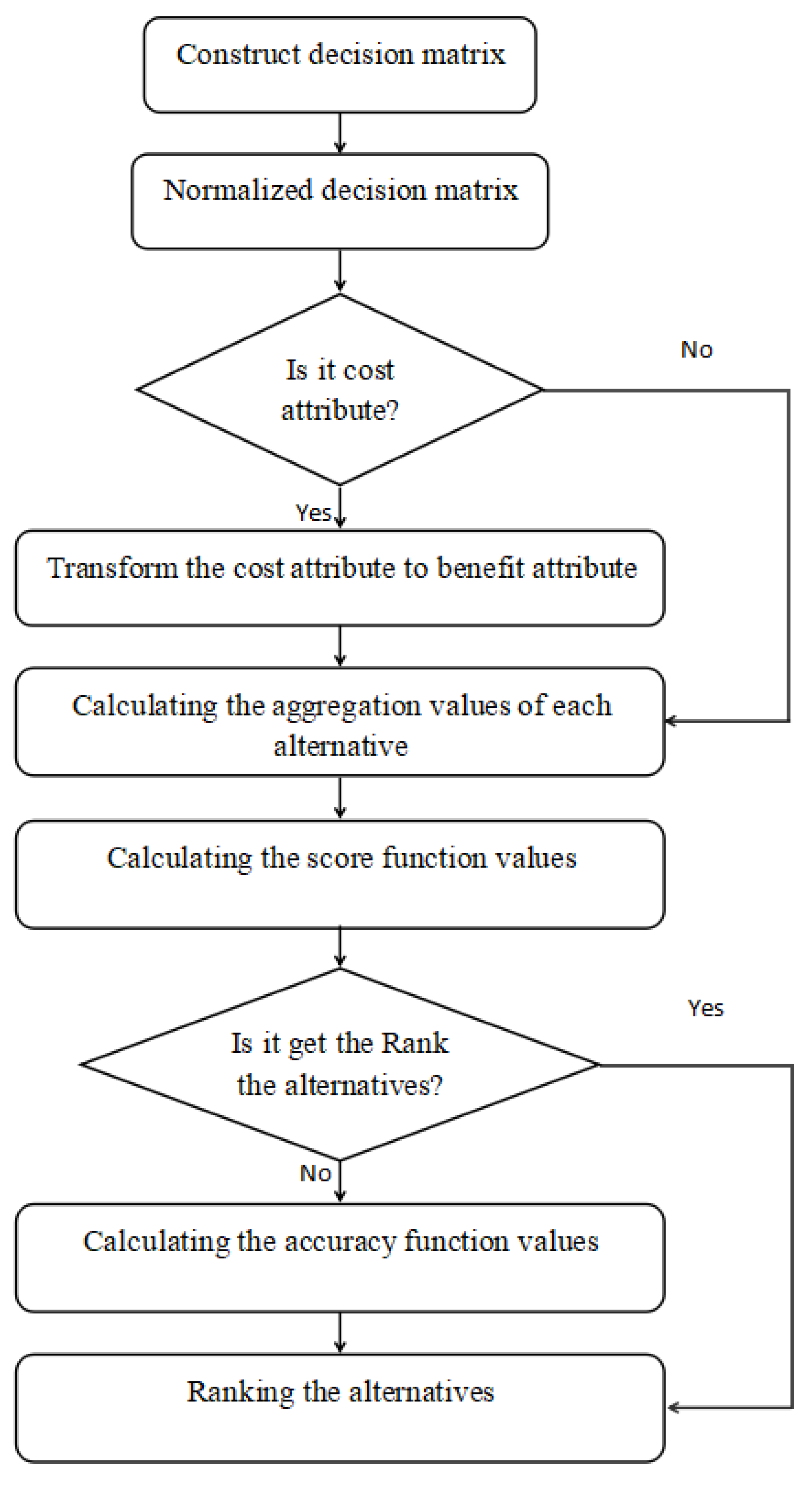
5.2.1. Algorithm for Multi-Criteria Decision Making

Suppose, there’s m alternatives, which denoted by $A=\{A_1,A_2,\dots ,A_m\}$. The alternatives have been evaluated by the PFNs under the set of attribute $C=\{C_1,C_2,\dots ,C_n\}$. The weighting vector of attribute is $\omega =({\omega }_1,{\omega }_2,\dots ,{\omega }_n)$, and ${\omega }_j\in [0,1]$, ${\sum }_{i=1}^n{\omega }_j=1$. Construct decision matrix $D={({\alpha }_{ij})}_{m\times n}$. Which is the best alternative?

A new multi-attribute decision making algorithm is shown in Figure 4.

Step 1: Normalized decision matrix:

$$r_{ij}=\left\{\begin{array}{c}\hfill {\alpha }_{ij}^c,\mathrm{for}\cos \mathrm{t}\mathrm{attribute}{C}_j\\ \hfill {\alpha }_{ij},\mathrm{for}\mathrm{benefit}\mathrm{attribute}{C}_j\end{array}\right.$$

where ${\alpha }_{ij}^c=\langle {\nu }_{ij},{\eta }_{ij},{\mu }_{ij}\rangle$ is the complement of ${\alpha }_{ij}=\langle {\mu }_{ij},{\eta }_{ij},{\nu }_{ij}\rangle$.

Step 2: Calculating the aggregation values of each alternative $A_i(i=1,2,\dots ,m)$ by using the aggregation operator $PFWG$(or $PFOWG$, or $PFHG$).

Step 3: Calculating the score function values $S(A_i)$ of aggregation alternative by Definition 6.

Step 4: Ranking the alternatives by Definition 7, the greatest score value is the best alternative.

5.2.2. Application to Multi-Criteria Decision Making

Example 2.

Suppose an investment firm wants to choose a corporation to invest in. According to market research, there are three possible alternatives, which are denoted by $A=\{A_1,A_2,A_3\}$: mobile phone corporation $A_1$, television corporation $A_2$, computer corporation $A_3$. There are five attributes $C=\{C_1,C_2,C_3,C_4,C_5\}$: resources analysis $(C_1)$, economy analysis $(C_2)$, market analysis $(C_3)$, environmental analysis $(C_4)$, infrastructure analysis $(C_5)$, are considered. The weighting vector of the five attributes is $\omega =(0.2,0.3,0.1,0.1,0.3)$. The three possible alternatives be evaluated by the PFNs under the five attributes. The decision matrix constructed is shown in

Table 3. Picture fuzzy decision matrix.

	${\mathit{C}}_1$	${\mathit{C}}_2$	${\mathit{C}}_3$	${\mathit{C}}_4$	${\mathit{C}}_5$
$A_1$	$\langle 0.1,0.2,0.1\rangle$	$\langle 0.4,0.3,0.2\rangle$	$\langle 0.0,0.0,1.0\rangle$	$\langle 0.2,0.2,0.1\rangle$	$\langle 0.2,0.1,0.4\rangle$
$A_2$	$\langle 0.2,0.0,0.7\rangle$	$\langle 0.4,0.1,0.1\rangle$	$\langle 0.1,0.5,0.0\rangle$	$\langle 0.3,0.2,0.4\rangle$	$\langle 0.0,0.0,1.0\rangle$
$A_3$	$\langle 0.3,0.1,0.6\rangle$	$\langle 0.0,0.0,1.0\rangle$	$\langle 0.2,0.4,0.0\rangle$	$\langle 0.1,0.4,0.1\rangle$	$\langle 0.4,0.1,0.4\rangle$

. Which company should the investment company choose to invest?

We use the $PFWG,PFOWG$ and $PFHG$ aggregation operators to calculate, respectively. As follows:

(i) Using proposed $PFWG$ aggregation operator.

Step 1: Since the five attributes are all benefit attributes, the picture fuzzy decision matrix is normalized decision matrix.

Step 2: Calculating the aggregation values of each alternative by using the proposed $PFWG$ aggregation operator, we have

$$A_1:\langle 0.2317,0.2143,0.5540\rangle ,A_2:\langle 0.2166,0.1221,0.6613\rangle ,A_3:\langle 0.2270,0.1487,0.6243\rangle .$$

Step 3: Calculating the score function values of each aggregation alternative by Definition 6, we have

$$S(A_1)=-0.3223,S(A_2)=-0.4447,S(A_3)=-0.3973.$$

Step 4: Ranking the alternatives by Definition 7, the greatest score value is the best alternative. We have $S(A_1)>S(A_3)>S(A_2)$. Therefore

$$A_1>A_3>A_2.$$

The best alternative is $A_1$, i.e., to invest the mobile phone company.

(ii) Using proposed $PFOWG$ aggregation operator.

Step 1: Since the five attributes are all benefit attributes, the picture fuzzy decision matrix is the normalized decision matrix.

First, calculating the score values of each criteria according to the Definition 6 and rank the criteria in order of the highest score values to the lowest, the picture fuzzy ordered decision matrix in

Table 4. Picture fuzzy ordered decision matrix.

	${\mathit{C}}_1$	${\mathit{C}}_2$	${\mathit{C}}_3$	${\mathit{C}}_4$	${\mathit{C}}_5$
$A_{{\sigma }_1}$	$\langle 0.4,0.3,0.2\rangle$	$\langle 0.2,0.2,0.1\rangle$	$\langle 0.1,0.2,0.1\rangle$	$\langle 0.2,0.1,0.5\rangle$	$\langle 0.0,0.0,1.0\rangle$
$A_{{\sigma }_2}$	$\langle 0.4,0.1,0.1\rangle$	$\langle 0.1,0.5,0.0\rangle$	$\langle 0.3,0.2,0.4\rangle$	$\langle 0.2,0.0,0.7\rangle$	$\langle 0.0,0.0,1.0\rangle$
$A_{{\sigma }_3}$	$\langle 0.2,0.4,0.0\rangle$	$\langle 0.4,0.1,0.4\rangle$	$\langle 0.1,0.4,0.1\rangle$	$\langle 0.3,0.1,0.6\rangle$	$\langle 0.0,0.0,1.0\rangle$

.

Step 2: Calculating the aggregation values by using the proposed $PFOWG$ aggregation operator, where the weighting vector of $PFOWG$ aggregation operator is $w=(0.2,0.3,0.1,0.1,0.3)$, we have

$$A_1:\langle 0.1829,0.1892,0.6279\rangle ,A_2:\langle 0.1745,0.2221,0.6034\rangle ,A_3:\langle 0.2166,0.1839,0.5995\rangle .$$

Step 3: Calculating the score function values of each aggregation alternative by Definition 6, we have

$$S_1=-0.4450,S_2=-0.4289,S_3=-0.3829.$$

Step 4: Ranking the alternatives by Definition 7, the greatest score value is the best alternative. We have $S(A_3)>S(A_2)>S(A_1)$. Therefore

$$A_3>A_2>A_1.$$

The best alternative is $A_3$, i.e., to invest the computer company.

(iii) Using proposed $PFHG$ aggregation operator.

Step 1: Since the five attributes are all benefit attributes, the picture fuzzy decision matrix is the normalized decision matrix.

First, aggregation the evaluating PFNs of alternatives by using the proposed multiplication operation and power operation, ${\tilde{A}}_{ij}=A_{ij}^{n\omega }(i=1,2,3;j=1,2,3,4,5)$, where $\omega =(0.2,0.3,0.1,0.1,0.3)$ is weighting vector of $A_{i1},A_{i2},A_{i3},A_{i4},A_{i5}$ and n = 5. Then, calculating the score values of aggregation evaluating PFNs by Definition 6 and rank the criteria according to the Definition 7, the picture fuzzy ordered weighted decision matrix in

Table 5. Picture fuzzy ordered weighted decision matrix.

	${\tilde{\mathit{A}}}_{{\mathit{\sigma }}_1}$	${\tilde{\mathit{A}}}_{{\mathit{\sigma }}_2}$	${\tilde{\mathit{A}}}_{{\mathit{\sigma }}_3}$
$C_1$	$\langle 0.5352,0.3005,0.1327\rangle$	$\langle 0.5352,0.1112,0.1006\rangle$	$\langle 0.5352,0.1112,0.3219\rangle$
$C_2$	$\langle 0.1056,0.1198,0.0675\rangle$	$\langle 0.0513,0.3162,0.0000\rangle$	$\langle 0.1056,0.2620,0.0000\rangle$
$C_3$	$\langle 0.1000,0.2000,0.1000\rangle$	$\langle 0.1633,0.1296,0.3909\rangle$	$\langle 0.0513,0.2416,0.0747\rangle$
$C_4$	$\langle 0.2845,0.1298,0.4214\rangle$	$\langle 0.2000,0.0000,0.7000\rangle$	$\langle 0.3000,0.1000,0.6000\rangle$
$C_5$	$\langle 0.0000,0.0000,1.0000\rangle$	$\langle 0.0000,0.0000,1.0000\rangle$	$\langle 0.0000,0.0000,1.0000\rangle$

.

Step 2: Calculating the aggregation values of each alternative by using the proposed $PFHG$ aggregation operator. Where the weighting vector of $PFHG$ aggregation operator is $W=(0.112,0.236,0.304,0.236,0.112)$ based on the normal distribution in [39], we have

$$A_1:\langle 0.2000,0.1918,0.6082\rangle ,A_2:\langle 0.1854,0.1325,0.6821\rangle ,A_3:\langle 0.1913,0.1714,0.6373\rangle .$$

Step 3: Calculating the score function values of each aggregation alternative according to the Definition 6, we can get

$$S(A_1)=-0.4082,S(A_2)=-0.4967,S(A_3)=-0.4460.$$

Step 4: Ranking the alternatives according to the Definition 7, the greatest score value is the best alternative. We have $S(A_1)>S(A_3)>S(A_2)$. Therefore

$$A_1>A_3>A_2.$$

The best alternative is $A_1$, i.e., to invest the mobile phone company.

(iv) Compare analysis with some existing aggregation operators, the results are summarized in

Table 6. Comparison analysis results.

References	PFWG	PFOWG	PFHG
Jana et al. [21]	Cannot be calculated	Cannot be calculated	Cannot be calculated
Wei [22]	$A_1=A_2=A_3$	$A_1=A_2=A_3$	$A_1=A_2=A_3$
Ashraf et al. [25]	$A_1=A_2=A_3$	$A_1=A_2=A_3$	$A_1=A_2=A_3$
Wang et al. [26]	$A_1=A_2=A_3$	$A_1=A_2=A_3$	$A_1=A_2=A_3$
Wei [31]	$A_1=A_2=A_3$	$A_1=A_2=A_3$	$A_1=A_2=A_3$
The proposed operator	$A_1>A_3>A_2$	$A_3>A_2>A_1$	$A_1>A_3>A_2$

.

The best alternative are $A_1$ by using the proposed $PFWG$ and $PFHG$ aggregation operators. i.e., to invest the mobile phone company. By using the $PFOWG$ aggregation operator, we can get $A_3>A_2>A_1$, the best alternative is $A_3$, i.e., to invest the computer company. These three operators $PFWG$, $PFOWG$ and $PFHG$ provide different choices for decision makers. Decision makers can choose $PFWG$ aggregation operator when only consider the self importance of each criteria. Decision makers can choose $PFOWG$ aggregation operator when only consider the ordered position importance of each criteria. Decision makers can choose $PFHG$ aggregation operator when both consider the self importance and the ordered position importance of each criteria.

From Table 6, we can see that by using the aggregation operators in [22,25,26,31], the decision results are $A_1=A_2=A_3$, which cannot rank for alternative $A_1$, $A_2$ and $A_3$. The aggregation operators of [21] cannot calculate the result of aggregation because the denominator appears 0 in the calculation process. However, the proposed aggregation operators can overcome this defect and obtain rank of the alternatives. Therefore, we proposed aggregation operators are not only effective, but also overcome the shortcomings of some aggregation operators.

Example 3

([31]). One team plans to implement an enterprise resource planning (ERP) system. The first is to build a project team. Project term choose five potential ERP systems $A_i(i=1,2,\dots ,5)$ are to be evaluated by the PFNs under the four attributes $C_1$: function and technology, $C_2$ strategic fitness, $C_3$: vendor’s ability, $C_4$: vendor’s reputation, whose weighting vector is $\omega =(0.2,0.1,0.3,0.4)$. Suppose that the weighting vector of $PFOWG$ aggregation operator is $w=(0.2,0.1,0.3,0.4)$, the weighting vector of $PFHG$ aggregation operator is $W=(0.140,0.264,0.332,0.264)$, and construct the following matrix is shown in

Table 7. Picture fuzzy decision matrix.

	${\mathit{C}}_1$	${\mathit{C}}_2$	${\mathit{C}}_3$	${\mathit{C}}_4$
$A_1$	$\langle 0.53,0.33,0.09\rangle$	$\langle 0.89,0.08,0.03\rangle$	$\langle 0.42,0.35,0.18\rangle$	$\langle 0.08,0.89,0.02\rangle$
$A_2$	$\langle 0.73,0.12,0.08\rangle$	$\langle 0.13,0.64,0.21\rangle$	$\langle 0.03,0.82,0.13\rangle$	$\langle 0.73,0.15,0.08\rangle$
$A_3$	$\langle 0.91,0.03,0.02\rangle$	$\langle 0.07,0.09,0.05\rangle$	$\langle 0.04,0.85,0.10\rangle$	$\langle 0.68,0.26,0.06\rangle$
$A_4$	$\langle 0.85,0.09,0.05\rangle$	$\langle 0.74,0.16,0.10\rangle$	$\langle 0.02,0.89,0.05\rangle$	$\langle 0.08,0.84,0.06\rangle$
$A_5$	$\langle 0.90,0.05,0.02\rangle$	$\langle 0.68,0.08,0.21\rangle$	$\langle 0.05,0.87,0.06\rangle$	$\langle 0.13,0.75,0.09\rangle$

. Which ERP system is the most desirable?

We use the $PFWG,PFOWG$ and $PFHG$ aggregation operators to calculate, respectively. As follows:

Step 1: Since the four attributes are all benefit attributes, the decision matrix is the normalized decision matrix.

Step 2: Calculating the aggregation values of each alternative by using the $PFWG,PFOWG$ and $PFHG$ operators, respectively. The results in

Table 8. Aggregation values.

	$\mathit{PFWG}$	$\mathit{PFOWG}$	$\mathit{PFHG}$
$A_1$	$\langle 0.4336,0.4912,0.0752\rangle$	$\langle 0.5102,0.4253,0.0645\rangle$	$\langle 0.4145,0.5166,0.0689\rangle$
$A_2$	$\langle 0.5545,0.3024,0.1093\rangle$	$\langle 0.5102,0.4253,0.0645\rangle$	$\langle 0.4494,0.3832,0.1289\rangle$
$A_3$	$\langle 0.6159,0.2904,0.0937\rangle$	$\langle 0.4693,0.3619,0.1688\rangle$	$\langle 0.5445,0.3128,0.1427\rangle$
$A_4$	$\langle 0.4251,0.4949,0.0800\rangle$	$\langle 0.4214,0.4976,0.0810\rangle$	$\langle 0.3515,0.5622,0.0863\rangle$
$A_5$	$\langle 0.4756,0.4288,0.0690\rangle$	$\langle 0.4710,0.4372,0.0663\rangle$	$\langle 0.3838,0.5076,0.0806\rangle$

.

Step 3: Calculating the score function values of each aggregation alternative according to the Definition 6, the results in

Table 9. Score function values.

	$\mathit{PFWG}$	$\mathit{PFOWG}$	$\mathit{PFHG}$
$S(A_1)$	0.3584	0.4457	0.3456
$S(A_2)$	0.4452	0.2232	0.3205
$S(A_3)$	0.5222	0.3005	0.4018
$S(A_4)$	0.3451	0.3404	0.2652
$S(A_5)$	0.4066	0.4047	0.3032

.

Step 4: Ranking the alternatives according to the Definition 7, the greatest score value is the best alternative. The results in

Table 10. Ranking of the alternatives.

	Ranking
$PFWG$	$A_3>A_2>A_5>A_1>A_4$
$PFOWG$	$A_1>A_5>A_4>A_3>A_2$
$PFHG$	$A_3>A_1>A_2>A_5>A_4$

.

The most desirable ERP system is $A_3$, $A_1$ and $A_3$ by using the $PFWG$, $PFOWG$ and $PFHG$ aggregation operators, respectively.

The proposed aggregation operators are compared with some existing ones, the results are summarized in

Table 11. Comparison analysis of results.

References	$\mathit{PFWG}$	$\mathit{PFOWG}$	$\mathit{PFHG}$
Jana et al. [21]	$A_3>A_5>A_4>A_2>A_1$	$A_1>A_5>A_3>A_4>A_2$	$A_1>A_3>A_5>A_4>A_2$
Wei [22]	$A_3>A_1>A_2>A_5>A_4$	$A_1>A_5>A_3>A_4>A_2$	$A_3>A_2>A_1>A_5>A_4$
Ashraf et al. [25]	$A_2>A_1>A_3>A_5>A_4$	$A_1>A_5>A_3>A_4>A_2$	$A_3>A_1>A_2>A_4>A_5$
Wang et al. [26]	$A_2>A_3>A_5>A_1>A_4$	$A_5>A_1>A_4>A_3>A_2$	$A_3>A_1>A_4>A_2>A_5$
Wei [31]	$A_3>A_1>A_2>A_5>A_4$	$A_1>A_5>A_3>A_4>A_2$	$A_3>A_1>A_2>A_4>A_5$
The proposed	$A_3>A_2>A_5>A_1>A_4$	$A_1>A_5>A_4>A_3>A_2$	$A_3>A_1>A_2>A_5>A_4$

.

From the Table 11, we can see that: (1) Using the $PFWG$ aggregation operators in [21,22,31], the most desirable ERP system are $A_3$, using the $PFWG$ aggregation operators in [25,26], the most desirable ERP system are $A_2$, and using the proposed $PFWG$ aggregation operator, the most desirable ERP system is $A_3$. (2) Using the $PFOWG$ aggregation operators in [21,22,25,31], the most desirable ERP system are $A_1$, using the $PFOWG$ aggregation operator in [26], the most desirable ERP system is $A_5$, and using the proposed $PFOWG$ aggregation operator, the most desirable ERP system is $A_1$. (3) Using the $PFHG$ aggregation operators in [22,26,31], the most desirable ERP system are $A_3$, using the $PFHG$ aggregation operator in [21], the most desirable ERP system is $A_1$, and using the proposed $PFHG$ aggregation operator, the most desirable ERP system is $A_3$. We can get the results of the proposed aggregation operators decision making are consistent with most of the results in the Table 11. It shows that the proposed aggregation operators are effective and it provides decision-makers with different options.

5.3. Comparative Analysis the Conditions of Using Some Aggregation Operators

In order to provide the decision-maker with accurate choice, in this subsection, we analyze the conditions of using some aggregation operators:

Condition 1.

All the degree of positive memberships are not equal to 0 and all the degree of neutral memberships are not equal to zero, i.e., ${\mu }_j\ne 0$ (j = 1, 2, …, n) and ${\eta }_j\ne 0$ (j = 1, 2, …, n).

Condition 2.

At least one of the positive membership degrees is equal to zero, i.e., ${\mu }_i=0$ (i = 1 or 2 or… or n), or at least one of the neutral membership degrees is equal to zero, i.e., ${\eta }_i=0$ (i = 1 or 2 or… or n).

Condition 3.

At least consider the relationship between the two degrees of membership, i.e., the relationship between degrees of positive membership and degrees of neutrality membership $\{\mu ,\eta \}$, the relationship between degrees of positive membership and degrees of non-membership $\{\mu ,\nu \}$, the relationship between degrees of neutrality membership and degrees of non-membership $\{\eta ,\nu \}$.

Condition 4.

Consider the relationship among the three degrees of membership $\{\mu ,\eta ,\nu \}$.

Based on conditions 1–4, we analyze some existing aggregation operators, and the conclusions are summarized in

Table 12. Whether applies to the conditions.

References	Condition 1	Condition 2	Condition 3	Condition 4
	${\mathit{\mu }}_{\mathit{j}}\ne \mathbf{0},{\mathit{\eta }}_{\mathit{j}}\ne \mathbf{0}$	${\mathit{\mu }}_{\mathit{i}}=\mathbf{0}$${\mathit{\eta }}_{\mathit{i}}=\mathbf{0}$	$\{\mathit{\mu },\mathit{\eta }\}$$\{\mathit{\mu },\mathit{\nu }\}$$\{\mathit{\eta },\mathit{\nu }\}$	$\{\mathit{\mu },\mathit{\eta },\mathit{\nu }\}$
Jana et al. [21]	Yes	No    Yes	No   No   No	No
Wei [22]	Yes	No    Yes	No   No   No	No
Ashraf et al. [25]	Yes	No    No	No   No   No	No
Wang et al. [26]	Yes	Yes    No	Yes   No   No	No
Wei [31]	Yes	No    Yes	No   No   No	No
The proposed operators	Yes	Yes    Yes	Yes   Yes   Yes	Yes

.

In the case of condition 1, all the above aggregation operators are effective. In the case of Condition 2, when at least one of the positive membership degrees is equal to zero, the aggregation operators in [26] is effective. When at least one of the neutral membership degrees is equal to zero, the aggregation operators in [21,22,31], are effective. For Condition 3, only the aggregation operators in [26] consider the relationship between degrees of positive membership and degrees of neutrality membership. For Condition 4, the aggregation operators in [21,22,25,26,31], are not satisfied.

However, we proposed aggregation operators satisfy the conditions 1–4. The aggregate result of positive membership degree or neutral membership degree is not zero, when at least one of the positive membership degree or neutral membership degree is equal to zero, and take into account the interaction relationships of three membership degrees. Therefor, the aggregate results of the proposed aggregation operators are more reliable and more widely used than existing aggregation operators.

6. Application to Pattern Recognition

6.1. Algorithm for Pattern Recognition

Suppose $P_j=\left\{\langle x_i,{\mu }_{p_j}(x_i),{\eta }_{p_j}(x_i),{\nu }_{p_j}(x_i)\rangle |x_i\in X\right\}(j=1,2,\dots ,m)$ be m known patterns and an unknown pattern $S=\left\{\langle x_i,{\mu }_s(x_i),{\eta }_s(x_i),{\nu }_s(x_i)\rangle |x_i\in X\right\}$ in the universal set $X=\{x_1,x_2,\dots ,x_n\}$. Which known pattern does unknown pattern S belong to? In the following, we give the pattern recognition algorithm which is shown in Figure 5.

Step 1: Calculating the aggregation values $\langle {\mu }_{P_j},{\eta }_{P_j},{\nu }_{P_j}\rangle$ of each known pattern $P_j=\left\{\langle x_i,{\mu }_{p_j}(x_i),{\eta }_{p_j}(x_i),{\nu }_{p_j}(x_i)\rangle |x_i\in X\right\}(j=1,2,\dots ,m)$. Calculating the aggregation values $\langle {\mu }_S,{\eta }_S,{\nu }_S\rangle$ of unknown pattern $S=\left\{\langle x_i,{\mu }_s(x_i),{\eta }_s(x_i),{\nu }_s(x_i)\rangle |x_i\in X\right\}$ by using the proposed aggregation operator $PFWG$ (or $PFOWG$, or $PFHG$), where $\omega =(\frac{1}{n},\frac{1}{n},\dots ,\frac{1}{n})$.

Step 2: Calculating the distance $d(\langle {\mu }_{P_j},{\eta }_{P_j},{\nu }_{P_j}\rangle ,\langle {\mu }_S,{\eta }_S,{\nu }_S\rangle )(j=1,2,\dots ,m)$ between $P_j$ and S after aggregation by using the distance [15]:

$$d(\langle {\mu }_{P_j},{\eta }_{P_j},{\nu }_{P_j}\rangle ,\langle {\mu }_S,{\eta }_S,{\nu }_S\rangle )=\frac{1}{3}\left[\right|{\mu }_{P_j}-{\mu }_S|+|{\eta }_{P_j}-{\eta }_S|+|{\nu }_{P_j}-{\nu }_S\left|\right]$$

Step 3: Select the minimum one $d(\langle {\mu }_{P_{j_0}},{\eta }_{P_{j_0}},{\nu }_{P_{j_0}}\rangle ,\langle {\mu }_S,{\eta }_S,{\nu }_S\rangle )$ from $d(\langle {\mu }_{P_j},{\eta }_{P_j},{\nu }_{P_j}\rangle ,\langle {\mu }_S,{\eta }_S,{\nu }_S\rangle )(j=1,2,\dots ,m)$. Then the unknown pattern S belongs to the known pattern $P_{j_0}.$

6.2. Application to Pattern Recognition

Example 4

([40]). Let $P_1$ and $P_2$ be two known patterns, S be an unknown pattern in the universal set $X=\{x_1,x_2,x_3\}$. Assume that there are two patterns $P_1,P_2$ and a sample S in

Table 13. Known patterns and unknown pattern.

Patterns	${\mathit{x}}_1$	${\mathit{x}}_2$	${\mathit{x}}_3$
$P_1$	$\langle 0.3,0.2,0.1\rangle$	$\langle 0.5,0.1,0.2\rangle$	$\langle 0.6,0.1,0.3\rangle$
$P_2$	$\langle 0.6,0.1,0.3\rangle$	$\langle 0.1,0.2,0.5\rangle$	$\langle 0.6,0.3,0.1\rangle$
S	$\langle 0.5,0.3,0.2\rangle$	$\langle 0.3,0.4,0.2\rangle$	$\langle 0.4,0.3,0.2\rangle$

, which pattern does sample S belong to?

Step 1: Calculating the aggregation values of each pattern by using the proposed aggregation operator $PFWG$. Where $\omega =(\frac{1}{3},\frac{1}{3},\frac{1}{3})$. The aggregation values in

Table 14. Aggregation values.

Patterns	Aggregation Values
$P_1$	$\langle 0.4808,0.1278,0.3915\rangle$
$P_2$	$\langle 0.4759,0.2483,0.2759\rangle$
S	$\langle 0.4056,0.3323,0.2621\rangle$

.

Step 2: Calculating the distances of the aggregate values: $d(P_1,S)=0.1364,$ $d(P_2,S)=0.0560.$

Step 3: Select the minimum distance: since $d(P_1,S)>d(P_2,S),$ so sample S belongs to known pattern $P_2$.

The unknown pattern S belongs to class $P_2$ in [40]. Our recognition result is consistent with that of [40]. It shows that the proposed aggregation operators are effective. Thus, the proposed aggregation operators can be applied to solve the pattern recognition problem.

7. Conclusions

In this paper, we have done the following. (1) We give a method of transform between picture fuzzy number and trapezoidal fuzzy number, and propose a multiplication operation and a power operation for picture fuzzy set based on trapezoidal fuzzy number. (2) We develop the $PFWG$ aggregation operator, $PFOWG$ aggregation operator and $PFHG$ aggregation operator. (3) We apply the proposed picture fuzzy aggregation operators to solve the multi-attribute decision and pattern recognition problems. The results show that the proposed aggregation operators overcome the defects of some existing aggregation operators. Moreover, the proposed aggregation operators have the advantage of taking the interaction relationships among three degrees of membership into account, and can be more effective and reliable. Next, we study some construction methods of aggregation operators, and apply them to solve some practical problems.

References

1. Zadeh, L.A. Fuzzy Sets. Inf. Control. 1965, 8, 338–353. [Google Scholar] [CrossRef] [Green Version]
2. Atanassov, K.T. Intuitionistic fuzzy sets. Fuzzy Sets Syst. 1986, 20, 87–96. [Google Scholar] [CrossRef]
3. Atanassov, K.T. New operations defined over the intuitionistic fuzzy sets. Fuzzy Sets Syst. 1994, 61, 137–142. [Google Scholar] [CrossRef]
4. Luo, M.X.; Zhao, R.R. A distance between intuitionistic fuzzy sets and its application in medical diagnosis. Artif. Intell. Med. 2018, 89, 34–39. [Google Scholar] [CrossRef]
5. Ngan, R.T.; Son, L.H.; Cuong, B.C.; Ali, M. H-max distance measure of intuitionistic fuzzy sets in decision making. Appl. Soft Comput. 2018, 69, 393–425. [Google Scholar] [CrossRef]
6. Iancu, I. Intuitionistic fuzzy similarity measures based on Frank t-norms family. Pattern. Recognit. Lett. 2014, 42, 128–136. [Google Scholar] [CrossRef]
7. Singh, P.; Mishra, N.K.; Kumar, M.; Saxena, S.; Singh, V. Risk analysis of flood disaster based on similarity measures in picture fuzzy environment. Afr. Mat. 2018, 29, 1019–1038. [Google Scholar] [CrossRef]
8. Song, Y.F.; Wang, X.D.; Quan, W.; Huang, W.L. A new approach to construct similarity measure for intuitionistic fuzzy sets. Soft Comput. 2019, 23, 1985–1998. [Google Scholar] [CrossRef]
9. Rahman, K.; Abdullah, S.; Jamil, M.; Khan, M.Y. Some generalized intuitionistic fuzzy einstein hybrid aggregation operators and their application to multiple attribute group decision making. Int. J. Fuzzy Syst. 2018, 20, 1–9. [Google Scholar] [CrossRef]
10. Xu, Z.S. Additive intuitionistic fuzzy aggregation operators based on fuzzy measure. Int. J. Uncertain. Fuzz. 2016, 24, 1–12. [Google Scholar] [CrossRef]
11. Ye, J. Intuitionistic fuzzy hybrid arithmetic and geometric aggregation operators for the decision-making of mechanical design schemes. Appl. Intell. 2017, 47, 743–751. [Google Scholar] [CrossRef]
12. Xu, Z.S.; Yager, R.R. Some geometric aggregation operators based on intuitionistic fuzzy sets. Int. J. General Syst. 2006, 35, 417–433. [Google Scholar] [CrossRef]
13. Cuong, B.C.; Kreinovich, V. Picture fuzzy sets-a new concept for computational intelligence problems. Inf. Commun. Technol. 2013, 1–6. [Google Scholar] [CrossRef] [Green Version]
14. Son, L.H. Generalized picture distance measure and applications to picture fuzzy clustering. Appl. Soft Comput. 2016, 46, 284–295. [Google Scholar] [CrossRef]
15. Dinh, N.V.; Thao, N.X. Some measures of picture fuzzy sets and their application in multi-attribute decision making. Int. J. Math. Sci. Comput. 2018, 4, 23–41. [Google Scholar] [CrossRef] [Green Version]
16. Guleria, A.; Bajaj, R.K. A novel probabilistic distance measure for picture fuzzy sets with its application in classification problems. Hacet. J. Math. Stat. 2020, 49, 2134–2153. [Google Scholar] [CrossRef]
17. Wei, G.W. Some similarity measures for picture fuzzy sets and their applications. Iran. J. Fuzzy Syst. 2018, 15, 77–89. [Google Scholar] [CrossRef]
18. Wei, G.W. picture fizzy cross-entropy for multiple attribute desision making problems. J. Bus. Econ. Manag. 2016, 17, 491–502. [Google Scholar] [CrossRef] [Green Version]
19. Wei, G.W.; Alsaadi, F.E.; Hayat, T.; Alsaed, A. Picture 2-tuple linguistic aggregation operators in multiple attribute decision making. Soft Comput. 2018, 22, 989–1002. [Google Scholar] [CrossRef]
20. Joshi, R. A novel decision-making method using R-Norm concept and VIKOR approach under picture fuzzy environment. Expert Syst. Appl. 2020, 147, 113228. [Google Scholar] [CrossRef]
21. Jana, C.; Senapati, T.; Pal, M.; Yager, R.R. Picture fuzzy Dombi aggregation operators: Application to MADM process. Appl. Soft Comput. 2019, 74, 99–109. [Google Scholar] [CrossRef]
22. Wei, G.W. Picture fuzzy Hamacher aggregation operators and their application to multiple attribute decision making. Fundam. Inform. 2018, 157, 271–320. [Google Scholar] [CrossRef]
23. Jana, C.; Pal, M. Assessment of enterprise performance based on picture fuzzy hamacher aggregation operators. Symmetry 2019, 11, 75. [Google Scholar] [CrossRef] [Green Version]
24. Harish, G. Some picture fuzzy aggregation operators and their applications to multicriteria decision-making. Arab. J. Sci. Eng. 2017, 42, 5275–5290. [Google Scholar] [CrossRef]
25. Shahzaib, A.; Tahir, M.; Saleem, A.; Qaisar, K. Different approaches to multi-criteria group decision making problems for picture fuzzy environment. Bull. New Ser. Am. Math Soc. 2018, 1–25. [Google Scholar] [CrossRef]
26. Wang, C.Y.; Zhou, X.Q.; Tu, H.N.; Tao, S.D. Some geometric aggregation operators based on picture fuzzy sets and their application in multiple attribute decision making. Ital. J. Pure Appl. Math. 2017, 37, 477–492. [Google Scholar]
27. Yanbing, J.; Dawei, J.; Santibanez, G.E.D.R.; Giannakis, M.; Wang, A. Study of site selection of electric vehicle charging station based on extended GRP method under picture fuzzy environment. Comput. Ind. Eng. 2019, 135, 1271–1285. [Google Scholar] [CrossRef]
28. Tian, C.; Peng, J.J.; Zhang, S.; Zhang, W.Y.; Wang, J.Q. Weighted picture fuzzy aggregation operators and their applications to multi-criteria decision-making problems. Comput. Ind. Eng. 2019, 137, 106037. [Google Scholar] [CrossRef]
29. Wang, R.; Wang, J.; Gao, H.; Wei, G.W. Methods for MADM with picture fuzzy Muirhead mean operators and their application for evaluating the financial investment risk. Symmetry 2019, 11, 6. [Google Scholar] [CrossRef] [Green Version]
30. Xu, Y.; Shang, X.P.; Wang, J.; Zhang, R.T.; Li, W.Z.; Xing, Y.P. A method to multi-attribute decision making with picture fuzzy information based on Muirhead mean. J. Intell. Fuzzy Syst. 2018, 1–17. [Google Scholar] [CrossRef]
31. Wei, G.W. Picture fuzzy aggregation operators and their application to multiple attribute decision making. J. Intell. Fuzzy Syst. 2017, 33, 713–724. [Google Scholar] [CrossRef]
32. Klement, E.P.; Mesiar, R.; Stupnanova, A. Picture fuzzy sets and 3-fuzzy sets. In Proceedings of the 2018 IEEE International Conference Fuzzy Syst, Rio de Janeiro, Brazil, 8–13 July 2018; pp. 1–7. [Google Scholar] [CrossRef]
33. Kaufmann, A.; Gupta, M.M. Introduction to fuzzy arithmetic: Theory and applications. Math. Comput. 1986, 47, 141–143. [Google Scholar] [CrossRef]
34. Dubois, D.; Prade, H. Fuzzy Sets and Systems: Theory and Applications; Academic Press: New York, NY, USA, 1980. [Google Scholar]
35. Deschrijiver, G.; Kerre, E.E. Implicators based on binary aggregation operators in interval-valued fuzzy set theory. Fuzzy Sets Syst. 2005, 153, 229–248. [Google Scholar] [CrossRef]
36. Kolesárová, A. Limit properties of quasi-arithmetic means. Fuzzy Sets Syst. 2001, 124, 65–71. [Google Scholar] [CrossRef]
37. Chen, S.M.; Tan, J.M. Handling multicriteria fuzzy decision-making problems based on vague set theory. Fuzzy Sets Syst. 1994, 67, 163–172. [Google Scholar] [CrossRef]
38. Chen, S.M.; Chang, C.H. Fuzzy multiattribute decision making based on transformation techniques of intuitionistic fuzzy values and intuitionistic fuzzy geometric averaging operators. Inform. Sci. 2016, 133–149. [Google Scholar] [CrossRef]
39. Xu, Z.S. An overview of methods for determining OWA weights. Int. J. Intell. Syst. 2005, 20, 843–865. [Google Scholar] [CrossRef]
40. Khan, M.J.B.; Kumam, P.; Deebani, W.; Kumam, W.; Shah, Z. Bi-parametric distance and similarity measures of picture fuzzy sets and their applications in medical diagnosis. Egypt. Inform. J. 2020. [Google Scholar] [CrossRef]
Figure 1. Research steps of this paper.
Symmetry 13 00119 g001
Figure 2. A trapezoidal fuzzy number a ˜ = ( a 1 , a 2 , a 3 , a 4 ) .
Symmetry 13 00119 g002
Figure 3. A right-angled trapezoidal fuzzy number a ˜ = ( a 2 , a 2 , a 3 , a 4 ) .
Symmetry 13 00119 g003
Figure 4. Multi-attribute decision making algorithm.
Symmetry 13 00119 g004
Figure 5. Pattern recognition algorithm.
Symmetry 13 00119 g005