Road Surface Profile Synthesis: Assessment of Suitability for Simulation

Abstract

Vibration analysis plays an essential role to enhance the design of the vehicle, related to its comfort and safety level. It is useful to determine the relations between the road profile or its characteristics to the particular properties of vehicles and evaluate the dynamic response to the applied road profile. During the design stage, the simulation of vehicle suspension requires an input of road surface for the initial dynamic load. Therefore, an artificial road profile, created according to a specific methodology, is a key to overall research success. It is possible to generate an artificial road profile using several mathematical methods. This paper is dedicated to analyzing and comparing the usability and ISO-compatibility of three methods: White noise filtration, sinusoidal approximation, and moving average of white noise. Furthermore, we modified the sinusoidal approximation, additionally using a windowing function, thus removing sharp jumps in a generated road profile. Each analyzed method has its advantages and disadvantages, therefore, proper choice in profile generation was a goal of the provided analysis. We defined that the moving average of white noise filtration method has the highest implementation perspectives due to the best compliance to the desired ISO-defined road profile shape and independence from simulation velocity.

1. Introduction

A road pavement can be realized in different ways and using various materials, but in every case, its surface is never perfectly flat, even, and smooth. A two-dimensional slice of the road surface, taken along an imaginary line, is a road profile [1]. If the line is following the cross-road direction, the profile is defined to be a lateral profile. It shows the superelevation, rutting, and other distress. If the line is following the road direction, the profile is determined as a longitudinal profile. The latter describes the roughness or unevenness and texture of the road. These road surface characteristics are classified referring to the wavelength of the irregularities as roughness with wavelength >0.5 m and texture (mega-, macro-, and micro-texture) with wavelength <0.5 m, as described in [2].

A proper characterization of road irregularities is an essential issue since they cause vehicle vibrations. Road roughness and mega texture have a direct influence on the wear of vehicle components, ride comfort, ride safety, fuel consumption, and dynamic load of the vehicle [2,3]. The dynamic interaction between the vehicle and road pavement produces vibrations that propagate in the soil. Those vibrations can cause damage to buildings structures, especially in urban areas, with the presence of historical buildings [4,5,6]. The amplitude and frequency of the excited oscillations depend on the dynamic properties of the vehicle’s suspension system, the vehicle driving speed, and road roughness. Moreover, the dynamic forces induced by the interaction between the wheel and road roughness, cause road deterioration [7,8,9]. Therefore, road manufacturers and maintainers are interested in road profile, roughness, and surface integrity due to maintenance reasons [10].

Vibration analysis and systems response modelling became one of the primary applications of mechanical engineering to enhance the design of products, e.g., vehicle. For all the reasons listed above, it is useful to determine the relations between the road profile with its characteristics, types of vehicles, and dynamic response of the entire vehicle suspension. Defining the relations between the vehicle and road surface is necessary to describe the road profile. This issue can be solved in two ways: Measuring the profile of the real road, or generating an artificial profile with the prescribed parameters.

Road profiles are measured using two general types of equipment: Profilometers, which measure directly, and dynamic road response devices, which measure the rolling wheel reaction, as the dynamic response to the road surface [7,11]. The main limitation of the experimental methods is the difficulty in obtaining all profiles corresponding to the full range of possible variations, defined by the ISO (International Organization for Standardization) 8608 standard [12]. The ISO 8608 standard uses two parameters (the degree of roughness G_d(n₀), identified as power spectral density (PSD) of the vertical road profile displacement, and the waviness $w$) to describe the road profile. The road profiles are classified as belonging to one of the classes (from A to H) provided by ISO 8608 on the basis of the G_d(n₀) parameter values, while keeping the constant waviness value of $w=2$.

The generation of artificial road profiles allows bypassing difficulties to collect a full set of real road profiles, as described in the standard. Artificially generated road profiles can contain significant deviations from real ones due to the variation of the appearance of the harmonic component along the entire length of the pavement. Usually, artificial profiles give a stationary and homogenous output, while real profiles are often characterized as non-stationary and non-homogeneous. Moreover, artificial profiles do not contain various road distress along with the profile [13]. Many studies are based on the use of an artificially generated profile to have full control over their characteristics (such as roughness level, profile length). For example, to study the design of car suspensions [14,15,16], to evaluate the ride quality [17,18], and the effects on vehicles [19,20,21] due to the presence of irregularities on the road pavements surface. Furthermore, to validate the obtained results, a considerable number of samples are necessary, which generally are not always available from the experimental road measurements.

It is possible to generate a random, artificial road profile conforming to the desired ISO class, through the implementation of various methods. Many methods for simulating stationary random processes can be divided into three categories: (1) Methods based on linear filtering, (2) methods based on harmony superposition, and (3) methods based on inverse fast Fourier transform (FFT) of discretized power spectra density [22]. Among them, the most commonly implemented are the so-called white noise filtration (or shaping filter) and the superposition of harmonics (or sinusoidal approximation) [23,24,25]. Typically, road profiles are modelled using stationary Gaussian processes [26,27], which give the correct output only locally. One can assume that the segments have the same normalized spectral density but with varying variances [28,29,30]. By assuming that the standard deviations of short segments are random, the resulting road roughness model is non-Gaussian and non-homogenous, which creates a contradiction with the standard profile definition. Bogsjö et al. [31] used an alternative way. They expressed the Gaussian process as a moving average of the white noise procedure. Moreover, a new class of random processes, namely Laplace processes, has been proposed for modelling road profiles [31]. In other words, this case represents a Gaussian process where the variance is randomly changing. Johannesson and Rychlik [32,33] used the non-stationary Laplace model together with the standardized spectrum, according to ISO 8608, which gives the so-called Laplace based ISO 8608 model with only two input parameters.

The aim of our research is to provide a suitable methodology for the generation of an artificial, ISO 8608 compatible road profile in 1000 m length fragments. For this purpose, we analyzed and compared three different methods for artificial road profile generation and reviewed their implementation possibilities, as well as discussed their advantages and disadvantages.

This paper brings some effort to improve the quality of the generated road profile by implementing the three approaches and evaluating their output as the road profile by checking their Gaussianity and correspondence to the road profile, defined by the ISO 8608 standard.

Table 1. Comparison of road profile generation related researches.

Method	Characteristics	Validation	Ref.
White noise filtration; sinusoidal approximation; moving average of white noise	White noise; PSD; Kurtosis	Comparison to the ISO 8608 standard, evaluation of Gaussianity	This work
White noise filtration	White noise; coordinates	Evaluation of PSD	[22]
Sinusoidal approximation; first order filter	PSD	-	[23]
Gaussian white noise; superposition of harmonics	White noise; PSD; spatial frequency	Comparison to the ISO 8608 standard	[24]
Sinusoidal approximation	Spatial frequency	-	[25]
Hybrid (Gaussian and white noise)	Power spectrum; vehicle speed; standard deviation	-	[31]
Laplace processes	Kurtosis	Comparison to the real road	[32]
Gaussian random field	PSD roughness	Steady state analysis	[34]
Gaussian random field	PSD	-	[35]

contains a review of existing outstanding works and shows the difference of our paper from them.

2. Road Profile Simulation

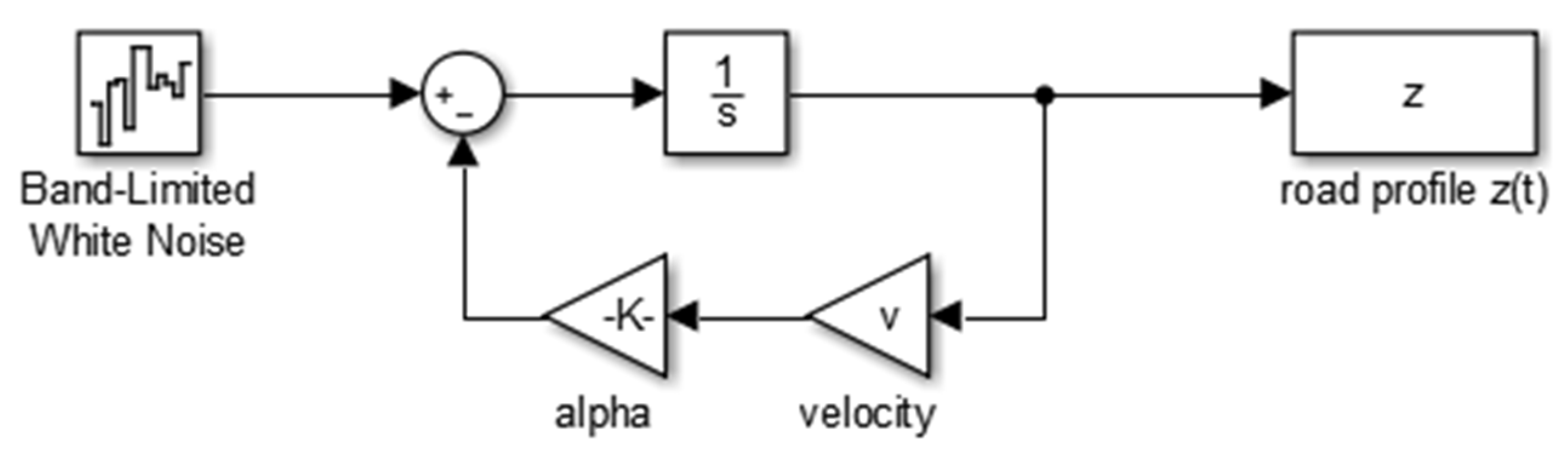
2.1. White Noise Filtration

A white noise signal can be transformed to the road profile either in the spatial or time domain through a first-order linear shape filter. More detailed explanations about the fundamentals and properties of this method can be found in [22,23,24,25]. The simulation using the white noise filtration method uses two models: Without and with a low frequency cut off, as described in [24]. We used a model with a low frequency cut off, where to avoid an increment on the standard deviation during the integration period, the road roughness PSD equation used in ISO 8608 was modified as in [14,15,17,21]:

$$G_{\mathrm{d}}\left(\omega \right)=\frac{2\alpha v{\sigma }^2}{\pi }\frac{1}{{\left(\alpha v\right)}^2+{\omega }^2} \mathrm{or} G_{\mathrm{d}}(\Omega )=\frac{2\alpha {\sigma }^2}{\pi }\frac{1}{{\alpha }^2+{\Omega }^2}$$

(1)

where ${\sigma }^2$ is the road roughness variance, v is a vehicle velocity, ω is an angular frequency in the time domain (rad/s), and Ω is the angular spatial frequency (rad/m). As stated in the literature [14,15,17,22], the parameter α depends on the type of road surface. However, it was shown that α is independent of the road [23,24,25] and it is termed as a low frequency cut off in units of spatial angular frequency (rad/m) [24]. The product αv also means a low frequency cut off but has units of angular temporal frequency (rad/s). If the vehicle runs with a constant velocity v, then the road profile, z(t), with the PSD defined by Equation (1), can be obtained from the output of a linear shape filter expressed by the differential equation:

$$\frac{\mathrm{d}}{\mathrm{d}t}z\left(t\right)=-\alpha vz\left(t\right)+\eta \left(t\right)$$

(2)

where η(t) is a zero-mean Gaussian white noise having a velocity dimension (m/s) with a PSD as $2\alpha v{\sigma }^2$ [14,21]. In our case, the variance was chosen at ${\sigma }^2=4G_{\mathrm{d}}\left({\Omega }_0\right)$ as in most of the literature [23,25,36] with the reference values of PSD at ${\Omega }_0=1 \mathrm{rad}/\mathrm{m}$ given by ISO 8608 [12].

In the spatial domain, the required filter can be expressed as in [24], wherein $z^{\prime }=-\alpha z+\eta \left(x\right)$, where $z^{\prime }=\frac{\partial }{\partial x}z=\frac{1}{v}\frac{\mathrm{d}}{\mathrm{d}t}z\left(t\right)$, η(x) is a zero mean Gaussian white noise having a gradient dimension (m/m) and x is the distance traveled by the vehicle along the road.

2.2. Sinusoidal Approximation

The longitudinal road profile can be mathematically constructed from a set of sinusoidal waves with different wavelengths, amplitudes, and phases in the spatial or time domain. The method in which a sample of Gaussian random signal generated from its spectral description, was proposed by Shinozuka [37,38], has been applied by many authors [10,23,24,25,34,35,39]. In this method, the one-sided PSD spectrum is divided into several frequency bands, and the same number of harmonic samples are generated with the corresponding band frequency and spectral height with random phase angles ${\phi }_i$. Then, the samples are superimposed to generate the road profile in the spatial or time domain by Equations (3) and (4):

$$z\left(x\right)={\displaystyle \sum }_{i=1}^N{Z}_i\cos \left({\Omega }_{i}x+{\phi }_i\right) \mathrm{or} z\left(t\right)={\displaystyle \sum }_{i=1}^N{Z}_i\cos \left({\Omega }_{i}vt+{\phi }_i\right) \mathrm{with}$$

(3)

$$Z_i=\sqrt{2G_{\mathrm{d}}\left({\Omega }_i\right)\Delta \Omega }$$

(4)

where $Z_i$ is the amplitude of i^th harmonic, $N=\left({\Omega }_{\mathrm{U}}-{\Omega }_{\mathrm{L}}\right)/\Delta \Omega$ is the number of frequency bands into which the total PSD spectrum is divided, ${\Omega }_{\mathrm{U}}, {\Omega }_{\mathrm{L}}$ are the upper and lower spatial frequencies in the PSD spectrum (rad/m), $\Delta \Omega$ is the width of each frequency band, ${\Omega }_i={\Omega }_{\mathrm{L}}+\left(i-1\right)\Delta \Omega$ is the spatial frequency of i^th harmonic or i^th frequency band. The phase angle of i^th harmonic ${\phi }_i$ was uniformly distributed in the interval (0, 2π).

2.3. Moving Average of White Noise

The moving average of white noise is a convolution of a kernel Function $g\left(x\right)$ with an infinitesimal “white noise” process having the variance equal to the spatial discretization step dx. For the road profile $z\left(x\right)$ with the standard deviation σ, one denotes by $\tilde{z}\left(x\right)$ a normalized profile, i.e., $\mathrm{E}\left[\tilde{z}\left(x\right)\right]=0$ and $\vee \left[\tilde{z}\left(x\right)\right]=1$. Therefore, for the zero mean profile, $z\left(x\right)=\sigma \tilde{z}\left(x\right)$ with the spectrum $G_{\mathrm{d}}(\Omega )=G_0(\Omega ){\sigma }^2$, where $G_0(\Omega )$ is the spectrum of the normalized road profile $\tilde{z}\left(x\right),$ this approach allows using the same spectrum for all the roads. Consider a kernel function $g\left(x\right)$, which is normalized according to condition ${{\displaystyle \int }}^{ }g{\left(x\right)}^2\mathrm{d}x=1$. Using the kernel $g\left(x\right)$, it can be modelled as stationary and non-stationary Gaussian models, stationary and non-stationary Laplace models, and the hybrid model [31,33].

The standardized Gaussian process can be approximated by:

$$\tilde{z}\left(x\right)\approx {{\displaystyle \sum }}^{ }g\left(x-x_i\right)z_i\sqrt{\mathrm{d}x}$$

(5)

where all the $z_i$ are independent standard Gaussian random variables, while dx is the discretization step. In the case of the symmetric kernel, i.e., $g\left(-x\right)=g\left(x\right)$, the spectrum $G_{\mathrm{d}}(\Omega )$ of $z\left(x\right)$ uniquely defines the kernel $g\left(x\right)$ since:

$$G_{\mathrm{d}}(\Omega )=\frac{1}{2\pi }{\left|ℱg(\Omega )\right|}^2$$

(6)

where $ℱg(\Omega )$ stands for the Fourier transform. For symmetric kernels, their Fourier transform is given by:

$$ℱg(\Omega )=\sqrt{2\pi G_{\mathrm{d}}(\Omega )}$$

(7)

The model represents a non-stationary Gaussian process if we consider the durations and sizes of standard deviations. Assume that the normalized profile $\tilde{z}\left(x\right)$ consists of M equally long blocks $L=L_{\mathrm{p}}/M$, where the variance is constant and equal to $r_j=\frac{{\sigma }_j^2}{{\sigma }^2}, j=1, . . . ,M$, hence:

$$\frac{1}{M}{{\displaystyle \sum }}_{j=1}^M{r}_j=1$$

(8)

Using the moving average of white noise defines a smooth profile $z\left(x\right)$. Let $s_0=0<s_1<···<s_M=L_{\mathrm{p}}$, where $s_j-s_{j-1}=L_{\mathrm{p}}/M$, and define the ${\tilde{z}}_j\left(x\right)$ process for all $0\le x\le L_{\mathrm{p}}$ as follows:

$${\tilde{z}}_j\left(x\right)\approx {\displaystyle \sum }_{s_{j-1}<x_i<s_j}g\left(x-x_i\right)\sqrt{r_j}{z}_i\sqrt{\mathrm{d}x}$$

(9)

Finally, the road profile $z\left(x\right)$ of the non-stationary Gaussian process is given by:

$$z\left(x\right)=\sigma \tilde{z}\left(x\right)=\sigma {\displaystyle \sum }_{j=1}^M{\tilde{z}}_j\left(x\right)$$

(10)

The non-stationary Laplace model is obtained by replacing $r_j$ in Equation (9) by the independent gamma random variables $R_j$ having a probability distribution function:

$$f_R\left(r\right)=\frac{{\theta }^{\theta }}{\mathsf{\Gamma }\left(\theta \right)}{r}^{\theta -1}{e}^{-r\theta }$$

(11)

The gamma distribution has a shape parameter θ and scale ${\theta }^{-1}.$ Traditionally, another parameterization is used in Laplace modelling, viz., $\beta =1/\theta$. If the value of the shape parameter $\beta$ is close to zero, then the Laplace process approaches the Gaussian process. The shape parameter $\beta$ of the Laplace process can also be computed from the kurtosis $\kappa$ of the process z(x), namely $\beta =\left(\kappa -3\right)/3$ [33].

3. Implementation of Simulations

Using all three methods discussed in the previous section, the samples of road profile corresponding to the ISO road class B ($G_{\mathrm{d}}(\Omega )=G_{\mathrm{d}}\left({\Omega }_0\right){\left(\frac{\Omega }{{\Omega }_0}\right)}^{-w}; w=2; {\Omega }_0=1 \mathrm{rad}/\mathrm{m}; G_{\mathrm{d}}\left({\Omega }_0\right)=4\times {10}^{-6} {\mathrm{m}}^3$ [12]) were generated through MATLAB™. There is the suggestion that the lower spatial frequency limit has no reason to measure lower than $n_{\mathrm{L}}=0.01$ cycles/m for on-road vehicles and 0.05 cycles/m for off-road vehicles [12]. For the vibration analysis of suspension on-road vehicles, an upper spatial frequency limit of $n_{\mathrm{U}}=10$ cycles/m has been suggested by considering the low pass filtering effect due to the tire enveloping. For the spatial angular frequency, this means the range of $2\pi \times 0.01\le \Omega \le 2\pi \times 10$ rad/m.

3.1. White Noise Filtration

We implemented a white noise filtration method for the generation of road profile expressed by Equation (2). Using the Simulink model (Figure 1), we solved the equations using the Runge-Kutta method. In the provided model, the “band-limited white noise” block generates white noise with the specified parameters. The ideal white noise is a mathematical convenience and cannot be generated numerically due to its infinite variance, but an approximation in the form of band-limited white noise is useful for simulation. We are taking into account, that the band-limited white noise block specifies a two-sided spectrum, where the parametric units have a dimension as Hz. To get a one-sided averaged PSD, where the units are the square of the magnitude per unit of radial frequency (Mag^2/(rad/sec), we need to multiply the block delivered value by π, i.e., $2\pi \alpha v{\sigma }^2$ instead $2\alpha v{\sigma }^2$. Then, the value of parameter α is equal to 0.127 rad/m [23,25].

To accommodate the lowest frequency harmonic ${\Omega }_{\mathrm{L}}$, the required length of road will be $L\ge \frac{1}{n_{\mathrm{L}}}=100 \mathrm{m}.$ According to the sampling theorem [40], the required step size of x will be $\Delta x\le \frac{1}{2n_{\mathrm{U}}}=0.05 \mathrm{m}$. In this case, the sampling time is equal to $\frac{1}{2n_{\mathrm{U}}v}$ for our model in Simulink. For a smoother profile, a smaller step can be chosen, but it will cause an increase in the required computational efforts.

3.2. Sinusoidal Approximation

For sinusoidal approximation in the time domain, we wrote the MATLAB code. It is noted in the ISO 8608 standard that: “In the literature, a two or more straight-line fitting is often used, but the standardization of a method which guarantees a unique solution is practically impossible”. Accordingly, to get more possibilities to control the road profile, we changed the linear fitting proposed by ISO in Equation (4) to two split fittings offered by Andrén [27]:

$$G_0(\Omega )=\{\begin{array}{ccc}{G}_{\mathrm{d}}\left({\Omega }_0\right){\Omega }^{-w_1}& \mathrm{for}& \Omega \le {\Omega }_1\\ G_{\mathrm{d}}\left({\Omega }_0\right){\Omega }^{-w_2}& \mathrm{for}& {\Omega }_1\le \Omega \le {\Omega }_2\\ G_{\mathrm{d}}\left({\Omega }_0\right){\Omega }^{-w_3}& \mathrm{for}& {\Omega }_2\le \Omega \end{array}$$

(12)

A lower break frequency at ${\Omega }_1=2\pi \times 0.21 \mathrm{rad}/\mathrm{m}$, and the higher break frequency at ${\Omega }_2=2\pi \times 1.22 \mathrm{rad}/\mathrm{m}$ produced the lowest total least square error for the Swedish road network [27]. The frequency band was divided into N = 1000 intervals.

3.3. Moving Average of White Noise

The MATLAB codes presented in [31,33] were adopted and used to simulate the road profiles in the spatial domain by the moving average method with Gaussian and non-stationary Laplace models. The kernel $g\left(x\right)$ was defined by the ISO spectrum, which in the standardized form (variance one, waviness $w=2,$ ${\Omega }_0=1 \mathrm{rad}/\mathrm{m}$) is given by:

$$G_0(\Omega )=\frac{C_0}{{\Omega }^2}, C_0=6.29\times {10}^{-2} {\mathrm{m}}^3, 2\pi \times 0.01\le \Omega \le 2\pi \times 10 \mathrm{rad}/\mathrm{m}$$

(13)

and equal to zero in cases when $\Omega$ lays outside the specified range.

To define the stationary Gaussian model with the ISO spectrum, only one parameter, the roughness coefficient $G_{\mathrm{d}}\left({\Omega }_0\right)$, is required, alternatively to the variance ${\sigma }^2=G_{\mathrm{d}}\left({\Omega }_0\right)/(4C_0)$. To define the non-stationary Laplace model with the ISO spectrum, two parameters are required, the mean roughness $G_{\mathrm{d}}\left({\Omega }_0\right)$, and the Laplace shape parameter $\beta$, which is necessary for modelling the gamma variances. In our case, we chose the single block length $L=100 \mathrm{m}$, $\beta =0.5,$ or kurtosis $\kappa =4.5$. It is essential to note that setting the parameter $\beta$ equal to zero gives the stationary Gaussian case.

To define the non-stationary Gaussian model with the ISO spectrum, we generated r_j as a uniform random number in the range (0.25, 4) and normalized it to match Equation (8). For the moving average of white noise, the discretization step set $\mathrm{d}x=0.05 \mathrm{m}$, is equal to the reciprocal of the sampling frequency. Note that in the code, the same sample of a Gaussian white noise has been used to generate the Gaussian and non-stationary Laplace models of the road profile. The same function kernel g(x) implemented with different parameters allows facilitating a visual comparison of the simulated profiles. Moreover, due to this reason, all random generations take the same seed value, and the time-domain data are converted to the spatial domain. The total length of the profile was chosen as L_p = 1000 m.

4. Simulation Results and Discussion

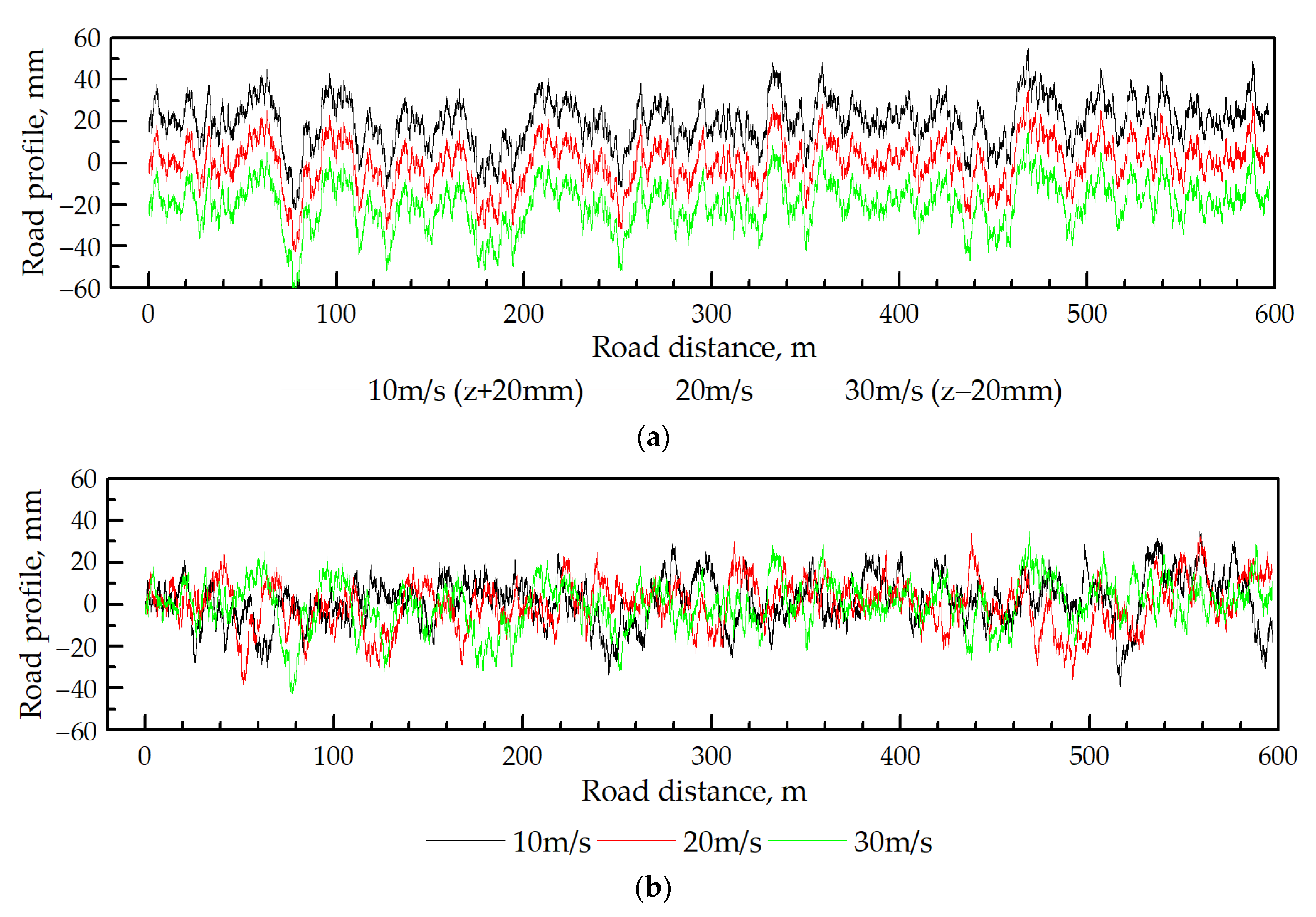
4.1. White Noise Filtration

The simulation of road profile in the time domain using the white noise filtration method for three profile passing velocity values v = 10, 20, and 30 m/s was performed. Initially, calculations have been done choosing sample time values of 0.05/10, 0.05/20, and 0.05/30 s, which are equal to the required minimal time, according to the sampling theorem. The simulation times were set to pass all profile lengths of 1000 m, respectively. Next, calculations were performed using the smallest sample time value. All the obtained results were converted to the spatial domain, as presented in Figure 2. As must be expected, the profiles obtained from the first calculations are identical (Figure 2a). This method is beneficial since it could be used together with other simulations at the same time. However, the appropriate simulation parameters must be used. For example, if the velocity value changes, the sample time value must be changed as well. Otherwise, as seen from Figure 2b, the spatial road profile changes depend on the velocity similar to the roughness peaks that decrease with the velocity and the profiles that shrink when the sample time decreases. The main disadvantage of the implemented method is the lack of full control over the various characteristics.

Another issue of this method is to ensure the Gaussianity of the generated band-limited white noise and road profile peak elevations. It can be ensured by taking a sufficiently large number of samples, and depends on the type of algorithm and seed used for the generation of random numbers [24]. In this case, it was necessary to generate the various sets of road profile data and save one which is closer to the Gaussian distribution.

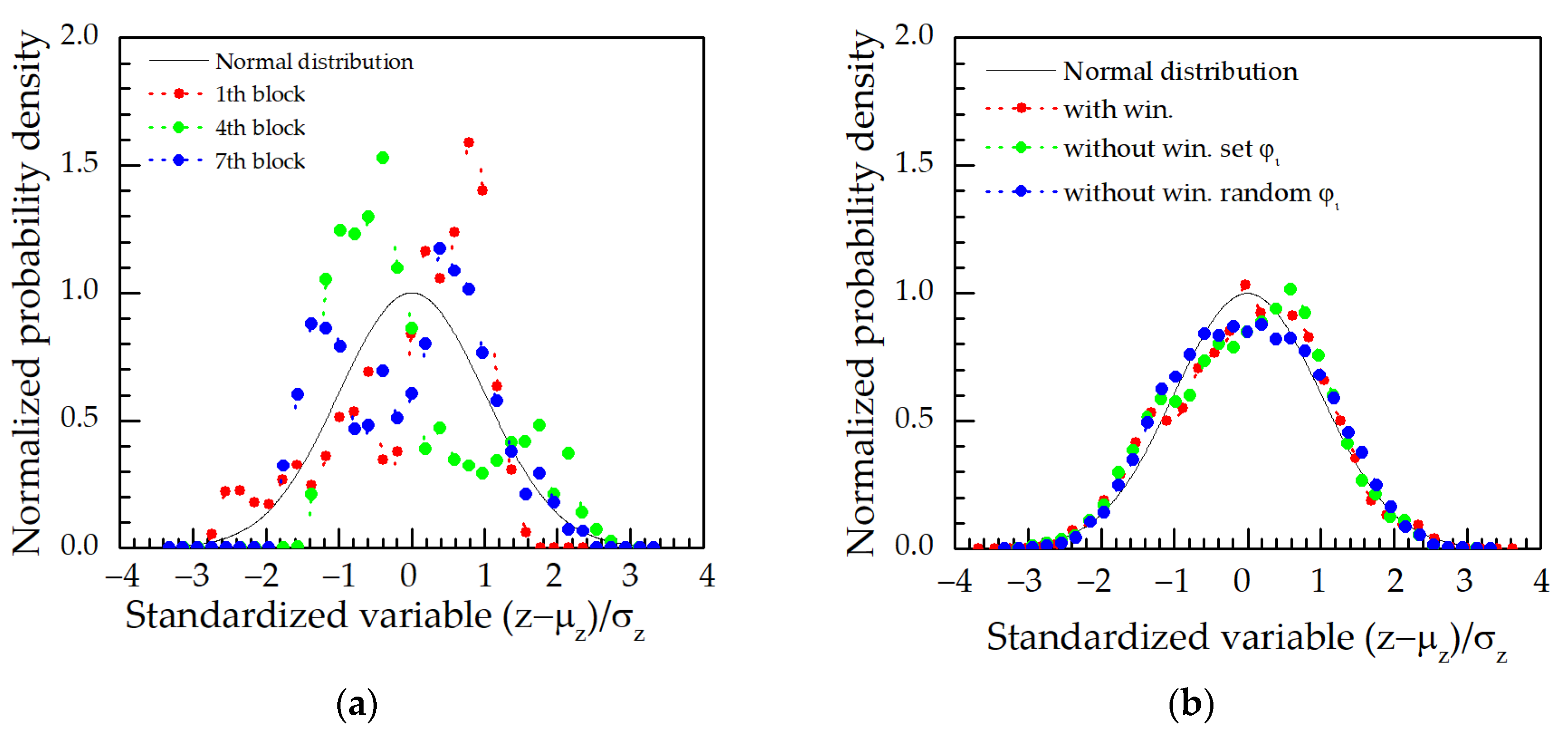
4.2. Sinusoidal Approximation

Simulated road profiles in the spatial domain, using Equations (3) and (4) (sinusoidal approximation) in the range of spatial angular frequency $2\pi \times 0.01\le \Omega \le 2\pi \times 10 \mathrm{rad}/\mathrm{m}$ and equal to zero for values of Ω outside the provided range, are presented in Figure 3a.

As seen in Figure 3a, the road profile cycles at each 100 m distance relates to the lowest frequency value. The mentioned repeatability can be avoided by decreasing the lower limit of Ω value. However, in the extreme case, when the frequency approach is 0, this model outputs an infinite value of the PSD, and thus an infinite variance or elevation, which is outside the realistic values range. The alternative solution to avoid repeatability of profile segments proposes dividing the profile length to blocks and for each block, to generate a new random set of initial phases. Such a technique can develop the appearance of abrupt shift at the connections between the blocks. To minimize this effect, the windowing function was added, in that case, the Welch window with the value of exponent 10 to get a flatter surface:

$$\varpi \left(i\right)=1-{\left(\frac{i-\frac{1}{2}\left(n-1\right)}{\frac{1}{2}\left(n+1\right)}\right)}^{10}$$

(14)

where n is the number of blocks, and i is the number of samples in the block. The result is obtained using the modified algorithm, which removes profile cycling, as shown in Figure 3b. Alternatively, in the case of another approach, it is possible to remove profile segment looping when the different random values of the initial phase φ_i is used as a full road profile (Figure 3c). However, the influence of waves with the long period disappears, and the abrupt shift can appear at any place (Figure 3d).

For a more detailed analysis, the Gaussianity of 100 m blocks having different random initial phases and full profiles without and with windowing was tested (Figure 4). For that purpose, histograms of separate blocks and all profiles were created, the means and standard deviations were calculated and compared with a standard normal distribution. Separate blocks with different sets of random phases have poor Gaussianity. Meanwhile, it becomes better for all profile lengths and even more after windowing (the Kolmogorov-Smirnov test decreases from 0.04 to 0.025). A few reasons could explain the poor Gaussianity: The same set of random initial phases is used in blocks; number N of sinusoids is small and should approach infinity; constant width of frequency band ∆Ω. According to Shinozuka, it is better to use a variable range of sinusoid frequency, depending on the fluctuation of the spectral density [38]. In comparison, the smaller or more delicate spacing gives better corresponding between the generated and target spectrums in the region where the fluctuation of spectral density is more rapid.

The sinusoidal approximation has some advantages and drawbacks. The advantages include the ability to control much more parameters (variance, waviness, number of sinusoids, and its frequency) or investigate the influence of one parameter. In addition, sinusoidal approximation allows obtaining any number of successive differentiations of the road profile height z without going through the numerical differentiation to avoid numerical errors [24]. The main disadvantage of this method is the greater computation time for profile generation. The alternative method is provided by Shinozuka [38,41], Hu, and Schiehlen [42], where they proposed to express Equation (3) in the form of discrete Fourier transform and to obtain the spatial domain road signal through the discrete inverse FFT algorithm. The main advantage of the FFT technique is that this method is much more computationally efficient.

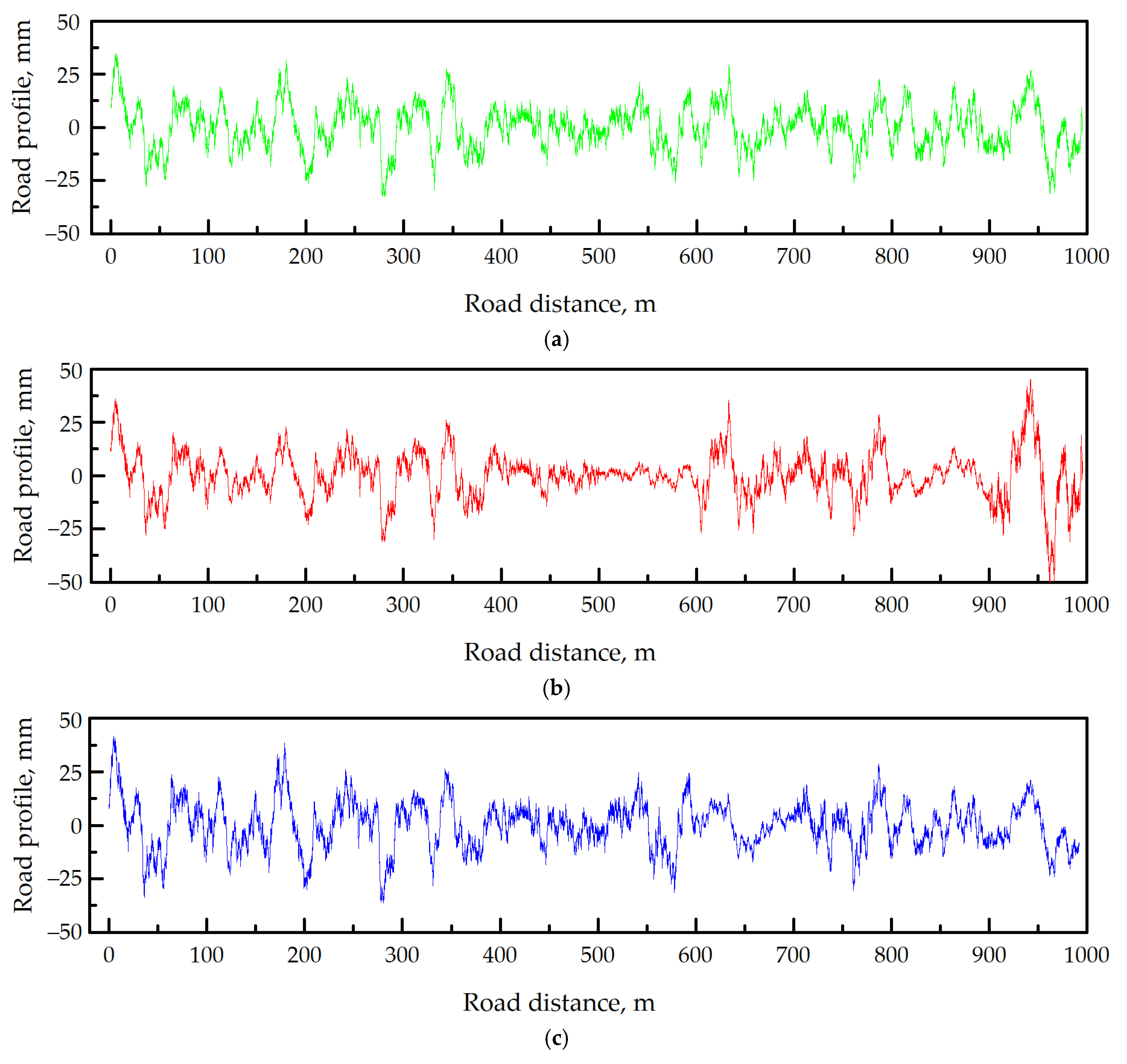
4.3. Moving Average of White Noise

As mentioned in Chapter 2, using the kernel $g\left(x\right)$ the smooth profile $z\left(x\right) \mathrm{can} \mathrm{be} \mathrm{simulated}$, by the various models. Results of the stationary Gaussian, non-stationary Gaussian, and Laplace models are shown in Figure 5a–c. The abrupt shift and looping of the profile is absent in all cases. From the profile z(x) differences (Figure 5d), it is clearly seen that the Gaussian and Laplace’s highest stationarities stay in different blocks. The reason for such a situation is related to another mechanism of random number generation, although it is the same seed value. The evaluated root mean square values of amplitude are 10.4, 11, and 10.8 mm for stationary Gaussian, non-stationary Gaussian, and Laplace models, respectively. For comparison, they are 10.2 and 12.2 mm for sinusoidal approximation and white noise filtration models, respectively.

The observed distributions for stationary and non-stationary Gaussian models show a good correspondence with the standardized normal distribution probability density function. Moreover, the observed distribution for the non-stationary Laplace model is in reasonable compliance with the fitted Laplace probability density function, as shown in Figure 6.

Comparison of the PSD spectra of generated road profiles with the target ISO PSD spectrum is presented in Figure 7. The results of all the methods correspond with the ISO PSD spectrum except the white noise filtration case. Its value is 2.5 ($\sqrt{2\pi }$) times smaller and could be explained due to the different use of a factor of ($1/2\pi )$ either in the expression of Fourier transform or inverse Fourier transform or the use of a factor of ($1/\sqrt{2\pi }$) in both expressions in the band-limited white noise block.

The essential features for all used methods with their own advantages and disadvantages are described in

Table 2. Advantages and disadvantages of road profile creating methods.

Method	Advantages	Disadvantages
White noise filtration	Direct use in Simulink.	Only three parameters: $\mathrm{Low} \mathrm{frequency} \mathrm{cut} \mathrm{off} \mathsf{\alpha }; \mathrm{velocity} v, \mathrm{and} \mathrm{variance} {\sigma }^2=4G_{\mathrm{d}}\left({\Omega }_0\right)$. One must use the appropriate simulation parameters to get correct results (velocity, sample time).
Sinusoidal approximation	Differentiations without going through numerical differentiation. Maximum possible parameters.Possible various PSD approximations.	Repeatability of profile segments or abrupt shift. Greater computation time. Only stationary Gaussian processes.
Moving average of white noise	Possible various PSD approximations. No repeatability of profile segments. Possible stationary or non-stationary Gaussian/Laplace processes.

.

5. Conclusions

The analysis and performed research on artificial road profile generation, according to the standard defined values for each road classification data, reveal the great potential of the method for vehicle suspension, driving dynamics, and car body dynamic response simulations rather than the experimental research. The obtained analysis of road longitudinal profile results allows stating the following conclusions:

The white noise filtration method easily provides a nice and suitable output, as shown in the performed simulations results. This method uses only two variables variation σ² and low-frequency boundary α. The method is simple, but in the case of unadjusted parameter values, the profile floats away and therefore, the roughness amplitude and period draughts away. This method is sensitive to the virtual driving velocity, as well. The positive side in this method is the feature, which is the case when the variation σ² fits the road profile with ω = 2, according to the corresponding ISO standard. This method does not generate an identical profile picture for every 100 m of road profile, as it happens using the method of harmonic functions.

The sinusoidal approximation is the most time-consuming method and generates profile fragments of a certain length. This length depends on the lowest accepted frequency, which in our case is equal to 100 m. The application of randomized harmonic functions creates accidental jumps, which are smoothed using the Welch envelope function with the 10th order of magnitude, allowing us to flatten the profile and analyze the various combinations of frequency patterns.

Implementing the method of moving average avoids profile fragment cloning, and allows various models of profile generation (Gaussian, Laplace) with several values of w in different ranges of frequencies, which cover broader cases than prescribed in the ISO standard.

Finally, all the analyzed methods are useful for road profile generation, but no general method for all the cases of modelling was found. The moving average of the white noise filtration method has a prospective for broader use due to the best compliance to the desired road profile shape and fast computation procedure. Nevertheless, special attention should be paid to the issue of vehicle velocity in the simulation process.

Future implementation of the proposed road synthesis methods, falling into the desired ISO-defined road category, can decrease the time of vehicle dynamic behavior test, add more features into the real object testing program, and provide a chance to create applications directly in the vehicle suspension testbench. The provided methodology allows the inclusion of new requirements for roads, which can appear with future road roughness standard requirements.

References

1. Sayers, M.W.; Karamihas, S.M. The Little Book of Profiling: Basic Information about Measuring and Interpreting Road Profiles; Regent of the University of Michigan: New York, NY, USA, 1998. [Google Scholar]
2. Loprencipe, G.; Cantisani, G. Unified Analysis of Road Pavement Profiles for Evaluation of Surface Characteristics. Mod. Appl. Sci. 2013, 7, 1. [Google Scholar] [CrossRef]
3. Bitelli, G.; Simone, A.; Girardi, F.; Lantieri, C. Laser Scanning on Road Pavements: A New Approach for Characterizing Surface Texture. Sensors 2012, 12, 9110–9128. [Google Scholar] [CrossRef] [PubMed]
4. Martin, D.J.; Nelson, P.M.; Hill, R.C. Measurement and Analysis of Traffic-Induced Vibrations in Buildings; TRRL Supplementary Report 402; Transport and Road Research Laboratoty: Crowthorne, Berkshire, UK, 1978. [Google Scholar]
5. Watts, G.R. The Effects of Traffic Induced Vibrations on Heritage Buildings: Further Case Studies; Research Report 207; Eff. Traffic Induc. Vib. Herit. Build. Furth. Case Stud.; Transport and Road Research Laboratory (TRRL): Crowthorne, Berkshire, UK, 1989. [Google Scholar]
6. Hajek, J.J.; Blaney, C.T.; Hein, D.K. Mitigation of Highway Traffic-Induced Vibration. In Proceedings of the 2006 Annual Conference of the Transportation Association of Canada, Charlottetown, PE, Canada, 17–20 September 2006. [Google Scholar]
7. Sayers, M.W.; Gillespie, T.D.; Queiroz, C.A.V. The international road roughness experiment: A basis for establishing a standard scale for road roughness measurements. Transp. Res. Rec. 1986, 1084, 76–85. [Google Scholar]
8. Paterson, W.D.O. Road Deterioration and Maintenance Effects: Models for Planning and Management; World Bank: Washington, DC, USA, 1987; ISBN 978-0-8018-3590-2. [Google Scholar]
9. Hassan, R.; Mcmanus, K.; Holden, J. Predicting Pavement Deterioration Modes Using Waveband Analysis. Transp. Res. Rec. 1999. [Google Scholar] [CrossRef]
10. Ngwangwa, H.M.; Heyns, P.S.; Labuschagne, F.J.J.; Kululanga, G.K. Reconstruction of road defects and road roughness classification using vehicle responses with artificial neural networks simulation. J. Terramechanics 2010, 47, 97–111. [Google Scholar] [CrossRef] [Green Version]
11. Wambold, J.C. The measurement and data analysis used to evaluate highway roughness. Wear 1979, 57, 117–125. [Google Scholar] [CrossRef]
12. ISO 8608:2016. Available online: https://www.iso.org/cms/render/live/en/sites/isoorg/contents/data/standard/07/12/71202.html (accessed on 11 May 2020).
13. Loprencipe, G.; Zoccali, P. Use of generated artificial road profiles in road roughness evaluation. J. Mod. Transp. 2017, 25, 24–33. [Google Scholar] [CrossRef] [Green Version]
14. Hać, A. Suspension optimization of a 2-DOF vehicle model using a stochastic optimal control technique. J. Sound Vib. 1985, 100, 343–357. [Google Scholar] [CrossRef]
15. Giua, A.; Melas, M.; Seatzu, C.; Usai, G. Design of a Predictive Semiactive Suspension System. Veh. Syst. Dyn. 2004, 41, 277–300. [Google Scholar] [CrossRef]
16. Yoshimura, T. A semi–active suspension of passenger cars using fuzzy reasoning and the field testing. Int. J. Veh. Des. 1998, 19, 150–166. [Google Scholar] [CrossRef]
17. ElMadany, M.M.; El-Tamimi, A. On a subclass of nonlinear passive and semi-active damping for vibration isolation. Comput. Struct. 1990, 36, 921–931. [Google Scholar] [CrossRef]
18. Faris, W.; BenLahcene, Z.; Hasbullah, F. Ride quality of passenger cars: An overview on the research trends. Int J. Veh. Noise Vib. 2012, 8, 185–199. [Google Scholar] [CrossRef]
19. Melcer, J.; Lajčáková, G. Numerical simulation of vehicle motion along the road structure. Rocz. Inż. Bud. 2012, 12, 37–42. [Google Scholar]
20. Bogsjö, K.; Rychlik, I. Vehicle fatigue damage caused by road irregularities. Fatigue Fract. Eng. Mater. Struct. 2009, 32, 391–402. [Google Scholar] [CrossRef]
21. Schiehlen, W. White noise excitation of road vehicle structures. Sadhana 2006, 31, 487–503. [Google Scholar] [CrossRef] [Green Version]
22. Yonglin, Z.; Jiafan, Z. Numerical simulation of stochastic road process using white noise filtration. Mech. Syst. Signal. Process. 2006, 20, 363–372. [Google Scholar] [CrossRef]
23. Tyan, F.; Hong, Y.-F.; Shun, R.; Tu, H.; Jeng, W. Generation of Random Road Profiles. J. Adv. Eng. 2009, 4, 151–156. [Google Scholar]
24. Dharankar, C.S.; Hada, M.K.; Chandel, S. Numerical generation of road profile through spectral description for simulation of vehicle suspension. J. Braz. Soc. Mech. Sci. Eng. 2017, 39, 1957–1967. [Google Scholar] [CrossRef]
25. Goenaga, B.J.; Fuentes Pumarejo, L.G.; Mora Lerma, O.A. Evaluation of the methodologies used to generate random pavement profiles based on the power spectral density: An approach based on the International Roughness Index. Ing. Investig. 2017, 37, 49. [Google Scholar] [CrossRef] [Green Version]
26. Dodds, C.J.; Robson, J.D. The description of road surface roughness. J. Sound Vib. 1973, 31, 175–183. [Google Scholar] [CrossRef]
27. Andren, P. Power spectral density approximations of longitudinal road profiles. Int. J. Veh. Des. 2006, 40, 2–14. [Google Scholar] [CrossRef]
28. Charles, D. Derivation of Environment Descriptions and Test Severities from Measured Road Transportation Data. J. IES 1993, 36, 37–42. [Google Scholar] [CrossRef]
29. Bruscella, B.; Rouillard, V.; Sek, M. Analysis of Road Surface Profiles. J. Transp. Eng. 1999, 125, 55–59. [Google Scholar] [CrossRef]
30. Rouillard, V. Decomposing pavement surface profiles into a Gaussian sequence. Int. J. Veh. Syst. Model. Test. 2009, 4, 288. [Google Scholar] [CrossRef]
31. Bogsjö, K.; Podgórski, K.; Rychlik, I. Models for road surface roughness. Veh. Syst. Dyn. 2012, 50, 725–747. [Google Scholar] [CrossRef]
32. Johannesson, P.; Rychlik, I. Laplace Processes for Describing Road Profiles. Procedia Eng. 2013, 66, 464–473. [Google Scholar] [CrossRef] [Green Version]
33. Johannesson, P.; Rychlik, I. Modelling of road profiles using roughness indicators. Int. J. Veh. Des. 2014, 66, 317. [Google Scholar] [CrossRef]
34. Sun, L. Simulation of pavement roughness and IRI based on power spectral density. Math. Comput. Simul. 2003, 61, 77–88. [Google Scholar] [CrossRef]
35. Agostinacchio, M.; Ciampa, D.; Olita, S. The vibrations induced by surface irregularities in road pavements—A Matlab® approach. Eur. Transp. Res. Rev. 2014, 6, 267–275. [Google Scholar] [CrossRef] [Green Version]
36. Sun, L.; Kennedy, T.W. Spectral Analysis and Parametric Study of Stochastic Pavement Loads. J. Eng. Mech. 2002, 128, 318–327. [Google Scholar] [CrossRef]
37. Shinozuka, M.; Jan, C.-M. Digital simulation of random processes and its applications. J. Sound Vib. 1972, 25, 111–128. [Google Scholar] [CrossRef]
38. Shinozuka, M. Monte Carlo solution of structural dynamics. Comput. Struct. 1972, 2, 855–874. [Google Scholar] [CrossRef]
39. Gorges, C.; Öztürk, K.; Liebich, R. Road classification for two-wheeled vehicles. Veh. Syst. Dyn. 2018, 56, 1289–1314. [Google Scholar] [CrossRef]
40. Shannon, C.E. Communication in the Presence of Noise. Proc. IRE 1949, 37, 10–21. [Google Scholar] [CrossRef]
41. Shinozuka, M.; Deodatis, G. Simulation of Stochastic Processes by Spectral Representation. Appl. Mech. Rev. 1991, 44, 191–204. [Google Scholar] [CrossRef]
42. Hu, B.; Schiehlen, W. On the simulation of stochastic processes by spectral representation. Probabilistic Eng. Mech. 1997, 12, 105–113. [Google Scholar] [CrossRef]
Figure 1. Simulink model of first-order linear shape filter according to Equation (2).
Symmetry 13 00068 g001
Figure 2. Simulated road profile using the white noise filtration method for three velocity values v = 10, 20, and 30 m/s: (a) With the required minimal sample time value (spectra are shifted vertically for clarity), (b) with the fixed sample time value 0.05/30 s.
Symmetry 13 00068 g002
Figure 3. Simulated road profiles in the spatial domain using sinusoidal approximation: (a) Without modification, (b) with modification, (c) without windowing and with random φI; and (d) small range of (a,c) cases.
Symmetry 13 00068 g003
Figure 4. Normalized probability density of simulated (a) separate blocks and (b) whole profiles using a method of sinusoidal approximation.
Symmetry 13 00068 g004
Figure 5. Comparison of simulated road profile z(x) using the moving average of white noise: (a) Stationary Gaussian model, (b) non-stationary Gaussian model, (c) non-stationary Laplace model, (d) differences of them.
Symmetry 13 00068 g005aSymmetry 13 00068 g005b
Figure 6. Comparison of non-parametric estimates of probability densities (dashed line with symbol) with (a) standardized normal distribution, (b) fitted Laplace probability density function (solid lines).
Symmetry 13 00068 g006
Figure 7. Power spectral density (PSD) spectra of the ISO 8608 road profile (dashed line) and generated road profiles using: 1—White noise filtration, 2—sinusoidal approximation and moving average of white noise, 3—stationary Gaussian model, 4—non-stationary Gaussian model, 5—non-stationary Laplace model.
Symmetry 13 00068 g007