Deep Neural Network Compression for Plant Disease Recognition

Abstract

Deep neural networks (DNNs) have become the de facto standard for image recognition tasks, and their applications with respect to plant diseases have also obtained remarkable results. However, the large number of parameters and high computational complexities of these network models make them difficult to deploy on farms in remote areas. In this paper, focusing on the problems of resource constraints and plant diseases, we propose a DNN-based compression method. In order to reduce computational burden, this method uses lightweight fully connected layers to accelerate reasoning, pruning to remove redundant parameters and reduce multiply–accumulate operations, knowledge distillation instead of retraining to restore the lost accuracy, and then quantization to compress the size of the model further. After compressing the mainstream VGGNet and AlexNet models, the compressed versions are applied to the Plant Village dataset of plant disease images, and a performance comparison of the models before and after compression is obtained to verify the proposed method. The results show that the model can be compressed to 0.04 Mb with an accuracy of 97.09%. This experiment also proves the effectiveness of knowledge distillation during the pruning process, and compressed models are more efficient than prevalent lightweight models.

1. Introduction

With the development of computational systems in recent years, especially the rapid progress of graphics processing units (GPUs) [1], deep learning (DL) models [2] have made remarkable achievements in many fields, e.g., natural language processing [3], machine translation [4], medical image analysis [5], and many others. Convolutional neural networks (CNNs), as the basic tools of DL, have been widely applied because of their ability to automatically extract features and process high-dimensional images better than other approaches [6,7,8]. In addition, the same is true for the application of CNNs in agriculture; they can always achieve outstanding results, whether in fruit counting [9,10], plant phenotyping [11], or other applications as discussed in the surveys [12,13]. Plant disease identification [14] is also a hot topic in the agriculture-based DL since it directly affects the yields of crops and indirectly relates to human economic benefits. However, it is of high complexity to determine whether plant leaves are diseased by optical observation, and even domain experts cannot identify certain diseases with high accuracy, which also requires considerable manpower and time. The great successes of CNNs in image recognition [15]. Also make the identification of plant leaf diseases with these networks preferable and have led to significant breakthroughs.

Regarding the development of CNNs, neural networks have been developed from the original LeNet [16] to current networks with wider, deeper, and more parameters, such as AlexNet [15] and VGGNet [17]. Although this has yielded greater progress in terms of accuracy, it also brings a large number of parameters, slow reasoning speed, and large memory footprints. Moreover, these problems are amplified in agriculture. Since farms are usually located in resource-constrained areas, the deployment of these models on remote devices would be limited by network bandwidth and delays. On the edge devices, such as mobile devices and Internet of Things devices, due to the characteristics of these resource-constrained devices [18], such massive neural networks cannot be effectively operated. Therefore, it is particularly critical to compress neural networks simply and efficiently.

In the agricultural field, there are few works that focus on the sizes, processing speeds, and resource constraints of neural network models, which are exactly the issues that should be considered. Researchers in [19] deployed a lightweight neural network after knowledge distillation on an agricultural robot platform to distinguish between weeds and crops. In [20,21,22,23], authors used lightweight CNNs to identify diseased crop leaves for easier deployment on embedded devices. However, in a related study of model compression [24], a lightweight network was only one part of the solution. Therefore, a simpler, faster, and more efficient neural network can be obtained by combining other related methods while incurring almost no accuracy loss. In this study, pruning, knowledge distillation, and quantization, which are universally applicable methods, are combined to obtain lower computational burdens and fewer parameters by compressing the lightweight VGGNet and AlexNet, which are then applied to the leaf disease images in the Plant Village dataset [25,26].

The rest of this article is organized as follows: Section 2 briefly describes the latest model compression techniques. Section 3 presents the proposed method and process in detail. Then, the experimental dataset and its settings are introduced, and the results of the proposed method are shown in Section 4. Finally, the work of this study is summarized, and thoughts are put forward regarding future work, which may be helpful for other researchers performing related work, in Section 5.

2. Related Works

In the field of DL, the pursuit of model accuracy is an important aspect, but the main challenges of deep neural networks (DNNs) also include determining how to reduce the number of model parameters (the size of the model) and the computational cost. Model compression is a software method, and the application cost is low. Compression does not conflict with hardware acceleration, and the two processes can complement each other, so the resulting models can be better deployed on cloud servers or embedded devices. Researchers in [27,28] confirmed that most of the parameters in a given network model are redundant, and it is very possible to establish a “simple” network by removing redundant parameters without affecting the accuracy. The obtained neural network model has lower complexity and can be deployed and applied more conveniently.

2.1. Pruning

2.1.1. Pruning Granularity

As the main method of model compression, pruning can be classified into fine-grained and coarse-grained pruning according to the pruning granularity.

Fine-grained pruning, i.e., unstructured pruning, where the pruning granularity is a single neuron, can remove unimportant neurons according to different criteria. In [27,29], Hessian matrices were proposed for the loss function relative to the weights to remove unimportant connections. However, due to the complexity of the calculation, this also brought additional computational costs. In [30], the weights were set to 0 when they were below a certain threshold, and dense matrices were transformed into sparse matrices to accelerate the calculation. However, it is difficult to achieve substantive acceleration without hardware support and specialized software libraries [31]. Therefore, most of the existing pruning studies have focused on structured pruning, which can also achieve an unstructured compression ratio and acceleration in some cases.

Coarse-grained pruning, i.e., structured pruning, removes an entire structure, and it can accelerate and compress models without special hardware. Among the aspects of structured pruning, since multiply–accumulate (MAC) operations are mostly concentrated in filters, pruning at the filter level is an important consideration. The removal of insignificant filters can reduce the memory requirements and computational budgets of the model. Filter-level pruning can be expressed as an optimization problem:

$$\begin{array}{l}\underset{{\delta }_{ij}}{\min }{\displaystyle \sum _{i=1}^K}{\displaystyle \sum _{j=1}^{n_i}}{\delta }_{ij}ℒ\left(w_j^i\right),\\ \mathrm{s}.\mathrm{t}.{\displaystyle \sum _{j=1}^{n_i}}{\delta }_{ij}=n_{i2},\end{array}$$

(1)

where $w_j^i$ represents the $j$th filter in the $i$th convolution layer, and ${\delta }_{ij}$ is an indicator. When $w_j^i$ is grouped in the removed filter set, its value is 1, and when it is in the reserved filter set, its value is 0. $ℒ(·)$ is used to estimate the importance of the filters. Minimizing Equation (1) is equivalent to removing the least important filters in $n_{i2}$. Therefore, determining how to measure the importance of filters, that is, how to design $ℒ(·)$ becomes a top priority.

In [32], the authors sorted the filters of each convolution layer according to the L1-norm and considered that the smaller the L1-norm of a given layer was, the lower its importance was, which meant that it should be removed. The authors in [33] proposed ThiNet, and the statistical information of the next layer of feature maps was applied to the pruning of the current convolution layer. The authors in [34] proposed applying L1 regularization to the scaling factors of batch normalization (BN) layers to remove filters with lower scaling factors. In [35], the authors considered that the ranks of the feature maps generated by convolution layers determined the amount of information contained, i.e., whether the filters were important, and obtained state-of-the-art results.

2.1.2. Pruning Strategies

Pruning strategies can be classified as one-shot and iterative pruning.

One-shot pruning involves achieving the preset sparsity with just one step and then retraining the model. The process is shown in Figure 1.

Although this strategy is very simple and does not bring additional hyperparameters, it can easily cause accuracy losses that cannot be repaired. In contrast, iterative pruning prunes only a portion of the filters each iteration and retrains the model several times; then, pruning and retraining cycles are repeated to achieve the target sparsity. The authors compared the accuracy of the models obtained after iterative pruning and one-shot pruning in [32], and the results showed that iterative pruning is more effective in compensating for the loss incurred after removing the filter. Researchers in [36] proposed the use of step sparsity to determine the number of filters to be removed in each iteration of pruning.

2.2. Knowledge Distillation

Knowledge distillation, also known as teacher–student training, was proposed in [37]. An experiment demonstrated that a well-trained network uses its output soft labels to guide a simple, small student network through training, and dark knowledge can be easily transferred to the student network without changing its structure. In [38], authors proposed an ensemble of teacher networks to improve the generalization ability of a student network. In [39], the authors used the attention maps of the middle layers of a teacher network to guide the training of the student network, aiming at enabling the student network to learn the feature maps of the teacher more effectively. Researchers in [40] found that if the given teacher and student networks are similar in structure, the student network more easily learns the knowledge of the teacher network, thus saving time when training a complex model.

2.3. Quantization

One method of quantization is to cluster the model weights, which are classified into the same category and can share weight values, to realize the compression of the model; this approach is called vector quantization. In [41], the authors used K-means clustering to implement vector quantization, as this method can achieve a 16–24 time compression ratio, and the accuracy loss lies in an acceptable range. However, the storage of the shared weight codebook and its computation also requires additional resources.

Another method of quantization is to approximate the weights of 32-bit floating-point numbers with fewer bits (such as 16-bit or 8-bit weights), which is called fixed-point quantization. Due to the reduction in the representation bits of weights, the size of the network model can be reduced. Researchers in [42] showed that the use of uint-8 representations to represent the original bits could achieve effective acceleration without sacrificing accuracy. The use of one-bit data to replace the original weight bits is called the binary neural network [43]; although such a network can greatly reduce the network computing and storage costs, determining how to maintain the accuracy after quantization becomes a great challenge.

The application of quantization in the inference stage can accelerate forward propagation and further improve the compression rate and can be combined with other compression methods. For example, in [44], the authors proposed a compression method combining pruning, quantization, and Huffman encoding, and the model could be compressed up to 49 times.

2.4. Lightweight Networks

Unlike pruning and quantization, lightweight networks directly design an efficient model to solve the given problem.

MobileNet [45] decomposes the standard convolution operation into depthwise convolution and pointwise convolution. Depthwise convolution is a convolution operation performed in each independent channel, and pointwise convolution is a 1 $\times$ 1 convolution operation, both of which can greatly reduce the number of required calculations without affecting model accuracy. SqueezeNet [46] achieves approximately equal accuracy to that of AlexNet on ImageNet; moreover, the number of parameters is 50 times less than that of AlexNet.

2.5. DL Architectures for Plant Disease Detection

Using new or modified DL architectures has become a mainstream method for plant disease detection. In [47], the authors proposed a lightweight model and strengthened the generalization performance of the model on a plant disease dataset by transfer learning, which can achieve 89.70% accuracy. In [48,49,50], authors used different DL architectures (such as AlexNet, VGGNet, GoogleNet, and ResNet) to detect plant disease, and achieved promising results, which also promoted the application of DL in agriculture. In [51], the authors introduced a novel DL architecture considering the spot attention mechanism of apple leaf disease and proved its performance is better than traditional DL models.

In this paper, unlike the traditional research that only uses lightweight models [20,21,22,23,47], we combine pruning, distillation, and quantization methods to minimize the size of the model while ensuring accuracy. Compared with existing lightweight models, our proposed model compression method on VGGNet and AlexNet yields more competitive results (see Section 4.3 for details).

3. Methodology

This paper proposes a model compression method for plant disease identification, which includes lightweight, iterative pruning, knowledge distillation, and quantization. The specific flowchart is shown in Figure 2.

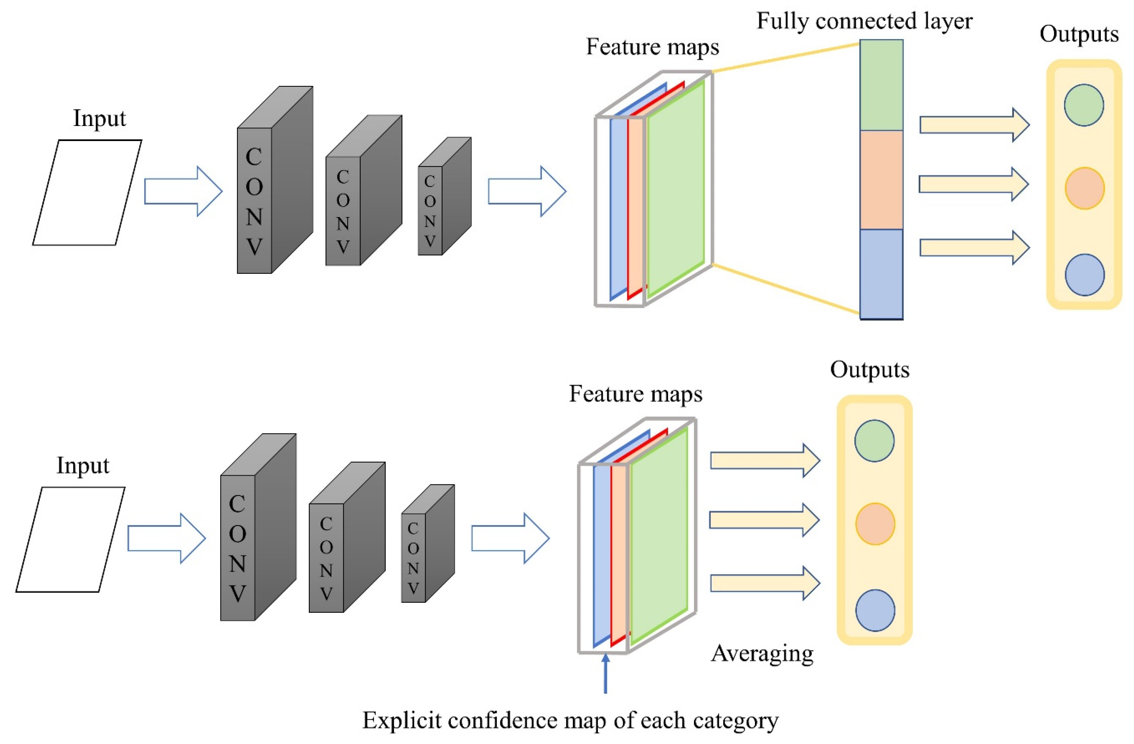
3.1. Lightweight on Fully Connected Layers

Before using correlation compression methods, the weight of the network model should be reduced first. In CNNs, the fully connected layers incur a large number of parameters. As shown in Figure 3, the fully connected layers of VGGNet and AlexNet account for 89.36% and 95.96% of the total number of parameters, respectively. Therefore, to simplify the models, it is necessary to compress the fully connected layers. However, pruning the fully connected layers results in weight sparsity. If there is no special hardware or corresponding software libraries, the acceleration effect is inconspicuous. To solve this problem, in this study, global average pooling (GAP) [52] is used to reduce the burden of the model, as shown in Figure 4. The feature maps of the last convolution layer are pooled to obtain the results so that the extracted features and classification output are directly related. On the one hand, reducing the large number of parameters can reduce the computational cost; on the other hand, it can prevent overfitting, and there is little effect on accuracy.

3.2. Iterative Pruning with Knowledge Distillation

In this study, filter-level structured pruning is applied, where the standard for measuring the importance of the filters is the ranks of the model feature maps [35]; additionally, knowledge distillation is used instead of retraining. The core flow of the proposed algorithm is shown in Algorithm 1.

3.2.1. Iterative Pruning

During the process of pruning, a small batch of input images is used to accurately predict the expected rank of the examined feature map, and Equation (1) can be more specifically expressed as:

$$\begin{gathered} \underset{{\delta }_{ij}}{\min }{\displaystyle \sum _{i=1}^K}{\displaystyle \sum _{j=1}^{n_i}}{\delta }_{ij}ℒ\left(w_j^i\right){\displaystyle \sum _{K=1}^G}\mathrm{Rank}\left(o_j^i(K,:,:)\right), \\ \mathrm{s}.\mathrm{t}.\sum _{j=1}^{n_i}{\delta }_{ij}=n_{i2}, \end{gathered}$$

(2)

where $o_j^i(K,:,:)$ is the matrix of the feature map of input image $K$ generated by $w_j^i$. $\mathrm{Rank}(\cdot )$ is the rank of the feature map matrix that evaluates the average rank across $G$ images.

To distinguish from one-shot pruning, a certain number of filters are removed at each step during iterative pruning. Therefore, in this experiment, a polynomial function Equation (3) is proposed to obtain the step pruning rate.

$$S_t=1-{\left(1-S_f\right)}^{\frac{t+2}{t_f+2}}$$

(3)

where $S_t$ and $S_f$ are the current and target pruning rates, respectively. $t$ is the current pruning step, and $t_f$ is the total number of training steps. In this way, one-shot pruning is avoided, and the pruning of the filters can be completed within the limited number of training steps, which realizes a tradeoff between training time and accuracy.

Algorithm 1. Framework of iterative pruning with knowledge distillation

$∕\ast$Initialization$\ast ∕$

1: Convolution layer index to prune: $L$;

2: Student model pruning rate at step $t$: $S_t\%$;

3: Student model final pruning rate at step $t_f$: $S_f\%$;

$∕\ast$Pretraining$\ast ∕$

4: Training lightweight model $T$;

5: Pretrained student model $S$: $S\leftarrow T$;

$∕\ast$Iterative pruning$\ast ∕$

6: $S_t=1-{\left(1-S_f\right)}^{\frac{t+2}{t_f+2}}$

7: Pruning ($S_t$ $-$ $S_{t-1}$)$\%$ filters of $L$ with feature map ranks;

$∕\ast$Knowledge distillation$\ast ∕$

8: Retraining model $S$ with knowledge distillation with $T$;

9: If ($S_t<S_f$) then Goto Iterative pruning

$∕\ast$Final model$\ast ∕$

10: Return student model $S$;

3.2.2. Retraining

In the traditional three-stage iterative pruning process, after each pruning step, the model is retrained to restore the accuracy loss incurred by pruning. In this paper, knowledge distillation [37] is used instead of retraining to obtain a better precision recovery effect, as shown in Figure 5.

In knowledge distillation, the teacher model uses output soft labels to enable the student model to learn dark knowledge; this process can be defined as:

$$L_{kd}=2T^2\times L_{KL}\left(S_{Stu},S_{Tea}\right)$$

(4)

where the temperature parameter $T$ is used to control the smoothness of the output to preferably transfer the knowledge of the teacher network. $L_{KL}$ is the Kullback–Liebler (KL) divergence between the soft labels of the two network models. The soft label output $S_{stu}$ of the student network can be given by:

$$S_{Stu}=\frac{\exp (z_{\mathrm{s}}/T)}{{\displaystyle \sum _{i=1}^n}\exp (z_{\mathrm{S}}^{\left(i\right)}/T)}$$

(5)

where $z_{\mathrm{S}}$ is the output of the student network without a softmax layer. Equation (5) controls the degree of smoothness of the output, and it is the softmax function when $T=1$. $S_{Tea}$ can also be calculated in this way.

Under the effect of knowledge distillation, the total loss function of the student network model becomes:

$$L_{\mathrm{student}}=\mathsf{\alpha }{L}_{kd}+\mathsf{\beta }\mathrm{CrossEntropy}(z_{\mathrm{S}}, y_{Ture})$$

(6)

where $y_{True}$ denotes the ground-truth label of the output, and the latter term is the classic cross-entropy loss. $\mathsf{\alpha }$ and $\mathsf{\beta }$ are weight hyperparameters.

3.3. Fixed-Point Quantization

Quantization is applied after training, and uint-8 bit-based fixed-point quantization without data calibration is used to compress the matrix of weights.

4. Experimental Evaluation

4.1. Experimental Settings

4.1.1. Datasets

This paper used 54,306 images of diseased and healthy plants under controlled conditions from a public database [25,26], which were obtained by researchers using a standard digital camera with automatic mode. This database includes 38 different classes, each of which contains disease or health data corresponding to a certain plant.

Table 1. Related information about the database images.

Class	Plant Common Name	Plant Scientific Name	Disease Common Name	Disease Scientific Name	Images (Number)
C_1	Apple	Malus domestica	–	–	1645
C_2	Apple	Malus domestica	Apple scab	Venturia inaequalis	630
C_3	Apple	Malus domestica	Black rot	Botryosphaeria obtusa	621
C_4	Apple	Malus domestica	Cedar apple rust	Gymnosporangium juniperi-virginianae	275
C_5	Blueberry	Vaccinium spp.	–	–	1502
C_6	Cherry (and sour)	Prunus spp.	–	–	854
C_7	Cherry (and sour)	Prunus spp.	Powdery mildew	Podosphaera spp.	1052
C_8	Corn (maize)	Zea mays	–	–	1162
C_9	Corn (maize)	Zea mays	Cercospora leaf spot	Cercospora zeae-maydis	513
C_10	Corn (maize)	Zea mays	Common rust	Puccinia sorghi	1192
C_11	Corn (maize)	Zea mays	Northern leaf blight	Exserohilum turcicum	987
C_12	Grape	Vitis vinifera	–	–	423
C_13	Grape	Vitis vinifera	Black rot	Guignardia bidwellii	1180
C_14	Grape	Vitis vinifera	Esca (Black measles)	Phaeomoniella chlamydospora	1383
C_15	Grape	Vitis vinifera	Leaf blight	Pseudocercospora vitis	1076
C_16	Orange	Citrus sinensis	Huanglongbing	Candidatus Liberibacter	5507
C_17	Peach	Prunus persica	–	–	360
C_18	Peach	Prunus persica	Bacterial spot	Xanthomonas campestris	2297
C_19	Pepper, bell	Capsicum annuum	–	–	1477
C_20	Pepper, bell	Capsicum annuum	Bacterial spot	Xanthomonas campestris	997
C_21	Potato	Solanum tuberosum	–	–	152
C_22	Potato	Solanum tuberosum	Early blight	Alternaria solani	1000
C_23	Potato	Solanum tuberosum	Late blight	Phytophthora infestans	1000
C_24	Raspberry	Rubus spp.	–	–	371
C_25	Soybean	Glycine max	–	–	5090
C_26	Squash	Cucurbita spp.	Powdery mildew	Erysiphe cichoracearum, Sphaerotheca fuliginea	1835
C_27	Strawberry	Fragaria spp.	–	–	456
C_28	Strawberry	Fragaria spp.	Leaf scorch	Diplocarpon earlianum	1109
C_29	Tomato	Lycopersicum esculentum	–	–	1591
C_30	Tomato	Lycopersicum esculentum	Bacterial spot	Xanthomonas campestris pv. Vesicatoria	2127
C_31	Tomato	Lycopersicum esculentum	Early blight	Alternaria solani	1000
C_32	Tomato	Lycopersicum esculentum	Late blight	Phytophthora infestans	1909
C_33	Tomato	Lycopersicum esculentum	Leaf mold	Fulvia fulva	952
C_34	Tomato	Lycopersicum esculentum	Septoria leaf spot	Septoria lycopersici	1771
C_35	Tomato	Lycopersicum esculentum	Spider mites	Tetranychus urticae	1676
C_36	Tomato	Lycopersicum esculentum	Target spot	Corynespora cassiicola	1404
C_37	Tomato	Lycopersicum esculentum	Tomato mosaic virus	Tomato mosaic virus (ToMV)	373
C_38	Tomato	Lycopersicum esculentum	ΤYLCV	Begomovirus (Fam. Geminiviridae)	5357
TOTAL:					54,306

lists the information of these 38 classes, including 14 plants and 26 diseases (some plants have only healthy images). Eighty percent of the images were randomly selected as the training set, while the remaining 20% were selected as the test set.

In order to reduce overfitting and improve the generalization ability of the model, rotation mirror and mirror symmetry were used for the training set, as shown in Figure 6. Eighty percent of the images were randomly selected as the training set, while the remaining 20% were selected as the test set.

4.1.2. Configurations

In this experiment, the popular AlexNet and VGGNet-16 models with BN layers were selected for lightweight, pruning, distillation, and quantization and applied to the public database of plant diseases.

During the training process, the initial learning rate is 0.01, and the learning rate drops by 50% every 20 epochs. The stochastic gradient descent with weight-decay = 5 × 10⁻⁴ and momentum = 0.9 is selected as the optimizer. The total number of epochs used to train the original model is 60, and the batch size is set to 32.

For Equation (2), $G$ = 640 (i.e., 20 batches) pictures are used to estimate the average rank of the feature map generated by each filter. Then, during the iterative pruning process of Equation (3), the final pruning rate $S_f$ is set to 0.85, 0.9, and 0.95, and $t_f$ is set to 100. When $t$ = 0, pruning begins, and when $t$ = 100, the final pruning rate is obtained. After pruning all convolution layers, training is continued for 40 additional epochs to restore accuracy, and the learning rate is also decreased by 50% when training is half complete. The detailed process of sparsity-level variation across the training steps during pruning is shown in Figure 7. To prevent the introduction of excessive hyperparameters, the final pruning rate of each layer is the same, and due to the introduction of GAP, pruning does not operate on the last convolution layer. In addition, during knowledge distillation, for Equations (4) and (6), $T$ = 10, $\mathsf{\alpha }$ = 0.1, and $\mathsf{\beta }$ = 0.9. All the experiments were carried out on PyTorch 1.6, CUDA 10.1, and CUDNN 7.6.5 with an NVIDIA GeForce GTX 1080Ti GPU and an Intel i5 10,600 k CPU.

4.2. Experimental Results

In this paper, the numbers of parameters and floating-point operations (FLOPs) are used as the criteria for measuring the model size and computing requirements, which represent the memory occupation and the number of additions and multiplications required for forward propagation; these are common criteria in most related studies. Since the size of each input image is closely related to the required FLOPs, it is necessary to change 224 $\times$ 224 $\times 3$ to 56 $\times$ 56 $\times 3$. As shown in

Table 2. The changes in the accuracy and FLOPs of VGGNet after changing the sizes of the input pictures.

VGGNet	Input Size
	$224\times 224\times 3$	$112\times 112\times 3$	$56\times 56\times 3$
FLOPS	15.53 G	3.97 G	1.06 G
Accuracy	99.59%	99.45%	99.43%
	(+0.0%)	(−0.14%)	(−0.16%)

, within the acceptable range of accuracy decline, the model is accelerated by approximately 15 times.

Table 3. Comparison between the accuracy and parameters of VGGNet and AlexNet with and without GAP.

Model	VGGNet	VGGNet (GAP)	AlexNet	AlexNet (GAP)
Size	512.79 Mb	47.83 Mb	218.06 Mb	7.51 Mb
Accuracy	99.43%	99.37%	99.18%	98.15%
	(+0.0%)	(−0.06%)	(+0.0%)	(−0.03%)

provides various pieces of information about two DL models with and without GAP. This shows that the decrease in model accuracy is within the acceptable range when using GAP, and the number of parameters is greatly reduced. The accuracies of VGGNet and AlexNet decrease by only 0.06% and 0.03%, respectively, reaching 99.37% and 98.15%.

4.2.1. Filter Pruning

Table 4. Change in the number of parameters, accuracy, and FLOPs of VGGNet and AlexNet under different pruning rates.

Model		Original	85%	90%	95%
			Pruning
VGGNet (GAP)	Size	47.83 Mb	1.18 Mb	0.56 Mb	0.16 Mb
	Accuracy	99.37%	99.05%	98.65%	97.20%
		(+0.0%)	(−0.32%)	(−0.72%)	(−2.17%)
	FLOPs	920,230,062	22,974,968	10,764,786	3,240,726
AlexNet (GAP)	Size	7.51 Mb	0.23 Mb	0.12 Mb	0.04 Mb
	Accuracy	98.15%	94.63%	92.19%	87.32%
		(+0.00%)	(−3.52%)	(−5.96%)	(−10.83%)
	FLOPs	21,628,408	1,085,788	666,896	322,200

presents the accuracies, model sizes, and FLOPs of the two architectures at different pruning rates. In addition, VGGNet has better adaptability than AlexNet. Due to the complicated network architecture of VGGNet, even at a 95% pruning rate, the model accuracy is reduced by 2.17%, and the model can be compressed by a factor of 299 and accelerated by a factor of 284. At a pruning rate of 90%, the accuracy is 98.65%, which is a decrease of 0.72%. While its accuracy is almost unchanged at a pruning rate of 85%, the number of parameters is reduced by a factor of 41, and the model is accelerated by a factor of 40.

When the pruning rates of AlexNet are 85%, 90%, and 95%, its accuracy drops from 98.15% by 3.52%, 5.96%, and 10.83%, respectively, while it is compressed by approximate factors of 25, 63, and 188 and accelerated by factors of 20, 32 and 62. Since AlexNet has only five convolution layers, the shallow network architecture causes the filters to have high sensitivity and limited performance, resulting in obvious accuracy losses at a high pruning rate; however, the model size is only 0.04 Mb.

In this experiment, a lightweight network was used as the teacher model before pruning, and a network was used as the student model to perform pruning to further improve the accuracy.

Table 5. Effect of knowledge distillation on the accuracy of VGGNet and AlexNet under different pruning rates.

Model		Original	85%	90%	95%
			Pruning
VGGNet (GAP)	Accuracy	99.37%	99.05%	98.65%	97.20%
	Knowledge distillation
	Accuracy (KD)	_	99.06%	98.74%	97.26%
			(+0.01%)	(+0.09%)	(+0.06%)
AlexNet (GAP)	Accuracy	98.15%	94.63%	92.19%	87.32%
	Knowledge distillation
	Accuracy (KD)	_	94.82%	92.82%	87.63%
			(+0.19%)	(+0.63%)	(+0.31%)

shows the accuracy comparisons before and after knowledge distillation, which are sufficient to prove the effectiveness of using knowledge distillation. It is also observed that when the pruning rate is 90%, the effect of knowledge distillation is best, and the accuracy can be improved by 0.09% and 0.63% for VGGNet and AlexNet, respectively. When the pruning rate is 95%, the accuracy can be improved by 0.06% and 0.31% for VGGNet and AlexNet, respectively. When the pruning rate is 85%, the accuracy can be increased by only 0.01% and 0.19%.

4.2.2. Quantization

In the final step of the proposed method, uint-8 fixed-point quantization is used to further compress the model after pruning and distillation to obtain a higher compression ratio.

Table 6. Change in the model size and accuracy of VGGNet and AlexNet after quantization.

Model		Original	85%	90%	95%
			Pruning
VGGNet (GAP)	Size	47.83 Mb	1.18 Mb	0.56 Mb	0.16 Mb
	Accuracy	99.37%	99.05%	98.65%	97.20%
		(+0.0%)	(−0.32%)	(−0.72%)	(−2.17%)
	Fixed-point quantization with uint-8 bits.
	Size	_	0.29 Mb	0.14 Mb	0.04 Mb
	Accuracy	_	99.06%	98.75%	97.09%
			(−0.31%)	(−0.62%)	(−2.28%)
AlexNet (GAP)	Size	7.51 Mb	0.23 Mb	0.12 Mb	0.04 Mb
	Accuracy	98.15%	94.63%	92.19%	87.32%
		(+0.00%)	(−3.52%)	(−5.96%)	(−10.83%)
	Fixed-point quantization with uint-8 bits.
	Size	_	0.06 Mb	0.03 Mb	0.01 Mb
	Accuracy	_	94.75%	92.78%	87.51%
			(−3.40%)	(−5.37%)	(−10.64%)

(top) shows that the accuracy of VGGNet is not obviously decreased after quantization and increases by 0.01% at a sparsity level of 90%. When the total parameter size is only 0.04 Mb, which is reduced by a factor of 1196, the accuracy can still reach 97.09%, with a drop of merely 2.28% from the original accuracy rate. Especially at a sparsity level of 85%, the accuracy of the model can still reach 99.06%.

AlexNet also exhibits no significant decrease in accuracy after quantization. In Table 6 (bottom), it can be seen that at a sparsity level of 85%, the model size is reduced by a factor of 125. It can be compressed by a factor of 751 after quantization at a high sparsity level of 95%, and the model size is only 0.01 Mb, but the accuracy is 87.51%, 10.64% lower than the original accuracy rate.

Examining the overall effect of quantization, it can be seen that the accuracy losses of the two kinds of network models after quantization are within the acceptable range, and the model sizes can also be compressed approximately 4 times more. Furthermore, due to the decrease in bits, the MAC operations of the convolution layers become simplified, and the forward propagation speed becomes faster.

4.3. Comparsion with Lightweight Model

In order to verify the effectiveness of the proposed method on VGGNet and AlexNet models, we compare compressed versions with the prevalent lightweight model on the same dataset.

Table 7. Various pieces of information about MobileNetV1 and MobileNetV2 on the plant disease dataset.

Model	MobileNetV1	MobileNetV2
Size	12.38 Mb	8.67 Mb
Accuracy	99.20%	98.85%
FLOPs	150,466,304	23,550,528

provides various pieces of information about MobileNet in the same experimental environment as VGGNet and AlexNet. By comparing it with Table 3, we can observe that lightweight networks obtain better results than uncompressed networks. However, as shown in Figure 8, more competitive results can be obtained when these networks are compressed and knowledge-distilled. The accuracy of VGGNet is 0.21% higher than that of MobileNetV2 at an 85% pruning rate, and the number of parameters is greatly reduced. From the perspective of model size and FLOPs, AlexNet is more efficient after pruning, although its performance decreases obviously.

Compared with traditional research using lightweight models on plant disease datasets, the compression method introduced in this paper can provide a better tradeoff between the size and accuracy of the model. Moreover, we can manually adjust the pruning rate to obtain the model we want, allowing it to be better deployed in resource-constrained areas.

5. Conclusions

In this study, due to the limitations of DNN deployment and the low performance of such networks on resource-constrained devices, the applicability of the resulting models in the field of plant diseases is limited. Therefore, in view of the problems faced by farms in remote areas, the VGGNet and AlexNet models are compressed to reduce the number of required parameters and accelerate reasoning. In the compression method, lightweight fully connected layers, pruning, knowledge distillation, and quantization are combined to obtain efficient models with accuracy losses that fall within an acceptable range. The experimental results also show the effectiveness of using knowledge distillation in iterative pruning. Moreover, the compressed model is more suitable for deployment in resource-constrained areas than the lightweight model.

In the following work, on the one hand, it will also be a key issue to find the optimal pruning number of each convolution layer to achieve a balance between accuracy loss and model size and to achieve the best knowledge distillation effect. On the other hand, extending the dataset as much as possible, compressing the models on field-programmable gate arrays (FPGAs), and deploying them in a real farm environment are additional tasks that need to be carried out.

References

1. Chetlur, S.; Woolley, C.; Vandermersch, P.; Cohen, J.; Tran, J.; Catanzaro, B.; Shelhamer, E. Cudnn: Efficient primitives for deep learning. arXiv 2014, arXiv:1410.0759. Available online: https://arxiv.org/abs/1410.0759 (accessed on 3 May 2021).
2. LeCun, Y.; Bengio, Y.; Hinton, G. Deep learning. Nature 2015, 521, 436–444. [Google Scholar] [CrossRef] [PubMed]
3. Young, T.; Hazarika, D.; Poria, S.; Cambria, E. Recent trends in deep learning based natural language processing. IEEE Comput. Intell. Mag. 2018, 13, 55–75. [Google Scholar] [CrossRef]
4. Vaswani, A.; Shazeer, N.; Parmar, N.; Uszkoreit, J.; Jones, L.; Gomez, A.N.; Kaiser, Ł.; Polosukhin, I. Attention is all you need. In Advances in Neural Information Processing Systems; NIPS: Long Beac, CA, USA, 2017; pp. 5998–6008. [Google Scholar]
5. Litjens, G.; Kooi, T.; Bejnordi, B.E.; Setio, A.A.A.; Ciompi, F.; Ghafoorian, M.; Van Der Laak, J.A.; Van Ginneken, B.; Sánchez, C.I. A survey on deep learning in medical image analysis. Med. Image Anal. 2017, 42, 60–88. [Google Scholar] [CrossRef] [Green Version]
6. Girshick, R. Fast r-cnn. In Proceedings of the IEEE International Conference on Computer Vision, Santiago, Chile, 13–16 December 2015; pp. 1440–1448. [Google Scholar]
7. Noh, H.; Hong, S.; Han, B. Learning deconvolution network for semantic segmentation. In Proceedings of the IEEE International Conference on Computer Vision, Santiago, Chile, 13–16 December 2015; pp. 1520–1528. [Google Scholar]
8. Jia, X.; Gavves, E.; Fernando, B.; Tuytelaars, T. Guiding the long-short term memory model for image caption generation. In Proceedings of the IEEE International Conference on Computer Vision, Santiago, Chile, 13–16 December 2015; pp. 2407–2415. [Google Scholar]
9. Rahnemoonfar, M.; Sheppard, C. Deep count: Fruit counting based on deep simulated learning. Sensors 2017, 17, 905. [Google Scholar] [CrossRef] [PubMed] [Green Version]
10. Kang, H.; Chen, C. Fast implementation of real-time fruit detection in apple orchards using deep learning. Comput. Electron. Agric. 2020, 168, 105108. [Google Scholar] [CrossRef]
11. Xiong, J.; Yu, D.; Liu, S.; Shu, L.; Wang, X.; Liu, Z.J.E. A review of plant phenotypic image recognition technology based on deep learning. Electronics 2021, 10, 81. [Google Scholar] [CrossRef]
12. Kamilaris, A.; Prenafeta-Boldú, F.X. Deep learning in agriculture: A survey. Comput. Electron. Agric. 2018, 147, 70–90. [Google Scholar] [CrossRef] [Green Version]
13. Mortensen, A.K.; Dyrmann, M.; Karstoft, H.; Jørgensen, R.N.; Gislum, R. Semantic segmentation of mixed crops using deep convolutional neural network. In Proceedings of the CIGR-AgEng Conference, Aarhus, Denmark, 26–29 June 2016; pp. 1–6. [Google Scholar]
14. Hasan, R.I.; Yusuf, S.M.; Alzubaidi, L. Review of the state of the art of deep learning for plant diseases: A broad analysis and discussion. Plants 2020, 9, 1302. [Google Scholar] [CrossRef]
15. Krizhevsky, A.; Sutskever, I.; Hinton, G.E. Imagenet classification with deep convolutional neural networks. Commun. ACM 2012, 25, 1097–1105. [Google Scholar] [CrossRef]
16. LeCun, Y.; Bottou, L.; Bengio, Y.; Haffner, P. Gradient-based learning applied to document recognition. Proc. IEEE 1998, 86, 2278–2324. [Google Scholar] [CrossRef] [Green Version]
17. Simonyan, K.; Zisserman, A. Very deep convolutional networks for large-scale image recognition. arXiv 2014, arXiv:1409.1556. Available online: https://arxiv.org/abs/1409.1556 (accessed on 3 May 2021).
18. Zhang, C.; Patras, P.; Haddadi, H. Deep learning in mobile and wireless networking: A survey. IEEE Commun. Surv. Tutorials 2019, 21, 2224–2287. [Google Scholar] [CrossRef] [Green Version]
19. McCool, C.; Perez, T.; Upcroft, B. Mixtures of lightweight deep convolutional neural networks: Applied to agricultural robotics. IEEE Robot. Autom. Lett. 2017, 2, 1344–1351. [Google Scholar] [CrossRef]
20. Gonzalez-Huitron, V.; León-Borges, J.A.; Rodriguez-Mata, A.; Amabilis-Sosa, L.E.; Ramírez-Pereda, B.; Rodriguez, H. Disease detection in tomato leaves via CNN with lightweight architectures implemented in Raspberry Pi 4. Comput. Electron. Agric. 2021, 181, 105951. [Google Scholar] [CrossRef]
21. Chen, J.; Wang, W.; Zhang, D.; Zeb, A.; Nanehkaran, Y.A. Attention embedded lightweight network for maize disease recognition. Plant Pathol. 2021, 70, 630–642. [Google Scholar] [CrossRef]
22. Tang, Z.; Yang, J.; Li, Z.; Qi, F. Grape disease image classification based on lightweight convolution neural networks and channelwise attention. Comput. Electron. Agric. 2020, 178, 105735. [Google Scholar] [CrossRef]
23. Chen, J.; Zhang, D.; Nanehkaran, Y.A. Identifying plant diseases using deep transfer learning and enhanced lightweight network. Multimed. Tools Appl. 2020, 79, 31497–31515. [Google Scholar] [CrossRef]
24. Choudhary, T.; Mishra, V.; Goswami, A.; Sarangapani, J. A comprehensive survey on model compression and acceleration. Artif. Intell. Rev. 2020, 53, 5113–5155. [Google Scholar] [CrossRef]
25. Hughes, D.; Salathé, M. An open access repository of images on plant health to enable the development of mobile disease diagnostics. arXiv 2015, arXiv:1511.08060. Available online: https://arxiv.org/abs/1511.08060 (accessed on 3 May 2021).
26. Mohanty, S.P.; Hughes, D.P.; Salathé, M. Using deep learning for image-based plant disease detection. Front. Plant Sci. 2016, 7, 1419. [Google Scholar] [CrossRef] [Green Version]
27. LeCun, Y.; Denker, J.S.; Solla, S.A. Optimal brain damage. In Advances in Neural Information Processing Systems; NIPS: Morgan Kaufmann, CA, USA, 1990; pp. 598–605. Available online: https://dl.acm.org/doi/10.5555/109230.109298 (accessed on 3 May 2021).
28. Denil, M.; Shakibi, B.; Dinh, L.; Ranzato, M.A.; De Freitas, N. Predicting parameters in deep learning. arXiv 2013, arXiv:1306.0543. Available online: https://arxiv.org/abs/1306.0543 (accessed on 3 May 2021).
29. Hassibi, B.; Stork, D.G. Second Order Derivatives for Network Pruning: Optimal Brain Surgeon. In Advances in Neural Information Processing Systems 5; NIPS: Morgan Kaufmann, CA, USA, 1993; pp. 164–171. [Google Scholar]
30. Han, S.; Pool, J.; Tran, J.; Dally, W.J. Learning both weights and connections for efficient neural networks. arXiv 2015, arXiv:1506.02626. Available online: https://arxiv.org/abs/1506.02626 (accessed on 3 May 2021).
31. Han, S.; Liu, X.; Mao, H.; Pu, J.; Pedram, A.; Horowitz, M.A.; Dally, W.J. EIE: Efficient inference engine on compressed deep neural network. ACM SIGARCH Comput. Archit. News 2016, 44, 243–254. [Google Scholar] [CrossRef]
32. Li, H.; Kadav, A.; Durdanovic, I.; Samet, H.; Graf, H.P. Pruning filters for efficient convnets. arXiv 2016, arXiv:1608.08710. Available online: https://arxiv.org/abs/1608.08710 (accessed on 3 May 2021).
33. Luo, J.-H.; Wu, J.; Lin, W. Thinet: A filter level pruning method for deep neural network compression. In Proceedings of the IEEE International Conference on Computer Vision, Venic, Italy, 27–29 October 2017; pp. 5058–5066. [Google Scholar]
34. Liu, Z.; Li, J.; Shen, Z.; Huang, G.; Yan, S.; Zhang, C. Learning efficient convolutional networks through network slimming. In Proceedings of the IEEE International Conference on Computer Vision, Venic, Italy, 27–29 October 2017; pp. 2736–2744. [Google Scholar]
35. Lin, M.; Ji, R.; Wang, Y.; Zhang, Y.; Zhang, B.; Tian, Y.; Shao, L. Hrank: Filter pruning using high-rank feature map. In Proceedings of the IEEE/CVF Conference on Computer Vision and Pattern Recognition, Seattle, WA, USA, 14–19 June 2020; pp. 1529–1538. [Google Scholar]
36. Zhu, M.; Gupta, S. To prune, or not to prune: Exploring the efficacy of pruning for model compression. arXiv 2017, arXiv:1710.01878. Available online: https://arxiv.org/abs/1710.01878 (accessed on 3 May 2021).
37. Hinton, G.; Vinyals, O.; Dean, J. Distilling the knowledge in a neural network. arXiv 2015, arXiv:1503.02531. Available online: https://arxiv.org/abs/1503.02531 (accessed on 3 May 2021).
38. Fukuda, T.; Suzuki, M.; Kurata, G.; Thomas, S.; Cui, J.; Ramabhadran, B. Efficient Knowledge Distillation from an Ensemble of Teachers. In Proceedings of the Interspeech, Stockholm, Sweden, 20–24 August 2017; pp. 3697–3701. [Google Scholar]
39. Zagoruyko, S.; Komodakis, N. Paying more attention to attention: Improving the performance of convolutional neural networks via attention transfer. arXiv 2016, arXiv:1612.03928. Available online: https://arxiv.org/abs/1612.03928 (accessed on 3 May 2021).
40. Mirzadeh, S.I.; Farajtabar, M.; Li, A.; Levine, N.; Matsukawa, A.; Ghasemzadeh, H. Improved knowledge distillation via teacher assistant. In Proceedings of the AAAI Conference on Artificial Intelligence, New York, NY, USA, 7–12 February 2020; pp. 5191–5198. [Google Scholar]
41. Gong, Y.; Liu, L.; Yang, M.; Bourdev, L. Compressing deep convolutional networks using vector quantization. arXiv 2014, arXiv:1412.6115. Available online: https://arxiv.org/abs/1412.6115 (accessed on 3 May 2021).
42. Vanhoucke, V.; Senior, A.; Mao, M.Z. Improving the Speed of Neural Networks on CPUs. 2011. Available online: https://www.researchgate.net/publication/319770111_Improving_the_speed_of_neural_networks_on_CPUs (accessed on 3 May 2021).
43. Courbariaux, M.; Hubara, I.; Soudry, D.; El-Yaniv, R.; Bengio, Y. Binarized neural networks: Training deep neural networks with weights and activations constrained to +1 or −1. arXiv 2016, arXiv:1602.02830. Available online: https://arxiv.org/abs/1602.02830 (accessed on 3 May 2021).
44. Han, S.; Mao, H.; Dally, W.J. Deep compression: Compressing deep neural networks with pruning, trained quantization and huffman coding. arXiv 2015, arXiv:1510.00149. Available online: https://arxiv.org/abs/1510.00149 (accessed on 3 May 2021).
45. Howard, A.G.; Zhu, M.; Chen, B.; Kalenichenko, D.; Wang, W.; Weyand, T.; Andreetto, M.; Adam, H. Mobilenets: Efficient convolutional neural networks for mobile vision applications. arXiv 2017, arXiv:1704.04861. Available online: https://arxiv.org/abs/1704.04861 (accessed on 3 May 2021).
46. Iandola, F.N.; Han, S.; Moskewicz, M.W.; Ashraf, K.; Dally, W.J.; Keutzer, K. SqueezeNet: AlexNet-level accuracy with 50× fewer parameters and <0.5 MB model size. arXiv 2016, arXiv:1602.07360. Available online: https://arxiv.org/abs/1602.07360 (accessed on 3 May 2021).
47. Ale, L.; Sheta, A.; Li, L.; Wang, Y.; Zhang, N. Deep learning based plant disease detection for smart agriculture. In Proceedings of the 2019 IEEE Globecom Workshops (GC Wkshps), Waikoloa, HI, USA, 9–13 December 2019; pp. 1–6. [Google Scholar]
48. Ferentinos, K.P. Deep learning models for plant disease detection and diagnosis. Comput. Electron. Agric. 2018, 145, 311–318. [Google Scholar] [CrossRef]
49. Delnevo, G.; Girau, R.; Ceccarini, C.; Prandi, C. A Deep Learning and Social IoT approach for Plants Disease Prediction toward a Sustainable Agriculture. IEEE Internet Things J. 2021. Available online: https://ieeexplore.ieee.org/abstract/document/9486935 (accessed on 3 September 2021).
50. Tetila, E.C.; Machado, B.B.; Menezes, G.K.; Oliveira, A.D.S.; Alvarez, M.; Amorim, W.P.; Belete, N.A.D.S.; Da Silva, G.G.; Pistori, H. Automatic recognition of soybean leaf diseases using UAV images and deep convolutional neural networks. IEEE Geosci. Remote. Sens. Lett. 2019, 17, 903–907. [Google Scholar] [CrossRef]
51. Yu, H.-J.; Son, C.-H. Leaf spot attention network for apple leaf disease identification. In Proceedings of the IEEE/CVF Conference on Computer Vision and Pattern Recognition Workshops, Seattle, WA, USA, 14–19 June 2020; pp. 52–53. [Google Scholar]
52. Lin, M.; Chen, Q.; Yan, S. Network in network. arXiv 2013, arXiv:1312.4400. Available online: https://arxiv.org/abs/1312.4400 (accessed on 3 September 2021).
Figure 1. The network model performs pretraining first and then prunes once according to the preset evaluation criteria to achieve the target pruning rate. Finally, the model is fine-tuned to obtain the final model.
Symmetry 13 01769 g001
Figure 2. The flowchart of the proposed compression method.
Symmetry 13 01769 g002
Figure 3. The proportions of parameters in each layer of VGGNet and AlexNet. VGGNet has 13 convolution layers, AlexNet has 5 convolution layers, and the FC refers to all the parameters of the fully connected layers.
Symmetry 13 01769 g003
Figure 4. Replacing fully connected layers with GAP.
Symmetry 13 01769 g004
Figure 5. Using the outputs of the teacher network to guide the outputs of the student network.
Symmetry 13 01769 g005
Figure 6. Examples of rotation mirror and mirror symmetry used for Peach Bacterial Spot image: (a) initial; (b) rotated 90°; (c) rotated 180°; (d) rotated 270°; (e) vertical mirror symmetry; (f) horizontal mirror symmetry.
Symmetry 13 01769 g006aSymmetry 13 01769 g006b
Figure 7. The sparsity changes with the increase in the number of pruning steps. A final sparsity of 0.85 is obtained at step 140. The dotted line represents the pruning step and the corresponding sparsity level.
Symmetry 13 01769 g007
Figure 8. Comparison of MobileNet, VGGNet, and AlexNet accuracy on the plant disease dataset as a function of learned model size (a) and FLOPs (b).
Symmetry 13 01769 g008