Study of Liquid Viscosity Effects on Hydrodynamic Forces on an Oscillating Circular Cylinder Underwater Using OpenFOAM^®

Abstract

By neglecting the viscosity of fluid and rotation in flow, the theory of potential flow cannot accurately predict the hydrodynamic forces on the structures under significant viscous effects. In this study, the effects of liquid viscosity on the hydrodynamic forces on a horizontal circular cylinder underwater with a large-amplitude forced oscillation were investigated. The study used a two-dimensional two-phase flow wave tank model based on the viscous fluid theory using the OpenFOAM^® package. The numerical calculations were carried out under different types of liquid (i.e., liquid with different viscosities). The liquid viscosity effects are visually shown by comparison of the various frequency components of the hydrodynamic forces on the cylinder, and the magnitude and phase relations of the viscous shear forces and the pressure forces. By analyzing the distribution characteristics of the flow fields around the circular cylinder, the viscous-effect mechanisms are revealed. It is found that the discrepancies of the contributions of viscous shear forces, and the discrepancies of the vortex effects on the phase and magnitude of the pressure forces lead to the obvious differences among the results under different liquid viscosities.

1. Introduction

In view of design rationality and production safety, accurate prediction of hydrodynamic force on structure has become an important issue today in the ocean engineering realm. As a typical fluid–structure interaction behavior and also a classic hydrodynamic problem, a horizontal circular cylinder with forced oscillation underwater has attracted extensive attention and research. The circular cylinder is an axial-symmetry structure and the oscillation follows simple harmonic motions with characteristic symmetry of the physical quantities and positions.

To simplify the computation, the related early analytic and numerical studies were carried out on the basis of the traditional potential flow theory. The multipole expansion method (MEM) was used to study the issue of a submerged horizontal cylinder in a large-amplitude and reciprocal oscillating mode by Wu (1993) [1]. In the analytic study, the various frequency components of the hydrodynamic forces on the circular cylinder were derived under a linear free-surface boundary condition and a nonlinear body-surface boundary condition. Rahman and Bhatta (1993) [2] proposed an analytical solution to the velocity potential that governs the linear radiation problem, and solved the added mass and damping coefficients of an oscillating vertical circular cylinder. Over a range of oscillating frequencies, the potential analytical solutions were in good agreement with the experimental data. Tyvand and Miloh (1995a, b) used the time series expansion method for the analytic study on the initial impact motion of a circular cylinder, obtaining the hydrodynamic forces on the cylinder and the amplitudes of the radiation waves [3,4]. In these studies, the free-surface condition was also assumed to be linear.

Some numerical investigations considering the nonlinear free-surface condition have been carried out. With combining the boundary element method (BEM) and the finite element method (FEM), the nonlinear morphological properties of the radiation waves induced by an oscillating circular cylinder underwater were studied by Wu and Eatock Taylor (1995) [5]. Greenhow and Moyo (1997) studied respectively totally and partially submerged horizontal circular cylinders under forced motion in and out of water by using a nonlinear BEM, and found significant differences in the free surface morphology [6]. Subsequently, Liu et al. (1999) analyzed the nonlinear radiation water waves generated by the oscillatory motions of a horizontal circular cylinder underwater with the BEM [7]. Based on an explicit solution method with boundary condition decomposition, the vertical forces on a submerged cylinder body in forced heave movements were numerically investigated by Kent and Choi (2007) [8]. The comparison of the triple-frequency components between the acquired numerical results and the previous linear analytical solutions showed some discrepancies. By using a 2-D (two-dimensional) numerical wave tank (NWT) model built up with the BEM, the interaction of a submerged horizontal cylinder body under oscillatory motion and radiation nonlinear waves was calculated by the studies of Guerber et al. (2010, 2012) [9,10]. It was found that the nonlinear free-surface condition has an effect on the double-frequency forces on the cylinder in the oscillating direction.

Because the potential flow theory cannot predict viscous effect, some viscous numerical investigations of the interaction of fluid and oscillating cylindrical structure were conducted. Guilmineau and Queutey (2002) used a 2-D model and numerically studied the vortex shedding from a circular cylinder with oscillatory motions, and found Morison’s equation simplifies the behavior of wave loading, not accounting for effects, such as vortex shedding [11]. The numerical investigations of confined flow over a transverse oscillating rectangular cylinder were carried out by Yang et al. (2005) [12]. The study found that the vortices shedding is entrained by the cylinder motion, and the wake state is dominated by the interactions between the shedding of vortices and the oscillatory motion of cylinder. Incompressible flows around a circular cylinder under forced oscillation were studied by Wu and Shu (2008) using the local domain-free discretization method. The numerical results are in good agreement with the previous experimental data [13]. Pham et al. (2010) studied laminar flow past a transversely oscillating circular cylinder with a viscous flow numerical model in 2-D space [14], and emphatically studied the drag coefficient, the lift coefficient and the vorticity distribution around the body surface. Based on a second order finite volume numerical model, the study on flow past a transverse forced oscillating circular cylinder near a straight wall was carried out by Peter and De (2017) [15]. The interactions of the wake near the wall and the straight-wall layer was promoted because of the straight-wall presence, and the irregular vortex shedding was inhibited.

Compared with the 2-D studies, the 3-D (three-dimensional) space has scaling effects on the fluid–structure interaction. A 3-D numerical model was built by Mittal (2004), and used to investigate the issue of uniform flow past a rotating circular cylinder [16]. It was found that in the same case, the 2-D flow is stable, but, there are centrifugal instabilities of the flow along the cylinder axis in the 3-D space. The wake of a spinning circular cylinder in a free stream was studied by Rao et al. (2013) using a 3-D numerical model [17]. The complexity of 3-D scenario increases under the higher spin rate of the cylinder. Two new steady flow modes and three new non-steady flow modes are found and identified. Wang et al. (2017) investigated the influences of 3-D scaling on the flow induced by an axial oscillating cylinder with bottom-attached disks, and obtained the hydrodynamic coefficients with a viscous fluid numerical model [18]. Three patterns of vortex shedding are found, and cause the 3-D effects on the flow field around the cylinder. Jacono et al. (2018) numerically studied the wake of a rotating cylinder under forced linearly transverse oscillating in a free stream, and focused on the transition to 3-D flow in the wake [19]. The results showed that the change of the linear mode leads to the non-monotonic complex relationships among the response frequency, the response amplitude and the reduced velocity, then causes the transition to 3-D flow.

OpenFOAM^® is a C++ open source toolbox for solving the problems of continuum mechanics, including computational fluid dynamics (CFD). In recent years, viscous fluid numerical methods from OpenFOAM^® have increasingly become an effective technical mean for researching the wave–structure interactions in the ocean engineering area. A 2-D NWT model was built based on the OpenFOAM^® package and used to study the wave forces on a horizontal cylinder totally submerged with consideration of the nonlinearity of the incident wave by Teng et al. (2014, 2018) [20,21]. Some discrepancies between the results from the potential and viscous flow models were found, and the viscous-effect mechanisms on the wave forces were explained by analyzing flow field distribution characteristics. Considering the outfield wave action and infield liquid sloshing at the same time, Jiang et al. (2015) investigated the coupling interactions among an LNG ship, internal fluid, and external wave environment [22]. Applying OpenFOAM^®, Chen et al. (2016) simulated and studied the rolling motion of a floating structure under nonlinear waves’ action in 2-D space based on the viscous fluid theory [23]. Gao et al. (2019a) investigated the hydrodynamic characteristics of wave resonance in a confined narrow space between two stationary box bodies based on the OpenFOAM^® [24]. A 3-D NWT was set up based on the OpenFOAM^® and used to research the issue of green water loading on a ship deck by Chen et al. (2019) [25]. Employing OpenFOAM^®, Teng et al. (2019) studied the fluid forces on a horizontal circular cylinder under simple harmonic oscillation considering only one liquid viscosity [26]. A 2-D calculation model in the OpenFOAM^® was adopted to study the Bragg resonance under the combined action of wave and current by Hsiao et al. (2020) [27]. Lu et al. (2020) established a 2-D numerical model from the OpenFOAM^® and researched the free surface resonance in a gap between a floating box structure and a fixed wall [28]. Various hydrodynamic problems in ocean engineering have further been investigated by many scholars based on the CFD with OpenFOAM^® (e.g., Gao et al. (2019b, 2019c, 2020); Zhuang and Wan (2019); Chen (2019b); Liu et al. (2019); Chen and Zou (2019)) [29,30,31,32,33,34,35].

Because the potential flow theory is built on the premise of non-viscosity fluid and irrotationality flow, the above potential-based studies did not consider the fluid viscosity and hence cannot accurately predict the hydrodynamic forces under the viscous effect. In the present study, a 2-D NWT is developed based on the OpenFOAM^® package, and the calculation model is created based on the viscous fluid theory. In the model, the governing equations are the Navier–Stokes (N-S) equations; the volume of fluid (VOF) method is used to capture the free surface; a wave generator with the non-reflection function and wave absorption bands with the damping function are used. The accuracy of the viscous NWT model is verified by comparing the numerical results to the results provided from the famous previous experiments on the wave forces on a horizontal cylinder that is totally submerged. Then, the numerical calculation model is used to simulate the hydrodynamic performance of a horizontal circular cylinder oscillating with simple harmonics underwater, and the viscosity effects on the hydrodynamic forces under different liquid viscosities are investigated in 2-D space. By comparing a series of viscous fluid and potential flow results, the various frequency components of the hydrodynamic forces on the cylinder, the pressure forces and viscous shear forces, the relations between the hydrodynamic forces and motion of the cylinder, and some discrepancies and phenomena under viscous effects are found. The examinations of the flow field details around the circular cylinder are conducted to explain the reasons for some special physical phenomena. In the hydrodynamic force, the proportions of the viscous shear forces are analyzed, and the specific effects of vortex formation and periodic shedding from the cylinder on the pressure forces are discussed to reveal the viscous-effect mechanisms.

2. Calculation Method and Numerical Verification

The mathematical methods for the present calculation model based on OpenFOAM are presented, and the numerical verification for the wave forces on a submerged horizontal cylinder is shown in this section.

2.1. Calculation Method

The mass conservation equation and the momentum conservation equation are the governing equations, and are expressed in a tensor form as:

$$\frac{\partial \rho }{\partial t}+\frac{\partial \rho u_i}{\partial x_i}=0,$$

(1)

$$\frac{\partial \rho u_i}{\partial t}+\frac{\partial \rho u_i\left(u_j-u_j^m\right)}{\partial x_j}=-\frac{\partial p}{\partial x_i}+\mu \frac{\partial }{\partial x_j}\left(\frac{\partial u_i}{\partial x_j}+\frac{\partial u_j}{\partial x_i}\right)-g{x}_i\frac{\partial \rho }{\partial x_j},$$

(2)

where ρ, u_i, $u_j^m$, p, μ, g, and t denote the fluid density, velocity component in the direction with the i-th, velocity of mesh motion, static pressure of fluid, dynamic viscosity, gravitational acceleration, and time, respectively. For the dynamic viscosity and fluid static pressure, there are some computational relationships. These are μ = υρ and p = p* + ρgh, where υ is the kinematic viscosity, p* is the dynamic pressure, and h is the depth for some points.

According to the volume of fluid (VOF) method, the density and viscosity of the fluid mixture in the computational cells of the interface can be computed as:

$$\{\begin{array}{l}\rho =\left(1-\alpha \right){\rho }_g+\alpha {\rho }_l\\ \mu =\left(1-\alpha \right){\mu }_g+\alpha {\mu }_l,\end{array}$$

(3)

where α is defined as the volume fraction, which takes values of 0, 0~1, and 1 for the air phase, interface, and liquid phase, respectively. The subscripts g and l represent the fluid property of air and liquid, respectively.

The value of α can be acquired by the modified advection equation as follows:

$$\frac{\partial \alpha }{\partial t}+\frac{\partial \alpha \left(u_j-u_j^m\right)}{\partial x_i}+\frac{\partial \left[\alpha (1-\alpha )u_i^r\right]}{\partial x_i}=0,$$

(4)

where $u_i^r$ is the relative compression velocity and $\partial \left[\alpha (1-\alpha )u_i^r\right]/\partial x_i$ is the artificial compression term (Weller et al. (1998)) [36].

The boundaries and relaxation zones of the NWT are shown in Figure 1. In the sketch, “AC” is the wave generation boundary, “AB” is the top boundary, “BD” is the fluid outlet boundary, and “CD” is the bottom boundary. On the boundary of “AC”, the velocity is set in accordance with the corresponding wave theory taken into consideration and the dynamic pressure gradient is set as ∂p*/∂n = 0. On the boundary of “AB”, the velocity gradient and the dynamic pressure are set as ∂u_i/∂n = 0 and p* = 0, respectively. On the boundaries of “BD”, “CD” and the fixed structure will be placed in the wave tank, and the velocity and the dynamic pressure gradient are set as u_i = 0 and ∂p*/∂n = 0, respectively.

A numerical treatment called the “relaxation zone” proposed by Jacobsen et al. (2012) is used in the present NWT [37]. To facilitate the generation of waves, the “relaxation zone I” is placed next to the wave generation boundary “AC”. To eliminate the undesirable impacts of reflected wave, the “relaxation zone II” is placed next to the fluid outlet boundary “BD”, as shown in Figure 1.

The fluid velocity and volume fraction in the relaxation zones are modified as:

$$\{\begin{array}{ll}{\stackrel{\rightharpoonup }{u}}_{\mathrm{t}}& =\delta {\stackrel{\rightharpoonup }{u}}_{\mathrm{c}}+(1-\delta ){\stackrel{\rightharpoonup }{u}}_{\mathrm{a}}\\ {\alpha }_{\mathrm{t}}& =\delta {\alpha }_{\mathrm{c}}+(1-\delta ){\alpha }_{\mathrm{a}},\end{array}$$

(5)

where $\stackrel{\rightharpoonup }{u}$ is the velocity vector; the subscripts a, c, and t represent the analytical value, calculated value, and target value, respectively; and δ is a relaxation function defined as:

$$\delta =1-\frac{{\mathrm{e}}^{{\chi }^{3.5}}-1}{\mathrm{e}-1},\chi \in \left(0,1\right),$$

(6)

where χ is also a relaxation function and the inverse function of δ. For the above numerical function, the relaxation zones I and II are the wave generation zone and the wave damping zone, respectively.

2.2. Hydrodynamic Force on Structure

The hydrodynamic force on the structures is calculated by:

$$\stackrel{\rightharpoonup }{F}={\stackrel{\rightharpoonup }{F}}_{\mathrm{p}}+{\stackrel{\rightharpoonup }{F}}_{\mathrm{v}}=-{\displaystyle \int p}\stackrel{\rightharpoonup }{n}\mathrm{d}s+{\displaystyle \int \tau }\stackrel{\rightharpoonup }{s}\mathrm{d}s,$$

(7)

where $\stackrel{\rightharpoonup }{F}$ is the force vector; the subscript p and v represent the pressure force and the viscous shear force, respectively; $\stackrel{\rightharpoonup }{n}$ and $\stackrel{\rightharpoonup }{s}$ are the normal vector and tangential vector of unit length; and τ is the tangential stress, and can be formulated as follows:

$$\tau =\mu \frac{\partial {\stackrel{\rightharpoonup }{u}}_s}{\partial \stackrel{\rightharpoonup }{n}},$$

(8)

where ${\stackrel{\rightharpoonup }{u}}_s$ denotes the fluid tangential velocity.

The hydrodynamic forces in the following simulations are calculated by the following formulas:

$$\{\begin{array}{l}{F}_x=F_x^{(0)}+{\displaystyle \sum _{n\ge 1}{F}_x^{\left(n\right)}}\cos (n{\omega }_{0}t+{\psi }^{\left(n\right)})\\ F_z=F_z^{(0)}+{\displaystyle \sum _{n\ge 1}{F}_z^{(n)}}\cos (n{\omega }_{0}t+{\psi }^{\left(n\right)}),\end{array}$$

(9)

where F_x, F_z, F⁽⁰⁾, and F⁽ⁿ⁾ are the horizontal force, vertical force, zero-frequency component of force, and n-th frequency component of force, respectively; ω₀ is the base frequency; and ψ⁽ⁿ⁾ is the phase of the n-th frequency component.

2.3. Verification of the Numerical Model

To validate the calculation accuracy of the viscous NWT model, the experiments of Chaplin (1984) [38] are referenced here. The computational domain with a horizontal circular cylinder fixed in a wave tank is shown in Figure 2. The axis of the cylinder is fixed at 1.65 L (L is the wave length) from the relaxation zone I and 4.0 L from the relaxation zone II. The cylinder radius is r = 5.1 cm, the water depth is d = 1.0 m, and the distance from the cylinder axis to the still water surface is s = 0.255 m. The length in the horizontal direction is 2.5 L for the relaxation zone I, and 3 L for the relaxation zone II. To generate the nonlinear waves, the velocity following the 5-th order Stokes wave theory [39] is employed on the boundary of “AC” and in the relaxation zone I. The period of the incident wave is T = 1.20 s, the wavelength is L = 0.35 m, and the wave amplitude is A = 1.68 cm~10.15 cm. The wave forces on the fixed circular cylinder completely submerged is considered for the verification of the present numerical model.

The present calculation results are compared with the measurement data of Chaplin’s (1984) experiments [38]. In Figure 3, the comparisons of the horizontal and vertical forces on the cylinder are shown as a function of A/r. In the figures, ‘F/(πρr²Uω’)’and ‘ω’ represent the non-dimensional force and the wave circular frequency, respectively. The figure shows the present model’s calculated results are consistent with those of the experiments. Significantly, the non-dimensional horizontal and vertical forces decrease firstly, and then increase with the increasing of A/r. The reasons can be explained as follows. For the small-amplitude cases (i.e., A/r = 0.33~1.32), the phase of the lift forces is almost opposite to the inertia-force phase. Therefore, the lift forces have a major role in reducing the non-dimensional forces. Additionally, with the increasing of the wave amplitude, this role of the lift forces is observably enhanced. Then, for the large-amplitude cases (i.e., A/r = 1.32~1.98), the surface pressure distribution around the cylinder is changed by the vortex shedding. This phenomenon shows that the viscous effects are remarkable. Thus, it is verified that the present numerical model has good performance and calculation accuracy for simulation of the interaction of nonlinear waves and structures under significant viscous effects.

3. Preparation for Numerical Simulations of a Circular Cylinder Oscillating Underwater

For the simulations of a horizontal cylinder in oscillatory motion underwater, some preparatory works including the numerical setup and grid dependency tests are explained in this section.

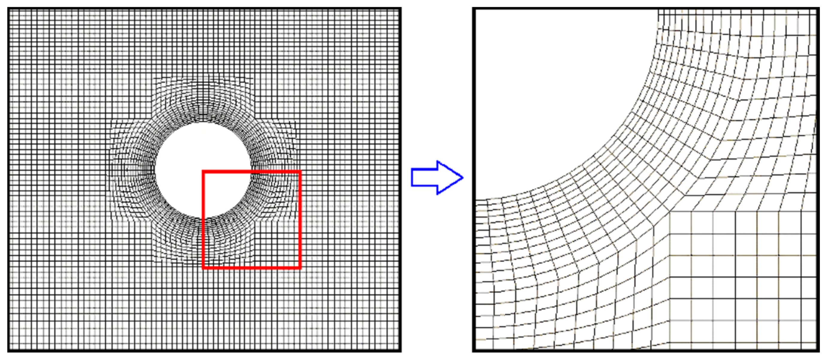
3.1. Numerical Setup

The present viscous numerical simulations are set up by reference to Wu’s (1993) potential analytical study, and a sketch of the computation domain is shown in Figure 4. The axis of the cylinder is placed at the center position in the horizontal direction of the wave tank, and 3 L from the two relaxation zones at the initial time. The radius and the submergence depth of the cylinder are r = 0.1 m and s = 0.3 m, respectively. Two relaxation zones II for damping the radiation waves are arranged at the front and the end of the wave tank, and the length of the two zones is set as 2.5 L. The water depth is d = 4.0 m. The oscillations of the circular cylinder are considered as simple harmonic motions separately in the horizontal and vertical directions. The equations for the oscillatory motions are as follows:

$$\{\begin{array}{l}x(t)=B\sin (\omega t)\\ z(t)=B\sin (\omega t),\end{array}$$

(10)

where B and ω are the oscillation amplitude and the oscillation frequency, respectively. The numerical simulations start from the still water state.

Eight oscillation amplitudes of B/r = 0.20~1.75 and two oscillation frequencies of kr = 0.1 (ω = 3.31 rad/s) and kr = 1.0 (ω = 9.90 rad/s) are adopted in the simulations, where k = ω²/g is the radiation wave number. To study the viscous effects on the hydrodynamic forces, two kinematic viscosity coefficients of υ = 1.0 × 10⁻⁶ (m²/s) and υ = 1.0 × 10⁻⁴ (m²/s) are considered for the liquid phase, and the corresponding real fluids can be considered as water and oil. The corresponding cases are named as the small viscosity cases and the large viscosity cases in the following sections, respectively.

The Keulegan–Carpenter (Kc) number for the present calculation cases can be obtained as follows:

$$\mathrm{Kc}=\frac{UT}{D}=\frac{\pi B}{r},$$

(11)

where U and D are the relative velocity of the fluid and the cylinder diameter, respectively. The Reynolds (Re) number for the present cases can be defined as:

$$\mathrm{Re}=\frac{UD}{\upsilon }=\frac{2B\omega r}{\upsilon }.$$

(12)

The Stokes frequency parameter β proposed by Sarpkaya (1981) [40] for describing flow oscillation characteristics is expressed as:

$$\beta =\frac{\mathrm{Re}}{\mathrm{Kc}}=\frac{2\omega r^2}{\pi \upsilon }.$$

(13)

The above-mentioned parameters for all the calculation cases are listed in

Table 1. Parameters for the simulations.

Case	B/r	Kc	υ = 1.0 × 10−6 (m2/s)		υ = 1.0 × 10−4 (m2/s)
			kr = 0.1	kr = 1.0	kr = 0.1	kr = 1.0
			ω = 3.31 rad/s	ω = 9.90 rad/s	ω = 3.31 rad/s	ω = 9.90 rad/s
			β = 1.0 × 104	β = 3.14 × 104	β = 1.0 × 102	β = 3.14 × 102
			Re	Re	Re	Re
1	0.20	0.63	6.26 × 103	1.98 × 104	6.26 × 10	1.98 × 102
2	0.40	1.26	1.25 × 104	3.96 × 104	1.25 × 102	3.96 × 102
3	0.60	1.88	1.88 × 104	5.94 × 104	1.88 × 102	5.94 × 102
4	0.80	2.51	2.51 × 104	7.92 × 104	2.51 × 102	7.92 × 102
5	1.00	3.14	3.13 × 104	9.90 × 104	3.13 × 102	9.90 × 102
6	1.25	3.93	3.92 × 104	1.24 × 105	3.92 × 102	1.24 × 103
7	1.50	4.71	4.70 × 104	1.49 × 105	4.70 × 102	1.49 × 103
8	1.75	5.50	5.48 × 104	1.73 × 105	5.48 × 102	1.73 × 103

.

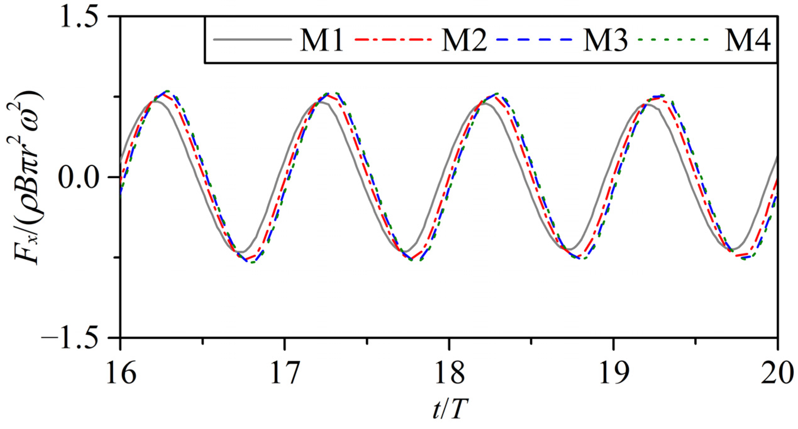
3.2. Grid Dependency Test

Grid dependency tests are investigated by means of the present calculation model for the horizontal-oscillation case with kr = 1.0, B/r = 1.25 and υ = 1 × 10⁻⁶ (m²/s), which is chosen as an example. A typical grid and the refinement of local meshes around the circular cylinder for the simulations are shown in Figure 5. In the case, the inner diameter of the annular refinement region is 1.2 r. In the refinement region, the width of the cells gradually increases in the normal direction of the body surface boundary.

Four groups of computational meshes with different resolutions are utilized for the dependency tests. The numbers for the uniform cells in a wavelength (N-L), the uniform cells in a wave height (N-H), the uniform cells along the cylinder surface (N-S), the gradually changing cells in the radius of the refinement area (N-R), and the total cells (N-T) are listed in

Table 2. Mesh parameters.

Mesh	N-L	N-H	N-S	N-R	N-T
M1	30	6	24	8	2.57 × 104
M2	60	12	60	12	9.46 × 104
M3	100	20	120	24	2.18 × 105
M4	120	24	160	32	3.22 × 105

.

Figure 6 shows the comparisons of the horizontal forces on the circular cylinder with the variable resolution grids for the case of kr = 1.0, B/r = 1.25 and υ = 1 × 10⁻⁶ (m²/s) in the horizontal-oscillation situation. In the figures, ‘F/(ρBπr²ω²)’ represents the non-dimensional hydrodynamic force. The difference can be observed between results at the coarse and the fine meshes. The results by mesh M3 almost coincide with those of mesh M4. It indicates that the fineness of mesh M3 and M4 is sufficient to obtain convergent numerical results. To reduce the computational cost on the premise of ensuring the calculating precision, the mesh type of M3 will be utilized for the calculations in the later sections.

4. Comparison of the Results and Analysis of the Forces and Flow Field

By computing and disposing the forces exerted on the circular cylinder, the hydrodynamic forces from the viscous fluid numerical simulations under different viscosities and two corresponding set of results obtained from two potential flow models are compared in this section. The influential characteristics of the liquid viscosity on the hydrodynamic forces are found from the hydrodynamic forces, the force components, and the phase relations of the forces and motions. The viscous effects are discussed by examining the features of the flow field surrounding the cylinder and analyzing the characteristics of the surface pressure on the cylinder.

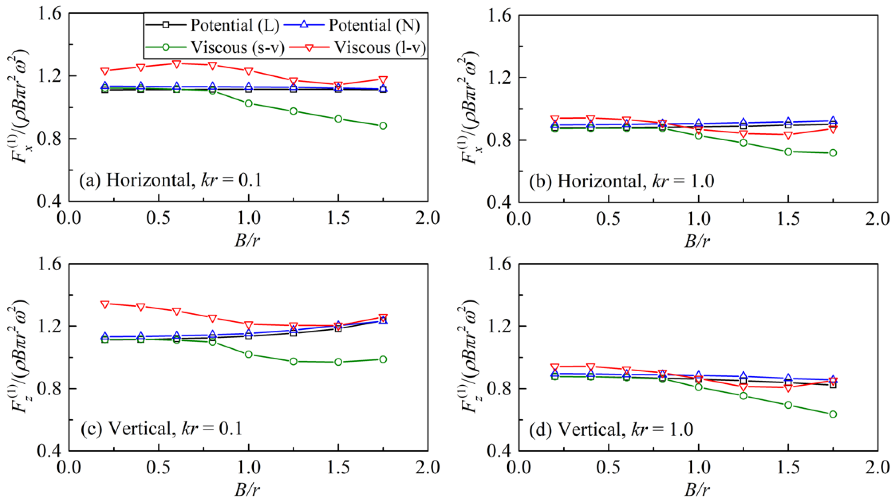
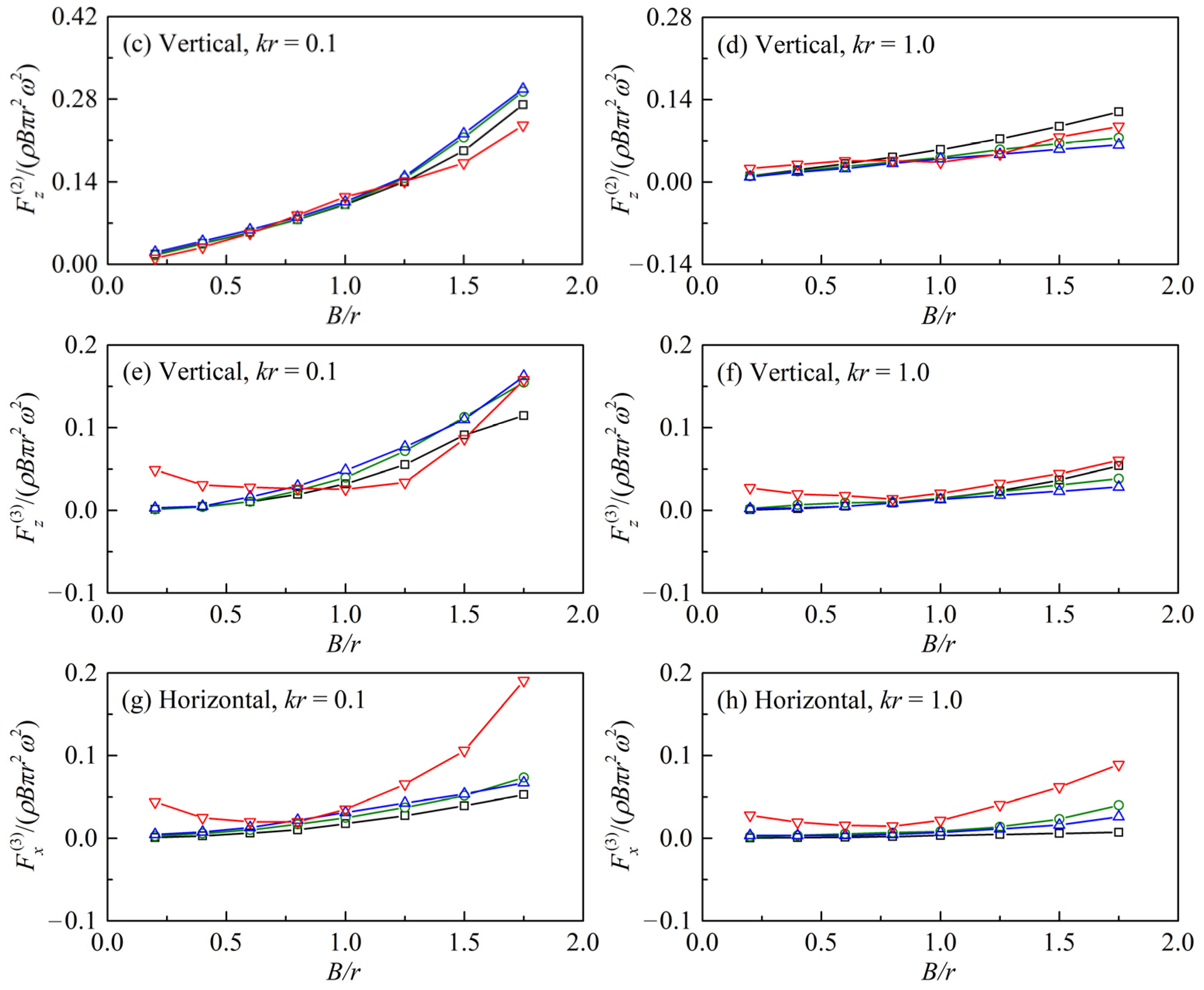
4.1. Hydrodynamic Force Results

The various frequency components of the hydrodynamic forces obtained following Equation (9) in the non-dimensional form of F/(ρBπr²ω²) as a function of B/r are treated as the objects for comparisons. To show the effects of fluid viscosity, flow rotation, and free-surface condition, Wu’s (1993) potential analytical solutions and a set of results obtained numerically using a high-order BEM with a 2-D NWT model are examined [41]. A linearized boundary condition for the free surface and a nonlinear boundary condition for the body surface is taken into account by the former and nonlinear boundary conditions for the free surface and body surface are considered by the latter.

In the following comparisons, ‘horizontal’ and ‘vertical’ refer to the cases that the forced oscillation of a cylinder is in the horizontal direction and in the vertical direction, respectively; the ‘(L)’ and ‘(N)’ in the legends are the linear and nonlinear free-surface conditions, and correspond to Wu’s (1993) potential analytical solutions and the potential numerical results by the higher-order BEM. The ‘(s-v)’ and ‘(l-v)’ refer to viscous numerical results from the small viscosity cases and the large viscosity cases, respectively.

Figure 7 shows the comparisons of the fundamental-frequency hydrodynamic forces along the direction of harmonic motions. The good agreement between the two sets of potential flow solutions indicates the different boundary conditions of the free surface have no obvious influence on the fundamental-frequency hydrodynamic forces. In the small viscosity cases (υ = 1 × 10⁻⁶ (m²/s)), at the small amplitude band (e.g., B/r = 0.20~0.80), the viscous results are generally close to the potential results; however, with the increase of B/r (e.g., B/r = 1.00~1.75), the non-dimensional viscous results gradually become smaller, namely, the gaps between the results from the viscous fluid and potential flow models increase. This indicates that at these large amplitudes, there are significant viscous effects on the fundamental-frequency hydrodynamic forces.

While for the large viscosity cases (υ = 1 × 10⁻⁴ (m²/s)), at the small amplitude band (e.g., B/r = 0.20~0.60), the viscous numerical results become pronouncedly larger than the results from the potential flow models, the non-dimensional hydrodynamic forces firstly gradually decrease with the increase of B/r (e.g., B/r = 0.80~1.25) and then increase (e.g., B/r = 1.50~1.75). These comparative characteristics of the results suggest that the fundamental-frequency hydrodynamic forces in the whole amplitude band are affected dramatically by fluid viscosity and flow rotation.

Figure 8 shows the zero-frequency component ((a), (b)), the double-frequency component ((c), (d)), and the triple-frequency component of the hydrodynamic forces ((e)~(h)) along the direction of harmonic motions. The results for the small viscosity cases (υ = 1 × 10⁻⁶ (m²/s)) are close to the potential results. However, there are different degrees of discrepancies between the viscous results for the large viscosity cases (υ = 1 × 10⁻⁴ (m²/s)) and the other groups of results. So, there are significant viscous effects on the zero-frequency and the high-frequency hydrodynamic forces along the harmonic-motion direction in the cases with the larger liquid viscosity but inconspicuous viscous effects in the cases with the smaller liquid viscosity. The slight discrepancies between the two groups of potential flow solutions are caused by the different free-surface conditions.

Figure 9 shows the zero-frequency ((a), (b)) and the double-frequency vertical hydrodynamic forces ((c), (d)) under harmonic motions in the horizontal direction. In these cases of the cylinder under horizontal harmonic motions, due to the existence of the radiation waves, the mean vertical forces are nonzero values. At the small amplitude band (e.g., (b) B/r = 0.20~0.60), the two groups of viscous results under the different liquid viscosities are very close to the potential results. Nevertheless, with the increase of B/r (e.g., (c) B/r = 0.10~1.75), the varying degrees of gaps among the two sets of viscous results and the potential results emerge in the figures. The gaps between the results under the larger viscosity and the potential flow solutions, by contrast, are larger. This suggests that for the large amplitude band, there are significant viscous effects on the zero-frequency and the double-frequency vertical forces under the horizontal harmonic motions. The effects of the fluid viscosity and flow rotation on the forces are more significant under the larger viscosity. In addition, the different conditions of the free surface are also regarded as the specific reason for the discrepancies between the two groups of potential results.

4.2. Resolution and Phase Relation of Force

To investigate the contributions of each component to the hydrodynamic forces, the pressure and shear forces in different viscosity conditions are compared respectively. The horizontal-oscillation cases with B/r = 0.40, 1.25, and 1.75 are considered as typical examples. The time histories of the pressure forces ((a1), (a2), (a3) for kr = 0.1 and (b1), (b2), (b3) for kr = 1.0) and the viscous shear forces ((c1), (c2), (c3) for kr = 0.1 and (d1), (d2), (d3) for kr = 1.0) on the cylinder from the viscous fluid model (‘(s-v)’ and ‘(l-v)’ in the legends) and the nonlinear potential model (‘(N)’ in the legends) are shown in Figure 10. In the figures, to clearly show the phase difference of the forces, ‘E-N’ and ‘E-s-v’ are used to mark the moments that the pressure forces from the potential model with nonlinear free-surface conditions and the viscous shear forces in the small viscosity cases reach their respective peak values.

The figures show that, for the small oscillation amplitudes (e.g., B/r = 0.40 in (a1) and (b1)), the pressure forces on the cylinder in the viscous fluid cases are almost consistent with the potential flow solutions whether in amplitude value or in phase. As the oscillation amplitude increases (e.g., B/r = 1.25 in (a2) and (b2)), the amplitude values of the pressure forces under the two kinds of viscosities are all less than the potential flow solutions. From the viscous model, the phase of the pressure forces is hysteretic compared with the potential results. This phase-hysteresis phenomenon is more obvious in the large viscosity cases. Specially, as the amplitude exceeds some value, the amplitude values of the pressure forces for the large viscosity cases are larger than the potential results, and those from the small viscosity cases are still smaller than the potential results (e.g., B/r = 1.75 in (a3) and (b3)). There is a more significant phase-hysteresis phenomenon.

In the small viscosity cases, compared with the pressure forces, the viscous shear forces have very a small magnitude. However, the contribution made by the viscous shear forces under the larger liquid viscosity cannot be ignored by the resultant forces. Moreover, a phase-advance phenomenon is evident in all of the viscous fluid cases. More specifically, the phase of the viscous shear forces under large viscosity is advanced compared with the results under small viscosity. It is worth noting that with the 100-fold increase of the liquid viscosity coefficient, the viscous shear forces increase less than 100 times. This is because with the viscosity increases, the thickness of the boundary layer increases, and the normal velocity gradient decreases. According to Equations (7) and (8), the disproportionate increase of the viscous shear forces can be easily understood.

According to the above phase difference of the forces, the relations between the hydrodynamic forces on the cylinder and motion of the cylinder under different liquid viscosities may be different. The horizontal-oscillation cases are considered as examples. The horizontal positions of the cylinder axis as the horizontal forces on the cylinder reach negative ((a), (c)) and positive ((b), (d)) extremums are examined, and the corresponding potential and viscous results are compared in Figure 11. In the figures, ‘x/B’ is a non-dimensional quantity and refers to the axis horizontal positions (x/B = 0.0 is the oscillation center, x/B = −1.0 and 1.0 are the negative and positive oscillation endpoints). For the viscous fluid cases, the representative typical positions of the axis are shifted towards the oscillation center as the amplitude increases. Some phenomena observed from the comparisons in Figure 10 (a1~a3) and (b1~b3) can be intuitively understood. Compared with the potential results, the calculated pressure forces considering viscosity are hysteresis in phase. To be precise, the horizontal forces reach the extremums, which occurs in the process of the cylinder moving from the oscillation endpoint to the center. Furthermore, this phenomenon is more obvious in the large viscosity cases (υ = 1 × 10⁻⁴ (m²/s)). Besides, at small amplitudes (e.g., B/r = 0.20), owing to the larger viscous shear forces, the axis positions under the large liquid viscosity deviate from the other results.

In the above comparisons of the results from the cases with different liquid viscosities, some special physical phenomena are found, and different liquid viscosities have various degrees of influence on the hydrodynamic forces. The reasons for the discrepancies of the different characteristics among the hydrodynamic forces and the viscous-effect mechanisms are analyzed and explained in the next section.

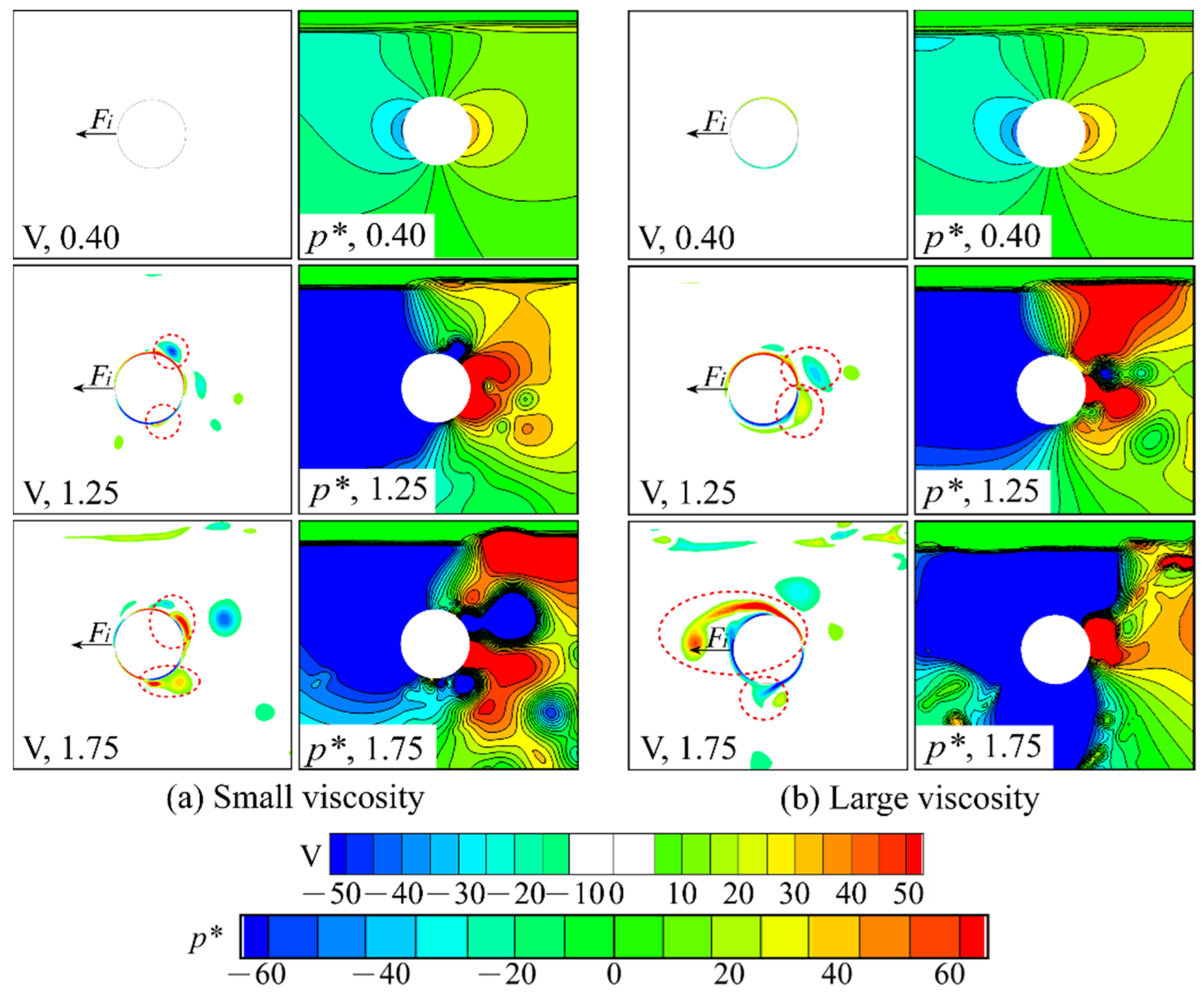
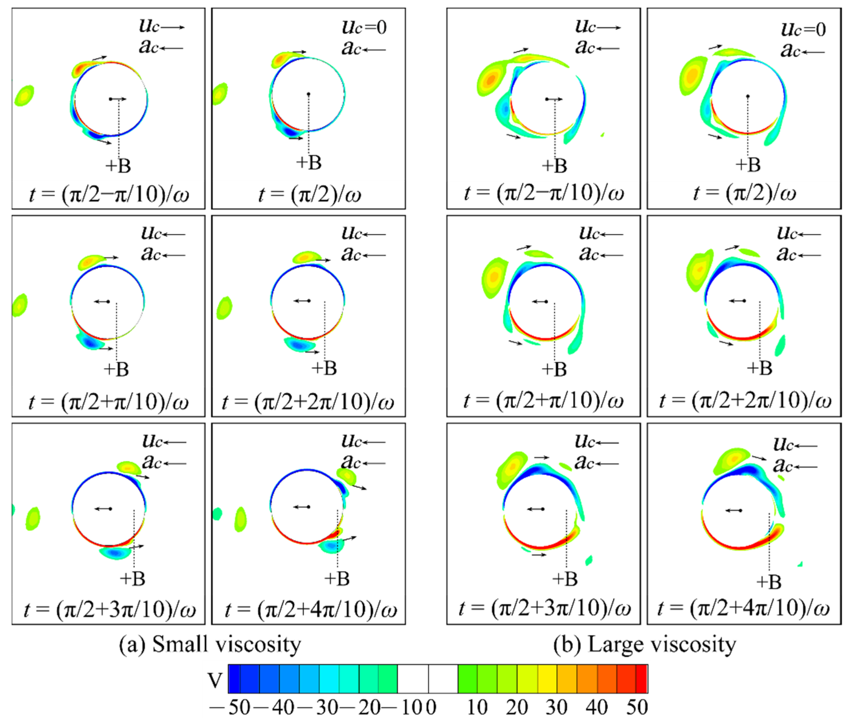
4.3. Viscous Flow Fields around the Cylinder

On the basis of the above comparisons and analysis, some phenomena can already be explained. As shown in Figure 10, under the small viscosity, the viscous shear forces with fairly small values can be ignored. However, considerable contribution to the total hydrodynamic forces is made by the viscous shear forces under the larger liquid viscosity. Thus, for the fundamental-frequency hydrodynamic forces along the harmonic-motion direction, at the small amplitude band (e.g., B/r = 0.20~0.60), the results from the small viscosity cases (υ = 1 × 10⁻⁶ (m²/s)) are close to the corresponding potential solutions, as shown in Figure 7. However, the results from the large viscosity cases (υ = 1 × 10⁻⁴ (m²/s)) are larger than the potential solutions and the viscous results under the smaller liquid viscosity. For the zero-frequency, double-frequency, and triple-frequency hydrodynamic forces along the harmonic-motion direction, the results under the larger liquid viscosity are apparently different from the other groups of results, as shown in Figure 8. Excluding the influence of the linear and non-linear free surface conditions, the larger proportion of the viscous shear forces in the resultant force is another decisive reason. More specifically, the influence of the zero-frequency and the high-frequency components of the shear forces on the hydrodynamic forces is the main cause.

To explain the reasons for the other phenomena, examinations on the flow fields around the cylinder and the surface pressure on the body are carried out. In the following examinations, the horizontal-oscillation cases are considered as typical examples.

The 2-D viscous flow fields, namely, the vorticity fields and the dynamic pressure fields around the circular cylinder, are examined in this section, and the cases with the conditions of kr = 0.1, B/r = 0.40, 1.25, and 1.75 are considered here. Figure 12 shows the distribution of viscous flow fields as the horizontal pressure forces reach the negative extremums. In the labels, V (s⁻¹) and p* (Pa) respectively represent the vorticity and dynamic pressure, and the vorticity can be calculated by:

$$\mathrm{V}=\frac{\partial v}{\partial x}-\frac{\partial u}{\partial z},$$

(14)

where u and v represent the velocity components of fluid in the horizontal and vertical directions, respectively. The numbers in the lower-left corner of the figures are the non-dimensional oscillation amplitude of B/r.

For judging the relative motion trend, the ‘F_i’ with an arrow represents the direction of inertia force as well as the direction of the fluid relative acceleration. From the flow field results, it is seen that in the cases at B/r = 0.40 under the different liquid viscosities, there is no obvious vortex around the cylinder, and an approximated symmetrical pressure distribution at the front and rear of the cylinder. For the B/r = 1.25 and 1.75 cases, the vorticity fields show that some vortices are created from the boundary layer separation and close to the surface, and are distributed on the positive pressure side. For a vortex, its internal pressure is always lower than external far-field pressure according to the fluid dynamics. The pressure fields also show that the pressure at the locations of the vortex formation is lower than the surrounding pressure. In other words, the extreme pressure forces are reduced by the vortex effect compared with the potential flow cases. Despite increasing the amplitude or increasing the fluid viscosity, the vortex strength and the negative pressure area increase, and the proportion of the total forces taken up by the equivalent forces of the vortex effect also increase gradually. Thus, the non-dimensional results of the fundamental-frequency hydrodynamic forces shown in Figure 7 gradually decrease with the increase of the amplitude at B/r = 0.10~1.75 in the small viscosity cases and B/r = 0.80~1.25 in the large viscosity cases.

According to above numerical results shown in Figure 12, affected by wave radiation, the vortices above the cylinder top close to the free surface and below the cylinder display an unsymmetrical distribution. In the cases with harmonic motions in the horizontal direction, the vertical forces consist of the pressure forces and viscous shear forces in the vertical direction. The vertical components of the pressure forces are mostly caused by the asymmetric dynamic pressure distribution on the top half and upper half part of the circumference surface attributed to the wave radiation. Thus, the vortex unsymmetrical distribution has a non-negligible effect on the vertical components of pressure forces, which causes the gaps in the comparisons of the zero-frequency and double-frequency vertical forces in the cases with the horizontal harmonic motions shown in Figure 9. Because the asymmetry of the vortex distribution is more obvious in the flow fields under the larger liquid viscosity, the corresponding results of the non-dimensional forces are obviously different from the other groups of results, as shown is Figure 9.

To describe and analyze the pressure distribution on the circular cylinder surface corresponding to the flow field characteristics, the angle along the circumference of the cylinder is defined in Figure 13. From the preceding results at B/r = 1.75, it can be found that at the moments that the pressure forces reach the negative horizontal extremums, the vortices appear close to the body surface at the circumferential positions with angles of about 60° and 300° in the small viscosity coefficient cases, and about 60°~180° and 240°~270° for the cases with the larger liquid viscosity.

The pressure distribution on the cylinder surface as the pressure forces reach the negative and positive horizontal extremums for the viscous fluid cases under kr = 0.1 at B/r = 0.40 and B/r = 1.75 are shown in Figure 14. The non-dimensional form of dynamic pressure is denoted by p*/(ρBπr²ω²), the θ (deg.) represents the degrees of the circumferential angle. The effects of the vortices close to the body surface on the pressure can be intuitively observed in the figures. The pressure curves are smooth in the small-amplitude cases (without a vortex effect). In the large-amplitude cases, some obvious sags on the curves at the corresponding angles on the circumference of the vortices are observed. For the small viscosity coefficient case of B/r = 1.75, the original positive pressure values under a small amplitude are relatively reduced under the vortex effect (e.g., Figure 14, (a) θ is about 60° and 300°, (b) θ is about 120° and 240°). This leads to the diminution of the curve integration area in the horizontal direction. In the large viscosity coefficient case of B/r = 1.75, although the positive pressure values are still reduced, the negative pressure values are increased under the vortex effect (e.g., Figure 14, (a) θ is about 60°~180° and 240°~270°, (b) θ is about 60°~120° and 270°~300°). The horizontal integration area of the curves actually increases. This condition verifies that in the small viscosity coefficient case of B/r = 1.75, the magnitude of the pressure forces is reduced by the vortex effect; in other words, the amplitude value of the equivalent forces for the vortex effect is comparatively small. However, the amplitude value of the equivalent forces for the vortex effect is considerably larger in the case of B/r = 1.75 under the larger viscosity, and the increase of the pressure-force magnitude is mostly due to the vortex effect. Thus, for the fundamental-frequency hydrodynamic forces along the harmonic-motion direction, at the amplitude band of B/r = 1.50~1.75 (shown in Figure 7), with the increase of the amplitude, the non-dimensional forces always decrease under the smaller liquid viscosity, but gradually decrease firstly and then increase under the larger liquid viscosity.

Figure 15 shows the comparisons of the vorticity fields around the cylinder under different viscosities at some instantaneous positions in one harmonic motion period. The cases of kr = 0.1 with horizontal harmonic motion at B/r = 1.25 are considered as examples here. In the figures, ‘u_c’, ‘a_c’ with arrows and ‘+B’ indicate the motion velocity and its direction of the cylinder, the acceleration and corresponding direction of the cylinder, and the positive direction oscillation endpoint, respectively. The motion power of the vortices is derived from the structural motion, and the figures show that the vortex motion is behind the cylinder, and this hysteresis is more significant in the cases with the larger liquid viscosity. Consequently, compared with the pressure forces of the potential flow solutions, the phase of the equivalent forces for the vortex effect is hysteretic. Thus, the phase of the pressure forces including the vortex effect equivalent forces from the viscous fluid model is also hysteretic compared with the potential results. Due to the more hysteretic vortex motion, the phase hysteresis phenomenon of the pressure forces in the cases with the larger liquid viscosity is more obvious.

To explain the reason for the phase-advance phenomenon of the viscous shear forces as mentioned above, the distribution of flow streamlines around the cylinder at the instants when the horizontal viscous shear forces reach the positive extremums are investigated. The cases with horizontal harmonic motion of kr = 0.1 at B/r = 1.25 are considered as typical examples, and the comparison of the flow field results is shown in Figure 16, where ‘C’ represents the horizontal oscillation center. The figures show that at the typical instant ((t = (π/2 + 3π/8)/ω)), the axis of the circular cylinder in the small viscosity coefficient case (υ = 1 × 10⁻⁶ (m²/s)) is relatively closer to the oscillation center and the cylinder instantaneous velocity is close to the maximum value of the simple harmonic motion velocity. At the typical instant (t = (π/2 + π/9)/ω), in the large viscosity coefficient case (υ = 1 × 10⁻⁴ (m²/s)), the cylinder is moving from the oscillation endpoint to the center and relatively further to the oscillation center. Due to the stronger hysteresis of the fluid motion, the fluid velocity is still in the opposite direction to the cylinder motion. In the process, the relative velocity between the fluid and the structure reaches its maximum values, and the viscous shear forces reach the extreme values. Thus, compared with the results for the small viscosity coefficient cases, the phase advance phenomenon of the viscous shear forces is obvious under the larger liquid viscosity.

To simplify the calculation, the hydrodynamic force on a moving structure according to the potential flow theory can be expressed as:

$$F_R=-ma(t)-bu(t),$$

(15)

where m, a(t), b, and u(t) represent the added mass, acceleration of structure motion, radiation damping, and velocity of structure motion, respectively. Regarding the forces on the oscillating cylinder underwater with a deep submerged depth, b in Equation (15) tends to be zero. Therefore, the resultant forces on the cylinder are almost in the same phase of the harmonic motion. However, in the simulations based on the viscous fluid theory, the situation is quite different.

From the different curve shapes in Figure 11, it can be seen that the relations between the extreme forces and the cylinder positions are different under different viscosities based on different theories. Through the above analysis on the flow field distribution, there are viscous effects on the relations between the hydrodynamic force and the cylinder movement. For one thing, the vortex equivalent forces are hysteretic in phase compared with the pressure forces in the potential flow solutions. This leads to the different levels of hysteresis for the pressure forces under different liquid viscosities. For another thing, under the larger viscosity, viscous shear forces provide a larger contribution. Thus, the horizontal forces reach the extremums when the cylinder moves from the oscillation endpoint to the center.

5. Conclusions

The liquid viscosity effects on the hydrodynamic forces on a submerged circular cylinder underwater in forced oscillatory motion were examined by viscous fluid simulations considering two kinematic viscosity coefficients in this study. It was found that due to the different mechanisms and various degrees of viscous effects, there are different characteristics for the various frequency components of hydrodynamic forces on the cylinder under different liquid viscosities.

The conclusions drawn from this study are summarized as follows:

• There is a significant difference among the groups of viscous fluid results and potential flow solutions for the fundamental frequency hydrodynamic forces along the harmonic motion direction. The reasons for the phenomenon are the different proportions of the viscous shear forces in the resultant forces and the different levels of vortex effects on the pressure forces.
• Because viscous shear forces take up a larger proportion of the resultant force, the zero-frequency, double-frequency, and triple-frequency hydrodynamic forces at the large amplitudes along the harmonic motion direction under the larger viscosity are larger than the other groups of results.
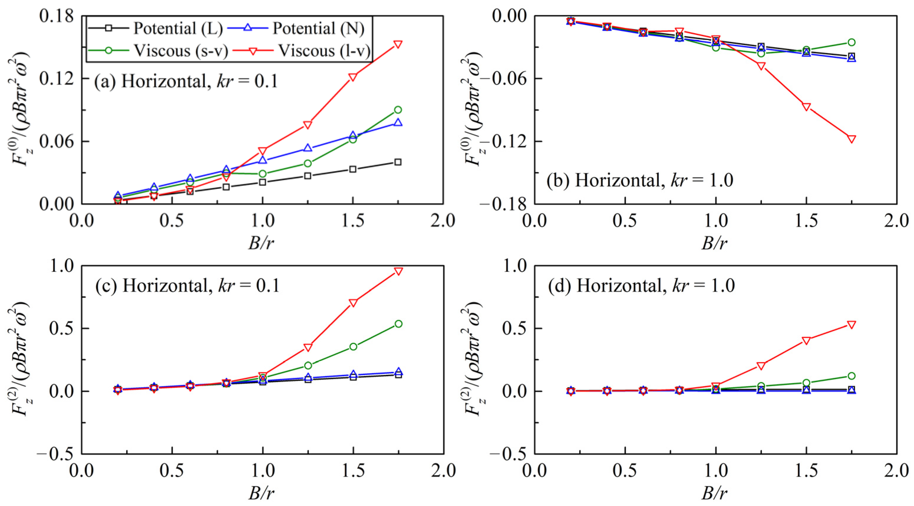
• The wave radiation caused the asymmetric distribution of the vortices in the vertical direction above and below the cylinder, and influences the pressure forces in the cases with horizontal harmonic motions. This reason results in the gaps among the results of the zero-frequency and the double-frequency vertical forces based on the different theories and various viscosities.
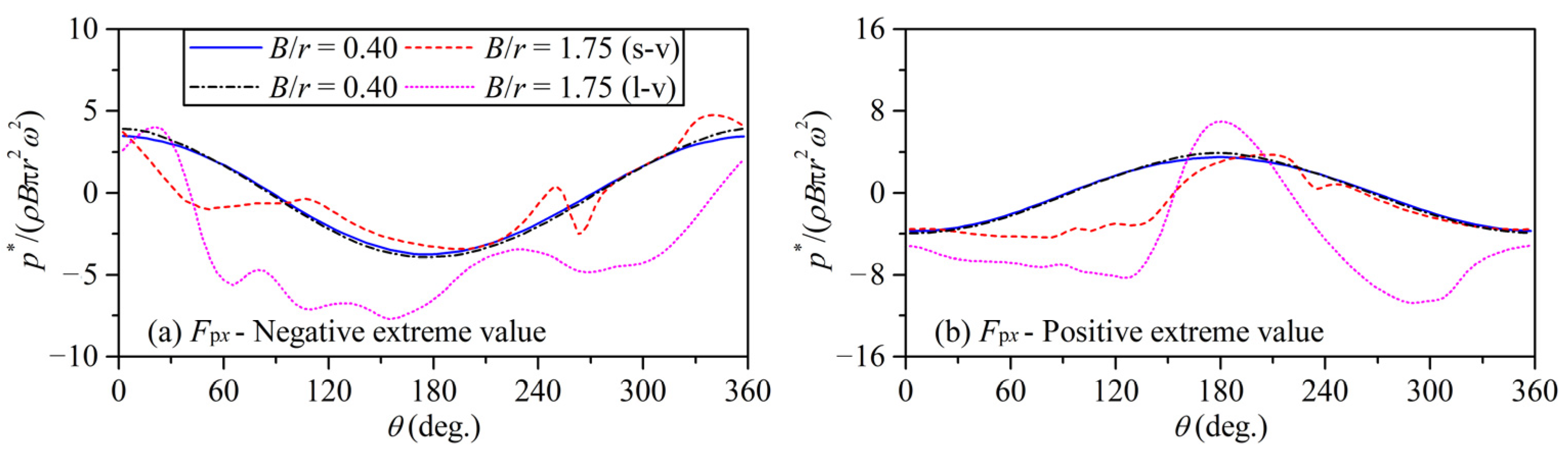
• Because the vortex motion is behind the cylinder motion, and the hysteresis is more significant under the larger liquid viscosity, the phase-hysteresis phenomenon in varying degrees is shown from the comparisons of the pressure forces among the groups of viscous fluid results and potential flow solutions.
• Due to the stronger hysteresis of the large-viscosity fluid flow, the viscous shear forces reach their extremums at the moment the fluid velocity remains in the opposite direction of the cylinder motion. Hence, compared with the results under the small liquid viscosity, the phase-advance phenomenon of the viscous shear forces is obvious under the larger liquid viscosity.
• Under the larger liquid viscosity, the more significant phase-hysteresis of the pressure forces and the larger contribution provided by the viscous shear forces results in the horizontal forces reaching the extremums at a certain moment when the cylinder moves from the oscillation endpoint to the center.

The above conclusions may have practical guiding significance to the scientific design and safety production of some ocean engineering structures, such as major structures of cross-sea submerged floating tunnels, components of floating wave energy generators, underwater structures of platforms and production risers, etc.

In this article, the authors reaffirmed that the conclusions from this work are restricted in 2-D space. To identify the actual 2-D to 3-D scaling effects, follow-up 3-D studies will be carried out in the future.

References

1. Wu, G.X. Hydrodynamic forces on a submerged circular cylinder undergoing large-amplitude motion. J. Fluid Mech. 1993, 254, 41–58. [Google Scholar] [CrossRef]
2. Rahman, M.; Bhatta, D.D. Evaluation of added mass and damping coefficient of an oscillating circular cylinder. Appl. Math. Model. 1993, 17, 70–79. [Google Scholar] [CrossRef]
3. Tyvand, P.A.; Miloh, T. Free-surface flow due to impulsive motion of a submerged circular cylinder. J. Fluid Mech. 1995, 286, 67–101. [Google Scholar] [CrossRef]
4. Tyvand, P.A.; Miloh, T. Free-surface flow generated by a small submerged circular cylinder starting from rest. J. Fluid Mech. 1995, 286, 103–116. [Google Scholar] [CrossRef]
5. Wu, G.X.; Eatock Taylor, R. Time stepping solutions of the two-dimensional non-linear wave radiation problem. Ocean Eng. 1995, 22, 785–798. [Google Scholar] [CrossRef]
6. Greenhow, M.; Moyo, S. Water entry and exit of horizontal circular cylinders. Philos. Trans. R. Soc. 1997, A355, 551–563. [Google Scholar] [CrossRef]
7. Liu, Y.M.; Zhu, Q.; Yue, D.K.P. Nonlinear radiated and diffracted waves due to the motions of a submerged circular cylinder. J. Fluid Mech. 1999, 382, 263–282. [Google Scholar] [CrossRef]
8. Kent, C.P.; Choi, W. An explicit formulation for the evolution of nonlinear surface waves interacting with a submerged body. Int. J. Numer. Methods Fluids 2007, 55, 1019–1038. [Google Scholar] [CrossRef]
9. Guerber, E.; Benoit, M.; Grilli, S.T.; Buvat, C. Modeling of fully nonlinear wave interactions with moving submerged structures. In Proceedings of the International Offshore and Polar Engineering Conference, Beijing, China, 20–25 June 2010; pp. 529–536. Available online: https://www.mendeley.com/catalogue/6952d253-6fcb-3338-b04f-b515f1db78b3/ (accessed on 8 August 2021).
10. Guerber, E.; Benoit, M.; Grilli, S.T.; Buvat, C. A fully nonlinear implicit model for wave interactions with submerged structures in forced or free motion. Eng. Anal. Bound. Elem. 2012, 36, 1151–1163. [Google Scholar] [CrossRef] [Green Version]
11. Guilmineau, E.; Queutey, P. A numerical simulation of vortex shedding from an oscillating circular cylinder. J. Fluids Struct. 2002, 16, 773–794. [Google Scholar] [CrossRef]
12. Yang, S.J.; Chang, T.R.; Fu, W.S. Numerical simulation of flow structures around an oscillating rectangular cylinder in a channel flow. Comput. Mech. 2005, 35, 342–351. [Google Scholar] [CrossRef]
13. Wu, Y.L.; Shu, C. Application of local DFD method to simulate unsteady flows around an oscillating circular cylinder. Int. J. Numer. Methods Fluids 2008, 58, 1223–1236. [Google Scholar] [CrossRef]
14. Pham, A.H.; Lee, C.Y.; Seo, J.H.; Chun, H.H.; Kim, H.J.; Yoon, H.S.; Kim, J.H.; Park, D.W.; Park, I.R. Laminar flow past an oscillating circular cylinder in cross flow. J. Mar. Sci. Technol.-Taiwan 2010, 18, 361–368. [Google Scholar] [CrossRef]
15. Peter, S.; De, A.K. Characteristics of the wake behind a transversely oscillating cylinder near a wall. J. Fluids Eng. 2017, 139, 031201. [Google Scholar] [CrossRef]
16. Mittal, S. Three-dimensional instabilities in flow past a rotating cylinder. J. Appl. Mech. 2004, 71, 89–95. [Google Scholar] [CrossRef] [Green Version]
17. Rao, A.; Leontini, J.; Thompson, M.C.; Hourigan, K. Three-dimensionality in the wake of a rotating cylinder in a uniform flow. J. Fluid Mech. 2013, 717, 1–29. [Google Scholar] [CrossRef]
18. Wang, Q.; Kou, Y.F.; Zhu, R.Q.; Chen, H. 3D effects on vortex-shedding flow and hydrodynamic coefficients of a vertically oscillating cylinder with a bottom-attached disk. China Ocean Eng. 2017, 31, 428–437. [Google Scholar] [CrossRef]
19. Jacono, D.L.; Bourguet, R.; Thompson, M.C.; Leontini, J.S. Three-dimensional mode selection of the flow past a rotating and inline oscillating cylinder. J. Fluid Mech. 2018, 855, R3. [Google Scholar] [CrossRef]
20. Teng, B.; Mao, H.F.; Lu, L. Numerical simulation of nonlinear water wave action on submerged horizontal circular cylinder. In Proceedings of the Asia-Pacific Workshop on Marine Hydrodynamics, Vladivostok, Russia, 9–13 September 2014; Available online: http://ir.nsfc.gov.cn/handle/00001903-5/408901 (accessed on 8 August 2021).
21. Teng, B.; Mao, H.F.; Lu, L. Viscous effects on wave forces on a submerged horizontal circular cylinder. China Ocean Eng. 2018, 32, 245–255. [Google Scholar] [CrossRef]
22. Jiang, S.C.; Teng, B.; Bai, W.; Gou, Y. Numerical simulation of coupling effect between ship motion and liquid sloshing under wave action. Ocean Eng. 2015, 108, 140–454. [Google Scholar] [CrossRef]
23. Chen, L.F.; Sun, L.; Zhang, J.; Hillis, A.J.; Plummer, A.R. Numerical study of roll motion of a 2-D floating structure in viscous flow. J. Hydrodyn. 2016, 28, 544–563. [Google Scholar] [CrossRef] [Green Version]
24. Gao, J.L.; Zang, J.; Chen, L.F.; Chen, Q.; Ding, H.Y.; Liu, Y.Y. On hydrodynamic characteristics of gap resonance between two fixed bodies in close proximity. Ocean Eng. 2019, 173, 28–44. [Google Scholar] [CrossRef]
25. Chen, L.F.; Taylor, P.H.; Draper, S.; Wolgamot, H. 3-D numerical modelling of greenwater loading on fixed ship-shaped FPSOs. J. Fluids Struct. 2019, 84, 283–301. [Google Scholar] [CrossRef]
26. Teng, B.; Mao, H.F.; Ning, D.Z.; Zhang, C.W. Viscous numerical examination of hydrodynamic forces on a submerged horizontal circular cylinder undergoing forced oscillation. J. Hydrodyn. 2019, 31, 887–899. [Google Scholar] [CrossRef]
27. Hsiao, Y.; Tsai, C.L.; Chen, Y.L.; Wu, H.L.; Hsiao, S.C. Simulation of wave-current interaction with a sinusoidal bottom using OpenFOAM. Appl. Ocean Res. 2020, 94, 101998. [Google Scholar] [CrossRef]
28. Lu, L.; Tan, L.; Zhou, Z.B. Two-dimensional numerical study of gap resonance coupling with motions of floating body moored close to a bottom- mounted wall. Phys. Fluids 2020, 32, 092101. [Google Scholar] [CrossRef]
29. Gao, J.L.; He, Z.W.; Zang, J.; Chen, Q.; Ding, H.Y.; Wang, G. Topographic effects on wave resonance in the narrow gap between fixed box and vertical wall. Ocean Eng. 2019, 180, 97–107. [Google Scholar] [CrossRef]
30. Gao, J.L.; Zhou, X.J.; Zhou, L.; Zang, J.; Chen, H.Z. Numerical investigation on effects of fringing reefs on low-frequency oscillations within a harbor. Ocean Eng. 2019, 172, 86–95. [Google Scholar] [CrossRef]
31. Gao, J.L.; He, Z.W.; Zang, J.; Chen, Q.; Ding, H.Y.; Wang, G. Numerical investigations of wave loads on fixed box in front of vertical wall with a narrow gap under wave actions. Ocean Eng. 2020, 206, 107–323. [Google Scholar] [CrossRef]
32. Zhuang, Y.; Wan, D.C. Numerical simulation of ship motion fully coupled with sloshing tanks by naoe-FOAM-SJTU solver. Eng. Comput. 2019, 36, 2787–2810. [Google Scholar] [CrossRef]
33. Chen, X.; Zhou, Y.L.; Wan, D.C. Numerical study of 3-D liquid sloshing in an elastic tank by MPS-FEM coupled method. J. Ship Res. 2019, 63, 143–153. [Google Scholar] [CrossRef] [Green Version]
34. Liu, Z.H.; Zhuang, Y.; Wan, D.C. Numerical Study of Focused Wave Interactions with a Single-Point Moored Hemispherical-Bottomed Buoy. Int. J. Offshore Polar Eng. 2020, 30, 53–61. [Google Scholar] [CrossRef]
35. Chen, H.F.; Zou, Q.P. Effects of following and opposing vertical current shear on nonlinear wave interactions. Appl. Ocean Res. 2019, 89, 23–25. [Google Scholar] [CrossRef]
36. Weller, H.G.; Tabor, G.; Jasak, H.; Fureby, C. A tensorial approach to computational continuum mechanics using object oriented techniques. J. Comput. Phys. 1998, 12, 620–631. [Google Scholar] [CrossRef]
37. Jacobsen, N.G.; Fuhrman, D.R.; Fredsøe, J. A wave generation toolbox for the open-source CFD library: OpenFOAM. Int. J. Numer. Methods Fluids 2012, 70, 1073–1088. [Google Scholar] [CrossRef]
38. Chaplin, J.R. Non-linear forces on a horizontal cylinder beneath waves. J. Fluid Mech. 1984, 147, 449–464. [Google Scholar] [CrossRef]
39. Fenton, J.D. A fifth-order Stokes theory for steady waves. J. Waterw. Port Coast. Ocean Eng. 1985, 111, 216–234. [Google Scholar] [CrossRef] [Green Version]
40. Sarpkaya, T.; Isaacson, M.; Wehausen, J.V. Mechanics of Wave Forces on Offshore Structures. J. Appl. Mech. 1982, 49, 466–467. [Google Scholar] [CrossRef]
41. Zhou, B.Z.; Ning, D.Z.; Teng, B.; Song, W.H. The numerical simulation of fully nonlinear deep-water waves. Acta Oceanol. Sin. 2011, 33, 27–35. [Google Scholar]
Figure 1. Sketch of the boundaries and relaxation zones for the 2-D numerical wave tank.
Symmetry 13 01806 g001
Figure 2. Sketch of the computational domain for a fixed horizontal circular cylinder completely submerged under wave action.
Symmetry 13 01806 g002
Figure 3. The comparisons of the horizontal and the vertical forces at a variety of A/r. (a) is the horizontal forces on the cylinder; (b) is the vertical forces on the cylinder.
Symmetry 13 01806 g003
Figure 4. Sketch of the computation domain for a horizontal cylinder in oscillatory motion underwater.
Symmetry 13 01806 g004
Figure 5. Typical grid and local mesh refinement around the circular cylinder for the simulations.
Symmetry 13 01806 g005
Figure 6. Time histories of the horizontal forces with variable resolution grids (kr = 1.0, B/r = 1.25, υ = 1 × 10⁻⁶ (m2/s)).
Symmetry 13 01806 g006
Figure 7. Fundamental-frequency hydrodynamic forces along the harmonic-motion direction. (a) is the fundamental-frequency horizontal forces as functions of B/r at kr = 0.1 under horizontal oscillatory motions; (b) is the fundamental-frequency horizontal forces as functions of B/r at kr = 1.0 under horizontal oscillatory motions; (c) is the fundamental-frequency vertical forces as functions of B/r at kr = 0.1 under vertical oscillatory motions; (d) is the fundamental-frequency vertical forces as functions of B/r at kr = 1.0 under vertical oscillatory motions.
Symmetry 13 01806 g007
Figure 8. Zero-frequency, double-frequency, and triple-frequency hydrodynamic forces in the harmonic-motion direction. (a) is the zero-frequency vertical forces as functions of B/r at kr = 0.1 under vertical oscillatory motions; (b) is the zero-frequency vertical forces as functions of B/r at kr = 1.0 under vertical oscillatory motions; (c) is the double-frequency vertical forces as functions of B/r at kr = 0.1 under vertical oscillatory motions; (d) is the double-frequency vertical forces as functions of B/r at kr = 1.0 under vertical oscillatory motions; (e) is the triple-frequency vertical forces as functions of B/r at kr = 0.1 under vertical oscillatory motions; (f) is the triple-frequency vertical forces as functions of B/r at kr = 1.0 under vertical oscillatory motions; (g) is the triple-frequency horizontal forces as functions of B/r at kr = 0.1 under horizontal oscillatory motions; (h) is the triple-frequency horizontal forces as functions of B/r at kr = 1.0 under horizontal oscillatory motions.
Symmetry 13 01806 g008aSymmetry 13 01806 g008b
Figure 9. Zero-frequency and the double-frequency vertical hydrodynamic forces under horizontal harmonic motion. (a) is the zero-frequency vertical forces as functions of B/r at kr = 0.1 under horizontal oscillatory motions; (b) is the zero-frequency vertical forces as functions of B/r at kr = 1.0 under horizontal oscillatory motions; (c) is the double-frequency vertical forces as functions of B/r at kr = 0.1 under horizontal oscillatory motions; (d) is the double-frequency vertical forces as functions of B/r at kr = 1.0 under horizontal oscillatory motions.
Symmetry 13 01806 g009
Figure 10. Comparisons of the magnitude and phase of the force components (B/r = 0.40, 1.25, and 1.75). (a1, b1, c1) are the comparisons of pressure forces for B/r = 0.40, 1.25, and 1.75 at kr = 0.1, respectively; (a2, b2, c3) are the comparisons of pressure forces for B/r = 0.40, 1.25, and 1.75 at kr = 1.0, respectively; (a3, b3, c3) are the comparisons of viscous shear forces for B/r = 0.40, 1.25, and 1.75 at kr = 0.1, respectively; (d1, d2, d3) are the comparisons of viscous shear forces for B/r = 0.40, 1.25, and 1.75 at kr = 1.0, respectively.
Symmetry 13 01806 g010
Figure 11. Horizontal positions of the cylinder axis as the horizontal forces reach extremums. (a) is the cylinder positions as functions of B/r when the horizontal forces reach the negative extremums at kr = 0.1; (b) is the cylinder positions as functions of B/r when the horizontal forces reach the positive extremums at kr = 0.1; (c) is the cylinder positions as functions of B/r when the horizontal forces reach the negative extremums at kr = 1.0; (d) is the cylinder positions as functions of B/r when the horizontal forces reach the positive extremums at kr = 1.0.
Symmetry 13 01806 g011
Figure 12. Vorticity and pressure fields around the cylinder (B/r = 0.40, 1.25, and 1.75). (a) is the vorticity fields and the pressure fields for B/r = 0.40, 1.25, and 1.75 at kr = 0.1 under the smaller liquid viscosity, respectively; (b) is the vorticity fields and the pressure fields for B/r = 0.40, 1.25, and 1.75 at kr = 0.1 under the larger liquid viscosity, respectively.
Symmetry 13 01806 g012
Figure 13. The angle on the circumference.
Symmetry 13 01806 g013
Figure 14. Pressure distribution on the cylinder as the pressure forces reach the horizontal extremums. (a) is the dynamic pressure at the circumferential angles for B/r = 0.40 and 1.75 at kr = 0.1 as the horizontal pressure forces reach the negative extremums under the two viscosities, respectively; (b) is the dynamic pressure at the circumferential angles for B/r = 0.40 and 1.75 at kr = 0.1 as the horizontal pressure forces reach the positive extremums under the two viscosities, respectively.
Symmetry 13 01806 g014
Figure 15. Vorticity fields around the cylinder at some instantaneous positions in an oscillating period (kr = 0.1, B/r = 1.25). (a) is the relative movement trends of the cylinder and the vortices for B/r = 1.25 at kr = 0.1 under the smaller liquid viscosity; (b) is the relative movement trends of the cylinder and the vortices for B/r = 1.25 at kr = 0.1 under the smaller liquid viscosity under the larger liquid viscosity.
Symmetry 13 01806 g015
Figure 16. Comparison of the streamline distribution under different liquid viscosities (kr = 0.1, B/r = 1.25). (a) is the streamline distribution for B/r = 1.25 at kr = 0.1 as the horizontal viscous shear forces reach the positive extremums under the smaller liquid viscosity; (b) is the streamline distribution for B/r = 1.25 at kr = 0.1 as the horizontal viscous shear forces reach the positive extremums under the larger liquid viscosity.
Symmetry 13 01806 g016