On the Time Distribution of Supernova Antineutrino Flux

Abstract

Neutrino leptonic flavor symmetry violation is the only evidence for physics beyond the standard model. Much of what we have learned on these particles is derived from the study of their natural sources, such as the Sun or core-collapse supernovae. Neutrino emission from supernovae is particularly interesting and leptonic flavor transformations in supernova neutrinos have attracted a lot of theoretical attention. Unfortunately, the emission of core-collapse supernovae is not fully understood: thus, an inescapable preliminary step to progress is to improve on that, and future neutrino observations can help. One pressing and answerable question concerns the time distribution of the supernova anti-neutrino events. We propose a class of models of the time distribution that describe emission curves similar to those theoretically expected and consistent with available observations from the data of supernova SN1987A. They have the advantages of being motivated on physical bases and easy to interpret; they are flexible and adaptable to the results of the observations from a future galactic supernova. Important general characteristics of these models are the presence of an initial ramp and that a significant portion of the signal is in the first second of the emission.

1. Introduction

Of the known particles, neutrinos are by far the most mysterious. Neutrino flavor transformations—a phenomenon more commonly known as neutrino oscillations—show that the flavor symmetry of leptons is violated. This phenomenon is the only observational evidence that the standard model of elementary particles is incomplete and was awarded the 2015 Nobel Prize in Physics. Much of what we have learned about neutrinos comes from studying natural sources, such as those recognized by the 2002 Nobel Prize in Physics: The Sun and core-collapse supernovae. In the present work, we investigate the latter source of neutrinos, which is still poorly understood.

Supernovae are a rare astronomical phenomenon, known to mankind for millennia, consisting of a new and very bright star suddenly appearing in the sky. Astrophysics has shown that supernovae play a very important role in the economy of the cosmos, marking the last moments of stellar life and allowing the production and redistribution of chemical elements in the interstellar environment [1,2,3,4,5,6,7,8].

Decades-long discussion about their internal mechanism has made it clear that a specific kind of supernova occurs as a result of a gravitational collapse, which leads to the formation of compact stellar remnants accompanied by a brief and very intense neutrino emission [9,10,11,12,13,14,15,16,17,18,19,20,21,22], and likely by a burst of gravitational waves [23,24,25,26,27,28] (it is now widely accepted that a supernova explosion is an intrinsic multidimensional phenomenon, i.e., essential deviations from the spherical symmetry, with three-dimensional features crucial for triggering an explosion [16,19,29,30]). In this paper, we will discuss neutrino emission from this type of supernovae, which is observable in terrestrial detectors if the supernova occurs in our galaxy, and which is the main diagnostics of events following core collapse.

The only direct observation that we have of the crucial moments of the gravitational collapse is that of supernova 1987A in the Large Magellanic Cloud, thanks to the observation of neutrinos [31,32,33,34,35]. On one hand, the detection made it possible to assess the overall correctness of the current paradigm of neutrino-driven explosion, dating back to the 1960s [36,37,38,39,40], as confirmed by various analyses of the data—see e.g., [41,42,43,44]. On the other hand, however, many important points remain unclear, mostly because of the very few neutrino observed.

In light of these considerations, being able to have observational information would not only be welcome, but actually necessary. It is indeed fair to ask:

What do we know for sure about the various phases of gravitational collapse?

How to learn more using neutrino observations?

In this paper, we will focus on what we can learn from observing electron antineutrinos, which are the ones that give the main signal in conventional, large terrestrial detectors: water or hydrocarbons—see e.g., [45] for a recent review. Although the explosion of a galactic supernova is not a frequent process [46], thanks to the SN1987A data, we are confident that future observations of this type will be possible and significant. Based on similar considerations, new experiments have been equipped to study this channel, and are ready to collect important data statistics. This applies to Super–Kamiokande [47], which has recently upgraded to observe this channel even better [48,49], and partly also to IceCube [50]. The latter will be able to observe the temporal evolution of the signal [50], which is one key point to be clarified through observations. With these considerations in mind, we will present new and convenient models with a physical basis for describing expectations, discussing their motivations and illustrating a few selected applications.

We begin by reviewing the only observations available to date, those of the supernova SN1987A, outlining the progress made in their discussion and understanding, and focusing on the points that remain less well defined and unresolved.

2. Open Issues after Supernova 1987A

The first supernova observed in 1987 (SN1987A) is currently the only occasion when we have been able to directly verify our ideas about the chain of events that occur at key moments in the gravitational collapse. In fact, three neutrino telescopes (or detector), Kamiokande-II, IMB and Baksan [31,33,35] reported observations compatible with this event.

After the enthusiasm of the time, followed by a Nobel Prize awarded to one of the telescopes that detected the neutrino signal, Kamiokande-II, and some rather cautious analyses of the telescope data, summarised in the book “Neutrino Astrophysics” [41], this was followed by numerous comments, critical discussions, and even some doubts. In these subsequent discussions, the following aspects were highlighted:

• that the supernova precursor did not fit fully expectations, and perhaps was non-standard, with unexpected implications;
• that the neutron star had not been observed, even casting a shadow over the significance of the observed events;
• that the observed neutrino events were more directional than expected—directed from the supernova forward-raising similar concerns as in the previous point;
• that also, their average energies were lower than those calculated, perhaps indicating an instrumental problem;
• that the comparability of the energy spectra of Kamiokande-II, IMB and Baksan was not entirely clear;
• that another neutrino detector saw 5 unexpected events [51,52] (for gravitational observatories see [53]), which could be thought of as indications of multiple emission phases and/or substantial deviations from the standard paradigm.

See, e.g., [54] for a summary of the discussion about 10 years ago; here, we present the progress in the discussion of the previous points.

• There is a growing consensus towards the idea that the precursor could have been a two-star system that had recently merged, although it is not clear whether this impacts expectations about core collapse and neutrinos significantly.
• In recent times, the search for the neutron star—which we expected as a result of gravitational collapse—has been guided by the 3D magneto-hydrodynamics model of Miceli and Orlando [55]. This indicated a zone obscured by dust and gas, apparently setting it on the path to success [56,57].
• The direction of the neutrino events, studied e.g., in Ref. [58], seems less problematic than occasionally claimed.
• It has been widely recognized that the theoretical uncertainties in the mean energies are much larger than those estimated in the past, and therefore, it is not currently claimed that there is any serious incompatibility with the theory.
• A complete and systematic study of the energy spectra has verified the compatibility of the energy spectra and confirmed the stability and substantial validity [44] of a standard interpretation, as the one initially summarized by Bahcall. There is a well-defined region of the parameter space that allows the interpretation of the events as due to gravity collapse, as being due to a non-atypical gravitational collapse; the average energy of the antineutrinos is ${\overline{E}}_{\nu }=12 \mathrm{M}\mathrm{e}\mathrm{V}$ and the total radiated energy is of the order of $5\times {10}^{52} \mathrm{erg}$, with errors of 10% and 30%, respectively.
• The only problem that remains unsolved is the meaning of the 5 low-energy events seen by the Mont Blanc/LSD detector [51], which precede those seen by the other three detectors, and which do not seem easy to attribute to the supernova.

In addition, an intense debate about neutrino flavor transformation in the supernova has sparked off particle physics [59,60,61], and not yet come to a complete conclusion—for some extensive reviews of the state of the art, see, e.g., [62,63,64,65,66,67]. One of the main points of discussion is focused on the so-called self-induced neutrino collective oscillations, a phenomenon of a non-linear nature, due to the fact that neutrinos propagate in a medium containing and composed of neutrinos. The study of these situations requires very demanding numerical analyses, and it is not clear whether the approximations used (on neutrino spectra, on spherical or axial geometries, etc.) for the theoretical investigation are realistic or not. For this reason, it is not possible to consider the discussion of these effects concluded or completed to date. Here, we will simply refer to the description of the standard and well-known Mikheyev–Smirnov–Wolfenstein (MSW) effect [68,69] in the context of the intense neutrino emission that takes place with a core-collapse supernova, but this not the only issue that has been discussed. In particular, there has been a great deal of interest in whether or not these types of transformations are crucial for data analysis of SN1987A events [70,71]. The current opinion, as discussed more fully below, is negative [72]. The question of whether these transformations will play a significant role in a future supernova has also been discussed [73], but generally limited to the study of time-integrated spectra (fluence)—see, for example, [74,75]. We will come back to the issue of oscillations in the next section.

On the whole, a minimal interpretation is corroborated: that a neutrino emission due to a gravitational collapse, not too different from the standard one, was indeed observed, followed by the explosion of a supernova and the formation of a compact star. In this light, it is interesting to consider the point originally made by Loredo and Lamb [42], and then confirmed by an independent analysis by Pagliaroli, Vissani, Costantini and Ianni [43]: the interpretation of the time series data suggests that there was an initial phase of very high luminosity (see also Section 5.2). This result is considered interesting, especially because it agrees well with the theoretical expectations about the radiation emission and the supernova explosion. However, it can hardly be considered as a proof, as its significance does not go beyond $2\mathsf{\sigma }$–$3\mathsf{\sigma }$ [42,43].

All this leads one to believe that a precise measurement of the first moments of neutrino emission would be very important or essential in order to make significant progress in understanding the explosion. Therefore, being prepared to accurately observe and describe the time distribution of events of a future galactic gravitational collapse, which will provide a much larger statistic of events, is a high priority task for the study of supernovae. This consideration is the main motivation guiding the present study.

3. Parameterized Spectrum of Electronic Antineutrinos

In this section, we describe the model for the antineutrino spectrum—i.e., the energy distribution—we will adopt, which elaborates on the one adopted in previous work. We will attempt to clarify its physical basis and discuss its implications. We will devote special attention to identifying the range of values of the physical parameters of the distributions, and to explain their meaning.

A different way of proceeding is to use mathematical descriptions of the fluxes, but disregarding the physical sense of the parameters. For example, this has been attempted in the case of the SN1987A data (1) using deformations of the thermal distributions well beyond the expected values, finding from the fits mild preference of monotonically decreasing fluctuations with energy (precisely, decreasing exponentials) [76]; (2) using thermal distributions of neutrino, but with temperature parameters completely different (much lower) than the expected ones [77]; etc. From our point of view, this kind of approach does not allow us to learn anything from the theory, but at most, to highlight potential problems of interpretation—e.g., to show the limitations of the adopted model, the presence of spurious events or of major fluctuations in the dataset, etc.

For a few recent and useful review articles on supernova neutrinos, please see [9,10,11,12,13,14,15,16,17,18,19,20,21,22,45] and references therein.

3.1. Generalities

The differential flux of a generic neutrino species, with units ${(\mathrm{M}\mathrm{e}\mathrm{V} \mathrm{c}{\mathrm{m}}^2\mathrm{s})}^{-1}$, is expressed by means of the emission rate ${\dot{N}}_{\nu }$ and the distance D of the supernova as follows:

$${\mathsf{\Phi }}_{\nu }(E_{\nu },t)=\frac{\mathrm{d}{\dot{N}}_{\nu }/\mathrm{d}{E}_{\nu }}{4\pi D^2},$$

(1)

where $E_{\nu }$ is the energy of the neutrinos. The $4\pi$ at the denominator describes an isotropic emission. Deviations from spherical symmetry in the emission are not thought to be as pronounced as those in the matter distribution of the collapsing star (presumably less than 10%) and should become negligible in the later stages of the emission, when they are dominated by the cooling of the proto-neutron star.

We expect all quantities of interest to change with time: we refer to the flux, but also to the emission rate and the emitted power, given by

$${\dot{N}}_{\nu }\left(t\right)={\int }_0^{\infty }\mathrm{d}{E}_{\nu }\frac{\mathrm{d}{\dot{N}}_{\nu }}{\mathrm{d}{E}_{\nu }}\mathrm{and}{\dot{\mathcal{E}}}_{\nu }\left(t\right)={\int }_0^{\infty }\mathrm{d}{E}_{\nu }\frac{\mathrm{d}{\dot{N}}_{\nu }}{\mathrm{d}{E}_{\nu }}{E}_{\nu },$$

(2)

and to the average energy, which is also a function of time:

$${\overline{E}}_{\nu }\left(t\right)=\frac{{\dot{\mathcal{E}}}_{\nu }}{{\dot{N}}_{\nu }}.$$

(3)

As we will discuss, the time evolution of this last quantity is less marked, though no less important than the others. From here on, conforming to the usage of the astrophysics community, which prefers to speak of luminosity instead of emitted power, we will adopt the symbol

$$\mathcal{L}\left(t\right)=\dot{\mathcal{E}}.$$

(4)

The rate $\mathcal{R}$ at which an experiment records signals from the supernova is linear in the flux

$${\mathcal{R}}_{\det }\left(t\right)={\int }_0^{\infty }\mathrm{d}{E}_{\nu }{\mathsf{\Phi }}_{\nu }(E_{\nu },t)A_{\det }\left(E_{\nu }\right).$$

(5)

The calculation of the effective area $A_{\mathrm{eff}}$ for a few experiments, which are representative and of special interest, is given in the Appendix. Finally, the time-integrated flux (the fluence) is

$$F\left(E_{\nu }\right)={\int }_0^{\infty }\mathrm{d}t{\mathsf{\Phi }}_{\nu }(E_{\nu },t).$$

(6)

3.2. Model with Two Emission Phases

The simplest approximation of the instantaneous neutrino spectrum emitted by a supernova, which is justified on physical grounds, is the thermal distribution (that in practice, consists of a black-body model).

On the other hand, all simulations show that the initial emission is much more intense, which indicates that some physics is missing and a more elaborate model is needed. This was known from the earliest calculations; see, e.g., [39], and led to the conjecture that neutrino pressure plays an essential role in reactivating the stalled shock wave, thus causing the explosion [40]. While it is recognized that neutrinos are important, their precise role is still being investigated and the explosion is not yet fully understood. For an example of such calculations, see, e.g., Figure 42 of Ref. [78].

A proposal to improve the model based on physical considerations is the one put forward in [42] and further explored in [43] in connection to SN1987A neutrino observations. In addition to the cooling emission due to the surface of the black body, a volume emission is also considered, due to the reaction that occurs in the first moments after the onset of gravitational collapse. In the case of electronic antineutrinos:

$$\mathrm{n}+{\mathrm{e}}^{+}\to \mathrm{p}+{\overline{\nu }}_{\mathrm{e}}.$$

(7)

This phase occurs around a neutron-rich zone just above the nascent star, when matter accretion is at its greatest and the temperature is high enough to create a thermal population of positrons. Note that this second component is non-thermal in nature.

Therefore, we will also adopt a model for antineutrino emission with two components that have a definite physical meaning. More precisely,

we will assume that at any given time, the flux can be described by a sum of the accretion and cooling components,

$${\mathsf{\Phi }}_{\nu }(E_{\nu },t)={\mathsf{\Phi }}_{\nu ,a}+{\mathsf{\Phi }}_{\nu ,c},$$

(8)

each of which is quantified by a temperature and an intensity of the emission (in the way discussed in the next section) each of which is a function of time.

See Figure 1 for a visual summary. Note that, to better show the features of the luminosity distribution of the specific numerical simulation chosen for the illustration, we have used two linear time scales in this figure: one, finer, for the first half-second; another for the remaining time interval. The luminosity curve is, however, in very good approximation, continuous with its first derivative, as it is in the other simulations. The small kinks, visible from Figure 1 during the accretion phase, only slightly modify the general characteristics just described. See [42,43,79] for more discussion.

3.2.1. Emission from Thermal Cooling

$$\mathrm{d}{\dot{N}}_{\nu ,c}(E_{\nu },t)=\frac{c}{{\left(hc\right)}^3}\times \pi R_{\mathrm{ns}}^2\times \frac{4\pi E_{\nu }^2}{1+exp(E_{\nu }/T_c)}\mathrm{d}{E}_{\nu }.$$

(9)

In this approximation, the average energy is given by the well-known formula for a Fermi-Dirac, ${\overline{E}}_{\nu ,c}=3.15T_c$, and the luminosity follows the black-body law:

$${\mathcal{L}}_c\propto R_{\mathrm{ns}}^2\times T_c^4.$$

(10)

The flux depends on the same parameters: the radius of the neutron star $R_{\mathrm{ns}}$ and the temperature $T_c$, which are in general time-dependent. When this spectrum is used to fit observations, the respective role of these two parameters is to quantify the intensity of the emission and the average energy of the emitted neutrinos.

3.2.2. Emission from Processes around the Accretion Zone

If we call $N_{\mathrm{n}}$ the number of neutrons participating in the process and $T_a$ the temperature of the positrons, the rate of emission of antineutrinos will be given by

$$\mathrm{d}{\dot{N}}_{\nu ,a}(E_{\nu },t)=\frac{c}{{\left(hc\right)}^3}\times N_{\mathrm{n}}\times {\mathsf{\sigma }}_{\mathrm{ne}}\left(E_{\nu }\right)\times \frac{g_{\mathrm{e}}\times 4\pi E_{\mathrm{e}}^2}{1+exp(E_{\mathrm{e}}/T_a)}\mathrm{d}{E}_{\nu },$$

(11)

where $g_{\mathrm{e}}=2$ is the spin factor and the expression of $E_{\mathrm{e}}\left(E_{\nu }\right)$ and of ${\mathsf{\sigma }}_{\mathrm{ne}}\left(E_{\nu }\right)$ is as in [43]:

$$E_{\mathrm{e}}=\frac{E_{\nu }-1.293\mathrm{M}\mathrm{e}\mathrm{V}}{1-E_{\nu }/m_{\mathrm{n}}},{\mathsf{\sigma }}_{\mathrm{ne}}=\frac{4.8\times {10}^{-44}{(E_{\nu }/\mathrm{M}\mathrm{e}\mathrm{V})}^2}{1+(E_{\nu }/260\mathrm{M}\mathrm{e}\mathrm{V})}\mathrm{c}{\mathrm{m}}^2.$$

(12)

As the cooling emission, the component of the flux described by Equation (11) also depends on two parameters: $N_{\mathrm{n}}$ and $T_a$, which are generally functions of time.

The parameter $N_{\mathrm{n}}=M_{\mathrm{n}}/m_{\mathrm{n}}$ can be expressed in terms of the fraction ${\mathsf{\xi }}_{\mathrm{n}}$ of outer core mass that is composed of neutrons and exposed to the flux of positrons. That is,

$$N_{\mathrm{n}}={\mathsf{\xi }}_{\mathrm{n}}\times \frac{M_{\odot }}{m_{\mathrm{n}}}.$$

(13)

In general, we expect ${\mathsf{\xi }}_{\mathrm{n}}<0.4$. This upper limit arises from the following considerations. The maximum mass exposed to the positrons flux $M_{\max }$ is estimated to be $0.5M_{\odot }$ and $0.6M_{\odot }$ in Loredo and Lamb [42] and in Pagliaroli et al. [43] respectively. This is a fraction of the total mass of the outer core, evaluated as (0.7–1.3) $M_{\odot }$ by Wilson [80], as we are only interested in its innermost part. Multiplying the mass $M_{\max }$ by the initial fraction of neutrons $Y_{\mathrm{Fe}}\sim 0.6$ we have $M_{\mathrm{n}}<0.3M_{\odot }$ and $0.4M_{\odot }$ respectively; however, in view of the neutronization processes, ${\mathrm{e}}^{-}+\mathrm{p}\to {\nu }_{\mathrm{e}}+\mathrm{n}$, we expect that $Y_{\mathrm{n},\mathrm{Fe}}$ to grow a bit over time. So we prefer to consider the most conservative limit, namely $M_{\mathrm{n}}<0.4M_{\odot }$. Correspondingly, we will have the upper limit $N_{\mathrm{n}}<5\times {10}^{56}$.

The average energy can be approximated by the numerical formula: ${\overline{E}}_{\nu ,a}=0.85\mathrm{M}\mathrm{e}\mathrm{V}+5.0T_a(1+0.01T_a/\mathrm{M}\mathrm{e}\mathrm{V})$. Thus, consistently with [43], we have in a reasonable and useful approximation

$$\frac{{\overline{E}}_{\nu ,c}}{{\overline{E}}_{\nu ,a}}\sim 0.6\frac{T_c}{T_a}.$$

(14)

In other words, the two average energies are the same when $T_a\sim 0.6T_c$.

3.3. Expectations

From what we discussed before, the total neutrino flux can be described as the parameterization of a total of four parameters: $R_{\mathrm{ns}}$, $T_c$, ${\mathsf{\xi }}_{\mathrm{n}}$ and $T_a$. In the case of the cooling emission, we will have a typical neutron star radius $R_{\mathrm{ns}}$ slightly larger than about 10 $\mathrm{k}$$\mathrm{m}$ and a typical temperature $T_c=(4-5)\mathrm{M}\mathrm{e}\mathrm{V}$; in the case of the accretion emission, we will have $T_a=(2-3)\mathrm{M}\mathrm{e}\mathrm{V}$ and ${\mathsf{\xi }}_{\mathrm{n}}$ comfortably within the maximum bounds of $0.4$. For definiteness, let us consider the following benchmark values:

$$R_{\mathrm{ns}}^{★}=15\mathrm{k}\mathrm{m},T_c^{★}=4.5\mathrm{M}\mathrm{e}\mathrm{V},{\mathsf{\xi }}_{\mathrm{n}}^{★}=0.04,T_a^{★}=2.5\mathrm{M}\mathrm{e}\mathrm{V};$$

(15)

and consider as reasonable or acceptable the following ranges of the possible values:

$$10\le R_{\mathrm{ns}}\le 30\mathrm{k}\mathrm{m},2<T_c<6\mathrm{M}\mathrm{e}\mathrm{V},0.0\le {\mathsf{\xi }}_{\mathrm{ns}}\le 0.4,1\le T_a\le 4\mathrm{M}\mathrm{e}\mathrm{V};$$

(16)

whenever needed.

For the reference values, we calculate five quantities: luminosity, neutrino emission rate, the average energy and event rates for Super–Kamiokande and IceCube (see

Table 1. Reference values for luminosity ($\mathcal{L}$), number of neutrinos per second (${\dot{N}}_{\nu }$), average energy (${\overline{E}}_{\nu }$), rates in detectors (${\mathcal{R}}_{\mathrm{SK}}$, ${\mathcal{R}}_{\mathrm{Ice}3}$), for the two phases of cooling and of accretion defined in Section 3.2. All the quantities are referred to as the electron antineutrinos (${\nu }_{\mathrm{e}}$) species. For the given quantities, we specify benchmark values and power law indices, as defined in Equations (15) and (17) respectively.

	${\mathcal{L}}^{★}$	${\dot{\mathit{N}}}_{\mathit{\nu }}^{★}$	${\overline{\mathit{E}}}_{\mathit{\nu }}^{★}$	${\mathcal{R}}_{\mathbf{SK}}^{★}$	${\mathcal{R}}_{\mathbf{Ice}3}^{★}$
	benchmark values [equation (15)]
	[$\mathrm{erg}$/$\mathrm{s}$]	[${\overline{\nu }}_{\mathrm{e}}$/$\mathrm{s}$]	[$\mathrm{M}\mathrm{e}\mathrm{V}$]	[$\mathrm{Hz}$]	[$\mathrm{Hz}$]
cooling	$5.2\times {10}^{51}$	$2.3\times {10}^{56}$	$14.2$	$6.7\times {10}^2$	$7.9\times {10}^4$
accretion	$5.0\times {10}^{52}$	$2.4\times {10}^{57}$	$13.0$	$5.2\times {10}^3$	$4.7\times {10}^5$
	power law indices [equation (17)]
cooling	$4.0$	$3.0$	$1.0$	$5.1$	$6.0$
accretion	$5.5$	$4.6$	$0.9$	$6.7$	$7.5$

). We do this for both the cooling and accretion phases, assuming a galactic supernova at a distance of $D=10\mathrm{k}\mathrm{pc}$. All quantities (except average energies) scale linearly with the area of the neutrinoshpere $\pi R_{\mathrm{ns}}^2$ and the number of neutrons $N_{\mathrm{n}}$, or equivalently, the fraction ${\mathsf{\xi }}_{\mathrm{n}}$. On the other hand, the dependence from the temperature is more complex, but can be approximated with a power law

$$\mathrm{X}\left(T\right)\approx {\mathrm{X}}_{★}\times {\left(\frac{T}{T_{★}}\right)}^{{\gamma }_X}$$

(17)

for each of the five quantities just mentioned here called X. The values of the coefficients ${\mathrm{X}}_{★}$ and of the power law indices ${\gamma }_{\mathrm{X}}$ are listed in Table 1. These power-law approximations are valid within 5%, except for the event rate in Super–Kamiokande and for lower values of the temperature $T_a$; in fact, when the threshold effects become considerable, the approximation loses accuracy.

A few comments on expectations for typical parameters are in order:

• The luminosity, the number of irradiated neutrinos and signal rates in the detectors are much higher during the accretion phase than during the cooling phase. This result is consistent with what has been discussed in the previous literature [42,43,79], and it is due to the volumetric character of the accretion emission highlighted above.
• If the cooling luminosity is about the same for all six neutrino types of neutrinos and antineutrinos, then in about 10 s $3\times {10}^{53}$ $\mathrm{erg}$ will be extracted from the core of the star.
• The number of electron antineutrino events from the accretion phase, which we expect to last a fraction of a second, will be a bit smaller but comparable with that of the cooling phase.

3.4. Remark on Neutrino Flavor Transformation

Unfortunately, the current picture of neutrino flavor transformation in a supernova environment does not seem complete, as mentioned in Section 2, and this does not allow us to consider the adopted modeling of neutrino emission as accurate in all details. In this section, we venture an assessment of the issue. For an introduction to the physical problem, as well as to the notation, see e.g., [81].

The flux on Earth is connected to the one in the absence of oscillations, indicated with the superscript “0”, according to

$${\mathsf{\Phi }}_{{\overline{\nu }}_e}=P_{\mathrm{ee}}{\mathsf{\Phi }}_{{\overline{\nu }}_e}^0+P_{\mathrm{e}\mu }{\mathsf{\Phi }}_{{\overline{\nu }}_{\mu }}^0+P_{\mathrm{e}\tau }{\mathsf{\Phi }}_{{\overline{\nu }}_{\tau }}^0\approx P_{\mathrm{ee}}{\mathsf{\Phi }}_{{\overline{\nu }}_e}^0+(1-P_{\mathrm{ee}}){\mathsf{\Phi }}_{{\overline{\nu }}_x}^0,$$

(18)

where $\mathrm{e}$ indicates the electron antineutrinos and x the $\mu$ or $\tau$ antineutrinos. The exact expression requires us to identify ${\mathsf{\Phi }}_{{\overline{\nu }}_x}^0=({\mathsf{\Phi }}_{{\overline{\nu }}_{\mu }}^0+{\mathsf{\Phi }}_{{\overline{\nu }}_{\tau }}^0)/2$ and to include also the term $({\mathsf{\Phi }}_{{\overline{\nu }}_{\mu }}^0-{\mathsf{\Phi }}_{{\overline{\nu }}_{\tau }}^0)/2\times (P_{\mathrm{e}\mu }-P_{\mathrm{e}\tau })$, but the $\mu$ or $\tau$ fluxes are very similar to each other [62]. The approximation of Equation (18) is appropriate for our purposes.

To take the argument further, suppose that $P_{\mathrm{ee}}=\left|U_{\mathrm{e}1}^2\right|\sim 0.68$ [82], as obtained in the case of the normal mass spectrum for antineutrinos [62], neglecting neutrino self-interactions [59,60,61,62,63,64,66,67]. In this case, if the ${\mathsf{\Phi }}_{{\overline{\nu }}_x}^0$ flux is absent, we have a 30% decrease in the flux reaching the Earth; if it is similar, however, the effect is minor or negligible. Tentatively, one could assume that the observed electron antineutrino flux at Earth is just 10–20% less than that emitted.

In summary, our model retains physical meaning, insofar as the oscillations do not play a quantitatively essential role. However, the precise meaning of the parameters of the model is subject to these considerations, and will be more clear as the theory of oscillations is understood better. Note incidentally that the study of the flux and fluence of SN1987A along these lines, see [43,44], does not suggest that the inclusion of the effect of oscillations is critical for the interpretation.

4. A Model for the Time Evolution

We have finally come to discuss the point that we are most interested in, the time dependence of the flow. In accordance with the general framework just outlined, in our model, we will have two distinct components of the flow, which we will discuss how to patch together hereafter. The accretion component, which lasts less than a second, and the cooling component, much less intense but of long duration. We will call the two time scales ${\mathsf{\tau }}_a$ and ${\mathsf{\tau }}_c$, where ${\mathsf{\tau }}_a\lesssim 1\mathrm{s}$ and ${\mathsf{\tau }}_c\sim$ several seconds.

This is similar to what was described in Refs. [42,43]; moreover, following [83,84], we also model the brief initial phase in which the brightness increases, that will be observable in future. In this section, we will describe model that implements the above requirements, in a flexible and physically transparent manner. A few examples of the (many) possible variants will be discussed later in Section 6.

4.1. Description of Luminosity

In order to achieve a time parameterization of the neutrino emission, we will pass through the description of the total luminosity, written as

$$\mathcal{L}={\mathcal{L}}_a+{\mathcal{L}}_c.$$

(19)

Each one of the two luminosities will be composed by two distinct phases: the first one in which the emission increases, followed by a second one in which the emission decreases. In the following, they will be referred to as $i\left(t\right)$ and $d\left(t\right)$ respectively.

In this work, it will be sufficient for us to consider the case in which the increasing function is linear and the decreasing one is exponential:

$$i\left(t\right)=\kappa t\mathrm{and}d\left(t\right)=exp[-{(t/\mathsf{\tau })}^{\mathsf{\alpha }}],$$

(20)

where $\kappa$ is a constant and $\mathsf{\alpha }$ is 2 (or 1) for the accretion (or cooling) phase. That is, if we neglected the increasing ramp, the accretion component would simply be treated as a “half of a Gaussian”: ${\mathcal{L}}_a\sim exp[-{(t/{\tau }_a)}^2]$; while the cooling one would be treated as a decreasing exponential: ${\mathcal{L}}_c\sim exp[-t/{\tau }_c]$.

The choice of the specific parameterization, just described, is dictated by physical considerations: e.g., a non-infinitesimal rise time; the existence of an accretion phase of relatively short duration; the existence of a longer cooling phase; but also by considerations of analytical convenience and simplicity. Of course, this parameterization does not claim to reproduce exactly all the features of existing simulations, but rather the general and most important ones, extending and improving the most common type of parameterizations used in data analysis—those that assume quasi-thermal distributions and/or that neglect the accretion phase altogether. In this sense, the comparison with the example given in Figure 1a is satisfactory and adequate for our purposes. Of course, these positions can be improved and reconsidered with real data or precise theoretical input, if needed.

The $i\left(t\right)$ and $d\left(t\right)$ components need to be continuously matched, in order to obtain a description of the luminosity that corresponds to the indications of the simulations for each emission phase. This can be done as follows:

$$\begin{array}{cc}\hfill \mathrm{Increasing}\mathrm{function}& i\left(t\right)\\ \hfill \mathrm{Decreasing}\mathrm{function}& d\left(t\right)\end{array}\to \mathrm{Matching}\mathrm{function}m\left(t\right)=\frac{1}{\sqrt[n]{\frac{1}{i{\left(t\right)}^n}+\frac{1}{d{\left(t\right)}^n}}},$$

(21)

where n is the so-called sharpness factor; as n increases the two phases become more and more distinct, even near the junction region. In the following, we will set the normalisation condition with respect to the maximum of the curve, denoted as $t_0$:

$$m\left(t_0\right)=1.$$

(22)

The condition that the derivative of ${\left(\kappa t\right)}^{-n}+exp\left[n{(t/\mathsf{\tau })}^{\mathsf{\alpha }}\right]$ is zero at the maximum $t=t_0$ allows us to eliminate the parameter $\kappa$ in favor of $t_0$. In this manner, the matching function in Equation (21) can be parameterized as:

$$\mathcal{F}(t,t_0,\mathsf{\tau },\mathsf{\alpha },n)={\left(\frac{1+\mathsf{\alpha }{\left(\frac{t_0}{\mathsf{\tau }}\right)}^{\mathsf{\alpha }}}{exp\left[n\left({\left(\frac{t}{\mathsf{\tau }}\right)}^{\mathsf{\alpha }}-{\left(\frac{t_0}{\mathsf{\tau }}\right)}^{\mathsf{\alpha }}\right)\right]+\mathsf{\alpha }{\left(\frac{t_0}{\mathsf{\tau }}\right)}^{\mathsf{\alpha }}{\left(\frac{t_0}{t}\right)}^n}\right)}^{\frac{1}{n}},$$

(23)

with $\mathsf{\tau }$ and $\mathsf{\alpha }$ chosen according to the emission phase.

A qualifying and useful aspect of getting a parameterization for the time distribution as in Equation (23) is to describe it through quantities that are easily inferred from the data:

• the position of the maximum of the curve $t_0$;
• the two timescales that drive the decrease in luminosity, ${\mathsf{\tau }}_a$ and ${\mathsf{\tau }}_c$, for accretion and cooling emission, respectively.

The width at half-height ${\mathsf{\tau }}_{1/2}$, another parameter easily deduced from the data, gives a useful approximate expression in powers of $t_0/{\mathsf{\tau }}_{1/2}$ of the parameter that we will eventually be interested in:

$$\mathsf{\tau }={\mathsf{\tau }}_{1/2}{\left(\frac{1-\left(1+\frac{\mathsf{\alpha }}{n}\right){\left(\frac{t_0}{{\mathsf{\tau }}_{1/2}}\right)}^{\mathsf{\alpha }}}{log2}\right)}^{\frac{1}{n}}.$$

(24)

Finally, as a check, we note that, at first order in $t_0/\mathsf{\tau }$ around the maximum, the following holds true:

$$\mathcal{F}\approx 1-\frac{\mathsf{\beta }}{2}\left(n+\frac{\mathsf{\alpha }}{1+\mathsf{\xi }}\right){\left(\frac{t-t_0}{t_0}\right)}^2\mathrm{where}\mathsf{\beta }=\mathsf{\alpha }{\left(\frac{t_0}{\mathsf{\tau }}\right)}^{\mathsf{\alpha }},$$

(25)

which gets tighter as n increases, as expected.

4.2. Description of the Flux

Once the luminosity has been modeled, the time dependence can be distributed among the parameters, thanks to definitions (2) and (4), as well as Equations (9) and (11). To illustrate the points that we are interested in, let us consider a few specific models.

Let us begin noting that each of the two terms of (19) is composed of a multiplicative coefficient—that is, the number of neutrons $N_{\mathrm{n}}$ or the area of the neutrinosphere $\pi R_{\mathrm{ns}}^2$—and a temperature-dependent part. We can assume that during accretion phase, the number of neutrons varies with time, while the temperature remains approximately constant. Furthermore, we can imagine that the radius $R_{\mathrm{ns}}$ remains approximately unchanged during cooling phase, but the temperature steadily decreases, thus diminishing the emission over time, until terminating it. From (10), we have:

$$T_c\left(t\right)\propto {\mathcal{L}}_c^{1/4}\Rightarrow T_c\left(t\right)=T_0\times exp[-t/\left(4{\mathsf{\tau }}_c\right)],$$

(26)

where $T_0$ is the temperature at the onset ($t=0$). To ensure that the average energies in the two emission phases match each other, we use the equation (14) to relate the temperatures of the two emission phases at a certain time. Choosing $t=0$ as the “matching time” brings us to the convenient expression

$$T_a=0.6T_c\left(0\right)=0.6T_0.$$

(27)

To obtain a complete description, we can use the results of the previous section, setting:

$$\begin{array}{ccccc}\hfill T_a\left(t\right)& =0.6\times T_0\hfill & \hfill {\mathsf{\xi }}_{\mathrm{n}}\left(t\right)& ={\mathsf{\xi }}_{\mathrm{n}0}\times \mathcal{F}(t,t_0,{\mathsf{\tau }}_a,2,n_a)\hfill & \hfill \left[\mathrm{accretion}\right]\end{array}$$

(28)

$$\begin{array}{ccccc}\hfill T_c\left(t\right)& =T_0\times \sqrt[4]{\mathcal{F}(t,t_0,{\mathsf{\tau }}_c,1,n_c)}\hfill & \hfill R_{\mathrm{ns}}\left(t\right)& =R_{\mathrm{ns}0}\hfill & \hfill \left[\mathrm{cooling}\right]\end{array}$$

(29)

where we have used the same $t_0$ value (=the time of maximum luminosity) in the two components. Note that in this model, the time dependence of the luminosity (23) is completely absorbed by ${\mathsf{\xi }}_{\mathrm{n}}$ and $T_c$ for the accretion and cooling phases, respectively.

One can consider an alternative parameterization, where the radius evolves over time during the cooling phase, while the temperature remains constant—see (10). In this type of model, the description of the energy spectrum would be particularly simple:

$$\begin{array}{ccccc}\hfill T_a\left(t\right)& =0.6\times T_0\hfill & \hfill {\mathsf{\xi }}_{\mathrm{n}}\left(t\right)& ={\mathsf{\xi }}_{\mathrm{n}0}\times \mathcal{F}(t,t_0,{\mathsf{\tau }}_a,2,n_a)\hfill & \hfill \left[\mathrm{accretion}\right]\end{array}$$

(30)

$$\begin{array}{ccccc}\hfill T_c\left(t\right)& =T_0\hfill & \hfill R_{\mathrm{ns}}\left(t\right)& =R_{\mathrm{ns}0}\times \sqrt[2]{\mathcal{F}(t,t_0,{\mathsf{\tau }}_c,1,n_c)}\hfill & \hfill \left[\mathrm{cooling}\right]\end{array}$$

(31)

However, the idea that the average energy does not change during cooling seems less (not very) credible, from a physical modelling point of view.

As already pointed out, many variants or intermediate cases can be imagined; this point is elaborated on later. For the time being, since the first model just described is reasonable and easy to use, we will adopt it to illustrate the results in the next Section, for representative values of the model parameters.

Before going on to present the outcomes, note that, when the two components are summed, the accretion component dominates in the first moments and the cooling component dominates in the last ones; in this sense, the two components concern two different phases, and are distinct in practice. For the same reason, the choice of the sharpness parameters in the phase of cooling is not particularly crucial, and we will identify it with the one during accretion $n_a=n_c=2$. So, apart from these latter quantities, the most important parameters of our model are the following ones:

$$\left\{T_0,{\mathsf{\xi }}_{\mathrm{n}0},R_{\mathrm{ns}0},t_0,{\mathsf{\tau }}_a,{\mathsf{\tau }}_c\right\}.$$

(32)

It will be noted that half of them are times, and in fact, this parameterization is specially designed to describe the temporal distribution, and it is mainly designed to highlight the existence of the accretion phase—and, if it exists, to help quantify it.

5. Tests and Applications

In this section, we will discuss the flux, the energy spectrum and the luminosity of the model defined by Equations (23), (28) and (29)—see Section 5.1; then, we will compare the model expectations with SN1987A observations obtained in Kamiokande-II [31]—see Section 5.2; finally, we discuss the predictions for two important experiments, Super-Kamiokande [85] and IceCube [84,86], that will be used to illustrate the results—see Section 5.3. A description of the response of the detectors is given in Appendix A.2.

For completeness, and before proceeding, let us recall that there are several other very important experiments, and among them, we feel that it is important to explicitly mention JUNO [87], DUNE [88] and KM3NeT [89]. In addition to that, we take the opportunity to highlight the following points: $\left(i\right)$ There is a broad spectrum of innovative detectors [90,91,92], as well as good motivations to consider even larger detectors of conventional type [93]. $\left(ii\right)$ Comparing the results coming from several detectors will be of great importance—see, e.g., [92,94,95,96,97,98,99]. $\left(iii\right)$ A network of detectors called SNEWS [100] aims to promote the cooperation among detector and to provide a fast trigger to improve multi-messenger detection.

5.1. Illustration of the Expected Flux

In the following, and as an example, we give the parameters (32) the reference values:

$$\left\{T_0=4.2\mathrm{M}\mathrm{e}\mathrm{V},{\mathsf{\xi }}_{\mathrm{n}0}=0.04,R_{\mathrm{ns}0}=18\mathrm{k}\mathrm{m},t_0=0.1\mathrm{s},{\mathsf{\tau }}_a=0.5\mathrm{s},{\mathsf{\tau }}_c=5\mathrm{s}\right\},$$

(33)

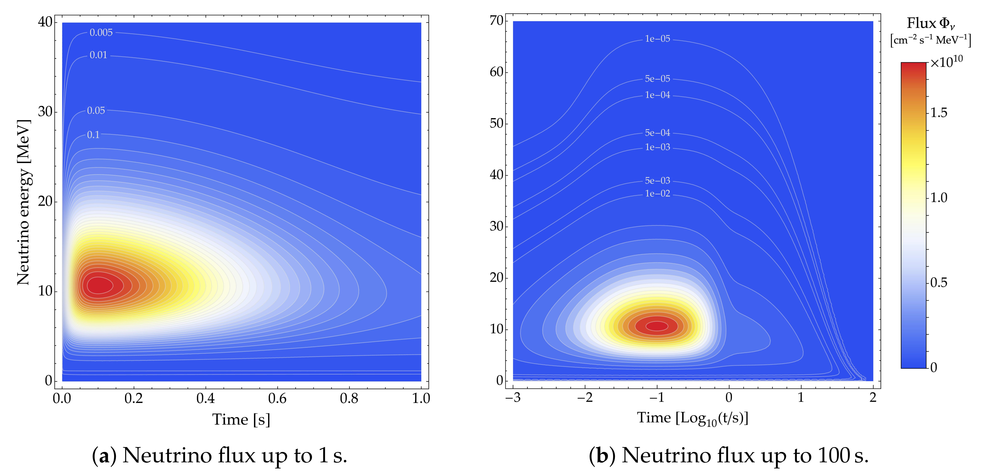
which are similar to the benchmarks (15) considered above. The total flux (1), as given by our model, is plotted in Figure 2, as a function of time and (neutrino) energy. At each time, the energy distribution resembles a thermal distribution. In Figure 2a, the initial phase is highlighted; the maximum is prominently displayed, and the order of magnitude of the flux is around ${10}^{10}{\overline{\nu }}_{\mathrm{e}}\mathrm{c}{\mathrm{m}}^{-2}{\mathrm{s}}^{-1}\mathrm{M}\mathrm{e}{\mathrm{V}}^{-1}$. Figure 2b, on the other hand, encompasses the entire time extension in logarithmic scale, up to 100 $\mathrm{s}$. It shows quite clearly the difference between accretion and cooling phases.

Figure 3 shows two important integral quantities; the luminosity (4) in Figure 3a and the fluence (6) in Figure 3b—that is, the time-integrated flux. The former has a clearly visible maximum where we have requested it to be; first, it increases linearly, then it declines, with two different time scales. The fluence turns out to be quasi thermal; the average energy we find is ${\overline{E}}_{\nu }=11.2\mathrm{M}\mathrm{e}\mathrm{V}$ (which is not very different from the best fit found by SN1987A [41,44], namely 12 $\mathrm{M}$$\mathrm{e}\mathrm{V}$). The width $\mathsf{\delta }{E}_{\nu }/{\overline{E}}_{\nu }$ is just a little bit narrower than the thermal width, which, with a Fermi–Dirac type parameterization, corresponds to a (modest) pinching parameter $\eta =0.2$.

5.2. Comparison with SN1987A

Let us now compare the model with the observations from SN1987A, which exploded in the large magellanic cloud at about $D=50\mathrm{k}\mathrm{pc}$. For illustration, we consider the 16 events seen in the detector Kamiokande-II, discussed in [42,44], which were collected in a time window of 30 $\mathrm{s}$ and which have an energy greater than $4.5$ $\mathrm{M}$$\mathrm{e}\mathrm{V}$.

The number of signal events indicated by the model (from accretion and cooling phases) are

$$N_a^{\mathrm{KII}}=6.5N_c^{\mathrm{KII}}=7.1,$$

(34)

in addition to which we expect 5.6 background events, see [42,43,44]. Thus, we have 19.2 expected events compared to the 16 observed, which is acceptable. Furthermore, the Cramér–Smirnov-von–Mises test shows that the theoretical time distribution is perfectly consistent with the observations; if the time between the first neutrino arrived and the first revealed event (which is not known) is assumed to be $t_{\mathrm{off}}=0,0.1,0.2\mathrm{s}$, the corresponding p-values are 62%, 48%, 30% respectively. Repeating the same exercise for the energy distribution, we find a p-value that indicates a similar confidence level, 51%.

For the purpose of better illustration, in Figure 4, we show the distribution functions of time and energy: we note: (1) In the case of the distribution in time, the events accumulate rapidly at first, consistently with the idea that there is a phase of emission from accretion. (2) In the case of energy distribution, there is a peculiar population of low energy events (including the last 4 events, often omitted in SN1987A data analyses) attributable to background processes, which are described as discussed in [44]. In conclusion, this model is perfectly compatible with the observations obtained on the occasion of SN1987A, even before optimizing the values of the parameters.

5.3. Predictions

To conclude, we discuss how many events that we expect from a future supernova at 10 $\mathrm{k}$$\mathrm{pc}$, supposing that the same model describes the electron antineutrino emission.

We start with Super–Kamiokande, which will be able to reconstruct the energy of the antineutrinos from the observation of the energy and direction of arrival of the events. In our model, we expect just over 5000 events, 2455 from the accretion emission and 2675 from the cooling emission (the increase w.r.t. Equation (34) is due to the larger mass of Super–Kamiokande and the closer distance of the event).

The distributions on neutrino energy and time are shown in Figure 5. The left panel shows the time of the maximum differential interaction rate, which, of course, occurs at the maximum of the luminosity (at $0.1$ $\mathrm{s}$ and, just below 20 $\mathrm{M}$$\mathrm{e}\mathrm{V}$ in our model, defined in Equation (33)); the units of measurement of the interaction rate are ${\mathrm{s}}^{-1}\mathrm{M}\mathrm{e}{\mathrm{V}}^{-1}$. The right panel instead shows in logarithmic scale both the differential rate and the time scale, in a much wider range.

In Figure 6, the interaction rate (measured in Hz) due to the signal in IceCube is given. Although this detector is not designed to measure the energy of events around tens of MeV, the counting rate in the phototubes grows so much that it becomes possible to observe the supernova signal at times around the maximum intensity, and in particular, it becomes possible to obtain evidence of the existence of an emission phase, due to accretion already after a few ms.

We emphasize that while Super–Kamiokande is equipped to distinguish the antineutrino component and to measure the energy of these events, the IceCube data analysis just described is not capable of doing either: in other words, IceCube will only measure the rate and not the energy of the events; and furthermore, their count rate will receive an additional small component from the interactions of neutrinos and antineutrinos with oxygen nuclei and electrons. This is only a small fraction of the contribution of the reaction (A2), simply because the interactions, at the energies of interest, are significantly less—see, e.g., Figure 2 of [44] and [45].

6. Variants and Possible Improvements

The above proposed model has many advantages, starting from the simplicity of its mathematical formulation, advantageous for computer analysis. It can be modified and improved in many ways. We discuss a few of them for pure purpose of illustration, stressing that the essential objective of the present work remains the one to highlight the importance of describing the first second of the emission—i.e., of the inclusion and modeling of the phase of accretion. Some other possibilities have been considered in the literature [42,43,101,102,103] using models tailored to explore SN1987A neutrinos; it is legitimate to believe that future data samples from a galactic supernova will be significantly larger, and will allow us to probe even more complex and informative models.

6.1. Variants Concerning the Cooling Component

The model discussed above considers the formation of a neutron proto-star from the earliest moments. On the other hand, it is not inevitable to believe that it is the temperature $T_c\left(t\right)$ to increase rapidly over time, as described in Equation (28), rather than the radius of the star to form rapidly. Following this line of thinking, one can alternatively consider, e.g.,

$$T_c\left(t\right)=T_0\times e^{-t/\left(4{\mathsf{\tau }}_c\right)},R_{\mathrm{ns}}\left(t\right)=R_{\mathrm{ns}0}\times \sqrt{1-e^{-t/t_0^{\prime }}},$$

(35)

see discussion in Section 4.2. On the other hand, in the first moments after collapse, the emission is completely dominated by the accretion component, and not by the cooling component, therefore this modification—which could indicate a time scale $t_0^{\prime }$ different from the one of the onset of the emission, very interesting theoretically—does not have very important practical effects, nor is it easy to see the effects in practice.

As we have repeatedly argued, in the first moments of the emission, the total luminosity of neutrinos is dominated by the accretion component. The cooling component plays a minor role in these instants and its characteristics become manifest and observable only at later times. For this reason, it is possible to adopt different parameterizations of this component, without significantly changing the position of the maximum of the luminosity, that is mainly determined by the accretion component. For instance, we can consider power laws such as

$$T_c\left(t\right)=\frac{T_0}{{(1+t/{\tau }_a)}^{\alpha /4}},R_{\mathrm{ns}}\left(t\right)=R_{\mathrm{ns}0}\times \sqrt{1-e^{-t/t_0}},$$

(36)

where $\alpha$ is a new parameter, describing the way in which the luminosity declines asymptotically.

6.2. Variants Concerning the Accretion Component

One might be interested in considering the case in which the temperature in the accretion phase changes (increases) slightly with time, before the actual moment of the explosion. In this case, one needs an extra parameter, e.g., the initial temperature $T_i$, to define

$$T_a^{\prime }\left(t\right)=0.6\times \left[T_0-(T_0-T_i)e^{-t/{\tau }_a}\right].$$

(37)

If we are interested in changing the temperature in this way, but do not want to change the brightness, we can proceed as follows. Firstly, we start from the previous model for the accretion component, defined by ${\mathsf{\Phi }}_a({\mathsf{\xi }}_{\mathrm{n}}\left(t\right),T_a\left(t\right))$ of Section 4.2, where $T_a\left(t\right)=0.6\times T_0$ is a constant; then, we replace it with the following modification:

$${\mathsf{\Phi }}_a({\mathsf{\xi }}_{\mathrm{n}}\left(t\right),T_a^{\prime }\left(t\right))\times {\left(\frac{T_a\left(t\right)}{T_a^{\prime }\left(t\right)}\right)}^{\gamma },$$

(38)

where we need to use the value of parameter $\gamma =5.5$ shown in Table 1.

6.3. Variants Concerning the Other Neutrino Flavors

It is simple to treat the flavor, proceeding in a similar manner to that often adopted to treat the time integrated flux. In fact, focusing on the cooling phase, one could reasonably assume that the spectrum of non-electronic antineutrinos (muonic, tauonic) that is involved in the study of oscillations, has the same luminosity as electronic antineutrinos, but it has a different temperature. In this way, only one parameter is added. For what concerns electron neutrinos instead, it is possible to impose the condition that the total leptonic number emitted is the one predicted by theory, constraining the emission temperature of ${\nu }_{\mathrm{e}}$. Moreover, a short initial emission component should be added. This is due to the so called “neutronization” phase, in the early stages of collapse, in which electrons combine with protons producing neutrinos. They pile up behind the shock and stream in bulk once the latter crosses the neutrinosphere. Although this emission corresponds only to a minuscule amount of events, it could be detected by future large scale detectors such as Hyper–Kamiokande or DUNE [16,103]. In this sense, the description of electron neutrinos requires considering (1) the production reaction $\mathrm{e}+\mathrm{p}\to \mathrm{n}+{\nu }_{\mathrm{e}}$ and (2) the distribution of initial electrons, i.e., a model analogous to that used in Section 3.2.2 to describe the accretion component of electron antineutrinos.

7. Discussion and Outlook

Theoretical simulations are extremely important for advancing our understanding of the supernovae, but also demanding and difficult. In spite of extensive efforts, at present, it does not appear that astrophysical models are yet able to capture fully the physics of the explosion. Undoubtedly, an observation of the neutrino signal will greatly help us make progress: it was with this consideration in mind that we conducted the present investigation.

In order to be ready when the supernova explodes, it is of some importance to have models with physically meaningful parameters that can be fitted to the observed data. We have discussed the reasons why we believe that it is necessary to include, in addition to the thermal (or quasi-thermal) components, used in most existing phenomenological studies, also a non-thermal component, which we have called the accretion component.

Such a component leads us to expect a much higher luminosity in the first second of the emission and correspondingly a very high rate of signal accumulation. It will be noted that the overall intensity of the emission in this first phase certainly plays a role for the explosion; therefore, it is reasonable to expect that direct observation will contribute significantly to fine-tune the astrophysical models of the supernova.

The specific model that we have illustrated has some aspects of practical utility, allowing, for example, to position the maximum emission, and being equipped with two distinct time scales for the decrease of luminosity during the accretion and the cooling phases. It is also equipped with an initial ramp, in which the luminosity grows. The search for the gravitational wave flux associated with gravitational collapse will benefit from the study of this initial emission phase, as already widely argued in the literature [83,84,104,105,106].

As we have illustrated, the model can be easily modified and, if necessary, improved in many ways, for example, by including a time dependence of temperature during the accretion phase, or even by changing the time dependence during the cooling phase. Several additional effects have been highlighted and discussed in the literature, and some of them may lead to observable manifestations. Careful guidance of the theory (of the simulations) would also be highly desirable to select the most plausible model parameter values and their confidence intervals.

From our point of view, the main reason for the specific parameterization proposed here is to provide a well-defined tool to discuss the existence of the accretion phase. We need to observe (anti)neutrinos from a galactic supernova in order to confidently quantify its consistency, and in particular, what its duration is and what its intensity is.

The approach we propose is complementary to that of comparing specific models calculated by astrophysicists (and lately, to see which one agrees best with the data)—see [107] for a remarkable and recent approach along these lines. In addition, the generic parameterized model, discussed in this paper, can be refined by including further specific features of interest—e.g., oscillations/fluctuations of the luminosity in the initial stage, dips and bumps expected/suggested from the theory, etc.—with the advantage of putting these phenomena in their proper context, clarifying their observability and quantifying the residual uncertainties.

References

- Murdin, P.; Murdin, L. Supernovae; Cambridge University Press: Cambridge, UK, 1978. [Google Scholar]
- Clark, D.H.; Stephenson, F.R. The Historical Supernovae; Pergamon: Oxford, UK, 1977. [Google Scholar]
- Woosley, S.E.; Weaver, T.A. The Evolution and explosion of massive stars. 2. Explosive hydrodynamics and nucleosynthesis. Astrophys. J. Suppl. 1995, 101, 181–235. [Google Scholar] [CrossRef] [Green Version]
- Thielemann, F.K.; Nomoto, K.; Hashimoto, M.A. Core-Collapse Supernovae and Their Ejecta. Astrophys. J. 1996, 460, 408. [Google Scholar] [CrossRef]
- Kobayashi, C.; Karakas, A.I.; Umeda, H. The Evolution of Isotope Ratios in the Milky Way Galaxy. Mon. Not. R. Astron. Soc. 2011, 414, 3231. [Google Scholar] [CrossRef] [Green Version]
- Nomoto, K.; Kobayashi, C.; Tominaga, N. Nucleosynthesis in Stars and the Chemical Enrichment of Galaxies. Ann. Rev. Astron. Astrophys. 2013, 51, 457–509. [Google Scholar] [CrossRef]
- Branch, D.; Wheeler, J.C. Supernova Explosions; Springer: Berlin/Heidelberg, Germany, 2017. [Google Scholar]
- Kobayashi, C.; Karakas, A.I.; Lugaro, M. The Origin of Elements from Carbon to Uranium. Astrophys. J. 2020, 900, 179. [Google Scholar] [CrossRef]
- Bethe, H.A. Supernovae. Phys. Today 1990, 43, 24–27. [Google Scholar] [CrossRef]
- Woosley, S.; Janka, T. The physics of core-collapse supernovae. Nat. Phys. 2005, 1, 147. [Google Scholar] [CrossRef]
- Janka, H.T.; Langanke, K.; Marek, A.; Martinez-Pinedo, G.; Mueller, B. Theory of Core-Collapse Supernovae. Phys. Rep. 2007, 442, 38–74. [Google Scholar] [CrossRef] [Green Version]
- Raffelt, G.G. Neutrinos and the stars. Proc. Int. Sch. Phys. Fermi 2012, 182, 61–143. [Google Scholar] [CrossRef]
- Janka, H.T. Explosion Mechanisms of Core-Collapse Supernovae. Ann. Rev. Nucl. Part. Sci. 2012, 62, 407–451. [Google Scholar] [CrossRef] [Green Version]
- Burrows, A. Colloquium: Perspectives on core-collapse supernova theory. Rev. Mod. Phys. 2013, 85, 245. [Google Scholar] [CrossRef] [Green Version]
- Foglizzo, T.; Kazeroni, R.; Guilet, J.; Masset, F.; González, M.; Krueger, B.K.; Novak, J.; Oertel, M.; Margueron, J.; Faure, J.; et al. The explosion mechanism of core-collapse supernovae: Progress in supernova theory and experiments. Publ. Astron. Soc. Aust. 2015, 32, e009. [Google Scholar] [CrossRef] [Green Version]
- Mirizzi, A.; Tamborra, I.; Janka, H.T.; Saviano, N.; Scholberg, K.; Bollig, R.; Hudepohl, L.; Chakraborty, S. Supernova Neutrinos: Production, Oscillations and Detection. La Rivista del Nuovo Cimento 2016, 39, 1–112. [Google Scholar] [CrossRef]
- Janka, H.T. Neutrino-driven Explosions. In Handbook of Supernovae; Alsabti, A., Murdin, P., Eds.; Springer: Berlin/Heidelberg, Germany, 2017. [Google Scholar] [CrossRef] [Green Version]
- Janka, H.T. Neutrino Emission from Supernovae. In Handbook of Supernovae; Alsabti, A., Murdin, P., Eds.; Springer: Berlin/Heidelberg, Germany, 2017. [Google Scholar] [CrossRef] [Green Version]
- Horiuchi, S.; Kneller, J.P. What can be learned from a future supernova neutrino detection? J. Phys. G 2018, 45, 043002. [Google Scholar] [CrossRef] [Green Version]
- Müller, B. Neutrino Emission as Diagnostics of Core-Collapse Supernovae. Ann. Rev. Nucl. Part. Sci. 2019, 69, 253–278. [Google Scholar] [CrossRef] [Green Version]
- Mezzacappa, A.; Endeve, E.; Messer, O.E.B.; Bruenn, S.W. Physical, numerical, and computational challenges of modeling neutrino transport in core-collapse supernovae. Living Rev. Relativ. 2020, 6, 4. [Google Scholar]
- Burrows, A.; Vartanyan, D. Core-Collapse Supernova Explosion Theory. Nature 2021, 589, 29–39. [Google Scholar] [CrossRef] [PubMed]
- Ott, C. The Gravitational Wave Signature of Core-Collapse Supernovae. Class. Quantum Gravity 2009, 26, 063001. [Google Scholar] [CrossRef]
- Fryer, C.L.; New, K.C.B. Gravitational waves from gravitational collapse. Living Rev. Relativ. 2011, 14, 1. [Google Scholar] [CrossRef] [Green Version]
- Ott, C.D.; Abdikamalov, E.; Mösta, P.; Haas, R.; Drasco, S.; O’Connor, E.P.; Reisswig, C.; Meakin, C.A.; Schnetter, E. General-Relativistic Simulations of Three-Dimensional Core-Collapse Supernovae. Astrophys. J. 2013, 768, 115. [Google Scholar] [CrossRef] [Green Version]
- Kuroda, T.; Takiwaki, T.; Kotake, K. Gravitational Wave Signatures from Low-mode Spiral Instabilities in Rapidly Rotating Supernova Cores. Phys. Rev. D 2014, 89, 044011. [Google Scholar] [CrossRef] [Green Version]
- Radice, D.; Morozova, V.; Burrows, A.; Vartanyan, D.; Nagakura, H. Characterizing the Gravitational Wave Signal from Core-Collapse Supernovae. Astrophys. J. Lett. 2019, 876, L9. [Google Scholar] [CrossRef] [Green Version]
- Arimoto, M.; Asada, H.; Cherry, M.L.; Fujii, M.S.; Fukazawa, Y.; Harada, A.; Hayama, K.; Hosokawa, T.; Ioka, K.; Itoh, Y.; et al. Gravitational Wave Physics and Astronomy in the Nascent Era. arXiv 2021, arXiv:2104.02445. [Google Scholar]
- Janka, H.T.; Melson, T.; Summa, A. Physics of Core-Collapse Supernovae in Three Dimensions: a Sneak Preview. Ann. Rev. Nucl. Part. Sci. 2016, 66, 341–375. [Google Scholar] [CrossRef] [Green Version]
- Müller, B. Hydrodynamics of core-collapse supernovae and their progenitors. Astrophysics 2020, 6, 3. [Google Scholar] [CrossRef]
- Hirata, K.; Kajita, T.; Koshiba, M.; Nakahata, M.; Oyama, Y.; Sato, N.; Suzuki, A.; Takita, M.; Totsuka, Y.; Kifune, T.; et al. Observation of a Neutrino Burst from the Supernova SN 1987a. Phys. Rev. Lett. 1987, 58, 1490–1493. [Google Scholar] [CrossRef] [PubMed]
- Hirata, K.; Kajita, T.; Koshiba, M.; Nakahata, M.; Oyama, Y.; Sato, N.; Suzuki, A.; Takita, M.; Totsuka, Y.; Kifune, T.; et al. Observation in the Kamiokande-II Detector of the Neutrino Burst from Supernova SN 1987a. Phys. Rev. D 1988, 38, 448–458. [Google Scholar] [CrossRef]
- Bionta, R.; Blewitt, G.; Bratton, C.B.; Casper, D.; Ciocio, A.; Claus, R.; Cortez, B.; Crouch, M.; Dye, S.T.; Errede, S.; et al. Observation of a Neutrino Burst in Coincidence with Supernova SN 1987a in the Large Magellanic Cloud. Phys. Rev. Lett. 1987, 58, 1494. [Google Scholar] [CrossRef] [Green Version]
- Bratton, C.B.; Casper, D.; Ciocio, A.; Claus, R.; Crouch, M.; Dye, S.T.; Errede, S.; Gajewski, W.; Goldhaber, M.; Haines, T.J.; et al. Angular Distribution of Events From Sn1987a. Phys. Rev. D 1988, 37, 3361. [Google Scholar] [CrossRef]
- Alekseev, E.; Alekseeva, L.; Krivosheina, I.; Volchenko, V. Detection of the Neutrino Signal From SN1987A in the LMC Using the Inr Baksan Underground Scintillation Telescope. Phys. Lett. B 1988, 205, 209–214. [Google Scholar] [CrossRef]
- Colgate, S.A.; Johnson, M.H. Hydrodynamic Origin of Cosmic Rays. Phys. Rev. Lett. 1960, 5, 235–238. [Google Scholar] [CrossRef]
- Colgate, S.A.; White, R.H. The Hydrodynamic Behavior of Supernovae Explosions. Astrophys. J. 1966, 143, 626. [Google Scholar] [CrossRef]
- Wilson, J.R. A Numerical Study of Gravitational Stellar Collapse. Astrophys. J. 1971, 163, 209. [Google Scholar] [CrossRef]
- Nadyozhin, D. The neutrino radiation for the hot neutron star formation and the envelope outburst problem. Astrophys. Space Sci. 1978, 53, 131–153. [Google Scholar] [CrossRef]
- Bethe, H.A.; Wilson, J.R. Revival of a stalled supernova shock by neutrino heating. Astrophys. J. 1985, 295, 14–23. [Google Scholar] [CrossRef]
- Bahcall, J.N. Neutrino Astrophysics; Cambridge University Press: Cambridge, UK, 1989. [Google Scholar]
- Loredo, T.J.; Lamb, D.Q. Bayesian analysis of neutrinos observed from supernova SN-1987A. Phys. Rev. D 2002, 65, 063002. [Google Scholar] [CrossRef] [Green Version]
- Pagliaroli, G.; Vissani, F.; Costantini, M.L.; Ianni, A. Improved analysis of SN1987A antineutrino events. Astropart. Phys. 2009, 31, 163–176. [Google Scholar] [CrossRef] [Green Version]
- Vissani, F. Comparative analysis of SN1987A antineutrino fluence. J. Phys. G 2015, 42, 013001. [Google Scholar] [CrossRef]
- Scholberg, K. Supernova Neutrino Detection. Ann. Rev. Nucl. Part. Sci. 2012, 62, 81–103. [Google Scholar] [CrossRef] [Green Version]
- Rozwadowska, K.; Vissani, F.; Cappellaro, E. On the rate of core collapse supernovae in the milky way. New Astron. 2021, 83, 101498. [Google Scholar] [CrossRef]
- Fukuda, S.; Fukuda, Y.; Hayakawa, T.; Ichihara, E.; Ishitsuka, M.; Itow, Y.; Kajita, T.; Kameda, J.; Kaneyuki, K.; Kasuga, S.; et al. The Super-Kamiokande detector. Nucl. Instrum. Methods A 2003, 501, 418–462. [Google Scholar] [CrossRef]
- Beacom, J.F.; Vagins, M.R. GADZOOKS! Anti-neutrino spectroscopy with large water Cherenkov detectors. Phys. Rev. Lett. 2004, 93, 171101. [Google Scholar] [CrossRef] [Green Version]
- Simpson, C.; Abe, K.; Bronner, C.; Hayato, Y.; Ikeda, M.; Ito, H.; Iyogi, K.; Kameda, J.; Kataoka, Y.; Kato, Y.; et al. Sensitivity of Super-Kamiokande with Gadolinium to Low Energy Anti-neutrinos from Pre-supernova Emission. Astrophys. J. 2019, 885, 133. [Google Scholar] [CrossRef] [Green Version]
- Abbasi, R.; Abdou, Y.; Abu-Zayyad, T.; Ackermann, M.; Adams, J.; Aguilar, J.A.; Ahlers, M.; Allen, M.M.; Altmann, D.; Andeen, K.; et al. IceCube Sensitivity for Low-Energy Neutrinos from Nearby Supernovae. Astron. Astrophys. 2011, 535, A109, Erratum in 2014, 563, C1. [Google Scholar] [CrossRef] [Green Version]
- Dadykin, V.L.; Zatsepin, G.T.; Korchagin, V.B.; Korchagin, P.V.; Mal’Gin, A.S.; Ryazhskaya, O.G.; Ryasny, V.G.; Talochkin, V.P.; Khal’Chukov, F.F.; Yakushev, V.F.; et al. Detection of a Rare Event on 23 February 1987 by the Neutrino Radiation Detector under Mont Blanc. JETP Lett. 1987, 45, 593–595. [Google Scholar]
- Ryazhskaya, O.G. Problems of Neutrino Radiation from SN 1987A: 30 Years Later. Phys. At. Nucl. 2018, 81, 113–119. [Google Scholar] [CrossRef]
- Galeotti, P.; Pizzella, G. New analysis for the correlation between gravitational wave and neutrino detectors during SN1987A. Eur. Phys. J. C 2016, 76, 426. [Google Scholar] [CrossRef] [Green Version]
- Vissani, F.; Costantini, M.L.; Fulgione, W.; Ianni, A.; Pagliaroli, G. What is the issue with SN1987A neutrinos? Ital. Phys. Soc. Proc. 2011, 103, 611–619. [Google Scholar]
- Orlando, S. Linking Core-Collapse Supernova Explosions to Supernova Remnants through 3D MHD Modeling: The Case of SN 1987A. Talk at the Workshop “Core-Collapse Supernovae in the Multi-Messenger Era”, L’Aquila, Italy, 2–3 July 2018. [Google Scholar]
- Ono, M.; Nagataki, S.; Ferrand, G.; Takahashi, K.; Umeda, H.; Yoshida, T.; Orlando, S.; Miceli, M. Matter Mixing in Aspherical Core-collapse Supernovae: Three-dimensional Simulations with Single Star and Binary Merger Progenitor Models for SN 1987A. Astrophys. J. 2020, 888, 111. [Google Scholar] [CrossRef]
- Page, D.; Beznogov, M.V.; Garibay, I.; Lattimer, J.M.; Prakash, M.; Janka, H.T. NS 1987A in SN 1987A. Astrophys. J. 2020, 898, 125. [Google Scholar] [CrossRef]
- Costantini, M.L.; Ianni, A.; Vissani, F. SN1987A and the properties of neutrino burst. Phys. Rev. D 2004, 70, 043006. [Google Scholar] [CrossRef] [Green Version]
- Pantaleone, J.T. Neutrino oscillations at high densities. Phys. Lett. B 1992, 287, 128–132. [Google Scholar] [CrossRef]
- Samuel, S. Neutrino oscillations in dense neutrino gases. Phys. Rev. D 1993, 48, 1462–1477. [Google Scholar] [CrossRef]
- Sigl, G.; Raffelt, G. General kinetic description of relativistic mixed neutrinos. Nucl. Phys. B 1993, 406, 423–451. [Google Scholar] [CrossRef]
- Dighe, A.S.; Smirnov, A.Y. Identifying the neutrino mass spectrum from the neutrino burst from a supernova. Phys. Rev. D 2000, 62, 033007. [Google Scholar] [CrossRef] [Green Version]
- Duan, H.; Kneller, J.P. Neutrino flavour transformation in supernovae. J. Phys. G 2009, 36, 113201. [Google Scholar] [CrossRef] [Green Version]
- Duan, H.; Fuller, G.M.; Qian, Y.Z. Collective Neutrino Oscillations. Ann. Rev. Nucl. Part. Sci. 2010, 60, 569–594. [Google Scholar] [CrossRef] [Green Version]
- Volpe, C. Neutrino Quantum Kinetic Equations. Int. J. Mod. Phys. E 2015, 24, 1541009. [Google Scholar] [CrossRef] [Green Version]
- Glas, R.; Janka, H.T.; Capozzi, F.; Sen, M.; Dasgupta, B.; Mirizzi, A.; Sigl, G. Fast Neutrino Flavor Instability in the Neutron-star Convection Layer of Three-dimensional Supernova Models. Phys. Rev. D 2020, 101, 063001. [Google Scholar] [CrossRef] [Green Version]
- Tamborra, I.; Shalgar, S. New Developments in Flavor Evolution of a Dense Neutrino Gas Annual. Rev. Nucl. Part. Sci. 2020, 71, 165–188. [Google Scholar] [CrossRef]
- Wolfenstein, L. Neutrino Oscillations in Matter. Phys. Rev. D 1978, 17, 2369–2374. [Google Scholar] [CrossRef]
- Mikheyev, S.P.; Smirnov, A.Y. Resonance Amplification of Oscillations in Matter and Spectroscopy of Solar Neutrinos. Sov. J. Nucl. Phys. 1985, 42, 913–917. [Google Scholar]
- Bahcall, J.N.; Krastev, P.I.; Smirnov, A.Y. Is large mixing angle MSW the solution of the solar neutrino problems? Phys. Rev. D 1999, 60, 093001. [Google Scholar] [CrossRef] [Green Version]
- Minakata, H.; Nunokawa, H. Inverted hierarchy of neutrino masses disfavored by supernova 1987A. Phys. Lett. B 2001, 504, 301–308. [Google Scholar] [CrossRef] [Green Version]
- Barger, V.; Marfatia, D.; Wood, B.P. Supernova 1987A did not test the neutrino mass hierarchy. Phys. Lett. B 2002, 532, 19–28. [Google Scholar] [CrossRef] [Green Version]
- Minakata, H.; Nunokawa, H.; Tomas, R.; Valle, J.W.F. Probing supernova physics with neutrino oscillations. Phys. Lett. B 2002, 542, 239–244. [Google Scholar] [CrossRef] [Green Version]
- Minakata, H.; Nunokawa, H.; Tomas, R.; Valle, J.W.F. Parameter Degeneracy in Flavor-Dependent Reconstruction of Supernova Neutrino Fluxes. JCAP 2008, 12, 006. [Google Scholar] [CrossRef]
- Nagakura, H.; Hotokezaka, K. Non-thermal neutrinos created by shock acceleration in successful and failed core-collapse supernova. Mon. Not. R. Astron. Soc. 2021, 502, 89–107. [Google Scholar] [CrossRef]
- Mirizzi, A.; Raffelt, G.G. New analysis of the sn 1987a neutrinos with a flexible spectral shape. Phys. Rev. D 2005, 72, 063001. [Google Scholar] [CrossRef] [Green Version]
- Lunardini, C. The diffuse supernova neutrino flux, supernova rate and sn1987a. Astropart. Phys. 2006, 26, 190–201. [Google Scholar] [CrossRef] [Green Version]
- Buras, R.; Rampp, M.; Janka, H.T.; Kifonidis, K. Two-dimensional hydrodynamic core-collapse supernova simulations with spectral neutrino transport. 1. Numerical method and results for a 15 solar mass star. Astron. Astrophys. 2006, 447, 1049–1092. [Google Scholar] [CrossRef] [Green Version]
- Vissani, F.; Pagliaroli, G. How much can we learn from SN1987A events? Or: An analysis with a two-Component model for the antineutrino signal. In Proceedings of the 4th International Workshop on Neutrino Oscillations in Venice: Ten Years after the Neutrino Oscillations, Venice, Italy, 15–18 April 2008. [Google Scholar]
- Smarr, L.; Wilson, J.R.; Barton, R.T.; Bowers, R.L. Rayleigh-taylor overturn in supernova core collapse. Astrophys. J. 1981, 246, 515–525. [Google Scholar] [CrossRef]
- Fantini, G.; Gallo Rosso, A.; Vissani, F.; Zema, V. Introduction to the Formalism of Neutrino Oscillations. Adv. Ser. Dir. High Energy Phys. 2018, 28, 37–119. [Google Scholar] [CrossRef]
- Capozzi, F.; Di Valentino, E.; Lisi, E.; Marrone, A.; Melchiorri, A.; Palazzo, A. The unfinished fabric of the three neutrino paradigm. arXiv 2021, arXiv:2107.00532. [Google Scholar]
- Pagliaroli, G.; Vissani, F.; Coccia, E.; Fulgione, W. Neutrinos from Supernovae as a Trigger for Gravitational Wave Search. Phys. Rev. Lett. 2009, 103, 031102. [Google Scholar] [CrossRef] [Green Version]
- Halzen, F.; Raffelt, G.G. Reconstructing the supernova bounce time with neutrinos in IceCube. Phys. Rev. D 2009, 80, 087301. [Google Scholar] [CrossRef] [Green Version]
- Iida, T. Search for Supernova Relic Neutrino at Super-Kamiokande. Ph.D. Thesis, The University of Tokyo, Tokyo, Japan, 2010. [Google Scholar]
- Kowarik, T.; Griesel, T.; Piegsa, A. Supernova Search with the AMANDA / IceCube Detectors. In Proceedings of the 31st ICRC, Lodz, Poland, 7–15 July 2009. [Google Scholar]
- An, F.; An, G.; An, Q.; Antonelli, V.; Baussan, E.; Beacom, J.; Bezrukov, L.; Blyth, S.; Brugnera, R.; Avanzini, M.B.; et al. Neutrino Physics with JUNO. J. Phys. G 2016, 43, 030401. [Google Scholar] [CrossRef]
- Abi, B.; Acciarri, R.; Acero, M.A.; Adamov, G.; Adams, D.; Adinolfi, M.; Ahmad, Z.; Ahmed, J.; Alion, T.; Monsalve, S.A.; et al. Supernova neutrino burst detection with the Deep Underground Neutrino Experiment. Eur. Phys. J. C 2021, 81, 423. [Google Scholar] [CrossRef]
- Aiello, S.; Albert, A.; Garre, S.A.; Aly, Z.; Ambrosone, A.; Ameli, F.; Andre, M.; Androulakis, G.; Anghinolfi, M.; Anguita, M.; et al. The KM3NeT potential for the next core-collapse supernova observation with neutrinos. Eur. Phys. J. C 2021, 81, 445. [Google Scholar] [CrossRef]
- Monzani, M.E. Supernova neutrino detection in Borexino. Il Nuovo Cimento C 2006, 29, 269–280. [Google Scholar] [CrossRef]
- Lang, R.F.; McCabe, C.; Reichard, S.; Selvi, M.; Tamborra, I. Supernova neutrino physics with xenon dark matter detectors: A timely perspective. Phys. Rev. D 2016, 94, 103009. [Google Scholar] [CrossRef] [Green Version]
- Gallo Rosso, A. Supernova neutrino fluxes in HALO-1kT, Super-Kamiokande, and JUNO. JCAP 2021, 06, 046. [Google Scholar] [CrossRef]
- Kistler, M.D.; Yuksel, H.; Ando, S.; Beacom, J.F.; Suzuki, Y. Core-Collapse Astrophysics with a Five-Megaton Neutrino Detector. Phys. Rev. D 2011, 83, 123008. [Google Scholar] [CrossRef] [Green Version]
- Burrows, A.; Klein, D.; Gandhi, R. The Future of supernova neutrino detection. Phys. Rev. D 1992, 45, 3361–3385. [Google Scholar] [CrossRef] [PubMed]
- Skadhauge, S.; Zukanovich Funchal, R. Determining neutrino and supernova parameters with a galactic supernova. JCAP 2007, 04, 014. [Google Scholar] [CrossRef] [Green Version]
- Keehn, J.G.; Lunardini, C. Neutrinos from failed supernovae at future water and liquid argon detectors. Phys. Rev. D 2012, 85, 043011. [Google Scholar] [CrossRef] [Green Version]
- Lujan-Peschard, C.; Pagliaroli, G.; Vissani, F. Spectrum of Supernova Neutrinos in Ultra-pure Scintillators. JCAP 2014, 07, 051. [Google Scholar] [CrossRef] [Green Version]
- Gallo Rosso, A.; Vissani, F.; Volpe, M.C. What can we learn on supernova neutrino spectra with water Cherenkov detectors? JCAP 2018, 4, 040. [Google Scholar] [CrossRef] [Green Version]
- Nagakura, H. Retrieval of energy spectra for all flavours of neutrinos from core-collapse supernova with multiple detectors. Mon. Not. R. Astron. Soc. 2020, 500, 319–332. [Google Scholar] [CrossRef]
- Al Kharusi, S.; BenZvi, S.Y.; Bobowski, J.S.; Bonivento, W.; Brdar, V.; Brunner, T.; Caden, E.; Clark, M.; Coleiro, A.; Colomer-Molla, M.; et al. SNEWS 2.0: A next-generation supernova early warning system for multi-messenger astronomy. New J. Phys. 2021, 23, 031201. [Google Scholar] [CrossRef]
- Abbott, L.F.; De Rujula, A.; Walker, T.P. Constraints on the Neutrino Mass From the Supernova Data: A Systematic Analysis. Nucl. Phys. B 1988, 299, 734–756. [Google Scholar] [CrossRef]
- Nardi, E.; Zuluaga, J.I. Exploring the sub-eV neutrino mass range with supernova neutrinos. Phys. Rev. D 2004, 69, 103002. [Google Scholar] [CrossRef] [Green Version]
- Pagliaroli, G.; Rossi-Torres, F.; Vissani, F. Neutrino mass bound in the standard scenario for supernova electronic antineutrino emission. Astropart. Phys. 2010, 33, 287–291. [Google Scholar] [CrossRef] [Green Version]
- Leonor, I.; Cadonati, L.; Coccia, E.; D’Antonio, S.; Di Credico, A.; Fafone, V.; Frey, R.; Fulgione, W.; Katsavounidis, E.; Ott, C.D.; et al. Searching for prompt signatures of nearby core-collapse supernovae by a joint analysis of neutrino and gravitational-wave data. Class. Quantum Gravity 2010, 27, 084019. [Google Scholar] [CrossRef] [Green Version]
- Abbott, B.P.; Abbott, R.; Abbott, T.D.; Abernathy, M.R.; Acernese, F.; Ackley, K.; Adams, C.; Adams, T.; Addesso, P.; Adhikari, R.X.; et al. A First Targeted Search for Gravitational-Wave Bursts from Core-Collapse Supernovae in Data of First-Generation Laser Interferometer Detectors. Phys. Rev. D 2016, 94, 102001. [Google Scholar] [CrossRef] [Green Version]
- Abdikamalov, E.; Pagliaroli, G.; Radice, D. Gravitational Waves from Core-Collapse Supernovae. arXiv 2020, arXiv:2010.04356. [Google Scholar]
- Abe, K.; Adrich, P.; Aihara, H.; Akutsu, R.; Alekseev, I.; Ali, A.; Ameli, F.; Anghel, I.; Anthony, L.H.V.; Antonova, M.; et al. Supernova Model Discrimination with Hyper-Kamiokande. Astrophys. J. 2021, 916, 15. [Google Scholar] [CrossRef]
- Strumia, A.; Vissani, F. Precise quasielastic neutrino/nucleon cross-section. Phys. Lett. B 2003, 564, 42–54. [Google Scholar] [CrossRef] [Green Version]