Spectral Norm Regularization for Blind Image Deblurring

Abstract

Blind image deblurring is a well-known ill-posed inverse problem in the computer vision field. To make the problem well-posed, this paper puts forward a plain but effective regularization method, namely spectral norm regularization (SN), which can be regarded as the symmetrical form of the spectral norm. This work is inspired by the observation that the SN value increases after the image is blurred. Based on this observation, a blind deblurring algorithm (BDA-SN) is designed. BDA-SN builds a deblurring estimator for the image degradation process by investigating the inherent properties of SN and an image gradient. Compared with previous image regularization methods, SN shows more vital abilities to differentiate clear and degraded images. Therefore, the SN of an image can effectively help image deblurring in various scenes, such as text, face, natural, and saturated images. Qualitative and quantitative experimental evaluations demonstrate that BDA-SN can achieve favorable performances on actual and simulated images, with the average PSNR reaching 31.41, especially on the benchmark dataset of Levin et al.

1. Introduction

Blind deblurring, or blind deconvolution, has received considerable attention in the field of image processing and computer vision. The most typical example is the motion blur caused by a mobile phone shaking when taking pictures. In addition, the movement of the target object, bad weather, poor focus, insufficient light, etc., are all causes of image degradation. The blur kernel is assumed to be space-invariant. The blurred image $g(x,y)$ obtained is expressed as the convolution of the kernel $h(x,y)$ and the clear image $o(x,y)$. The kernel is also referred to the point spread function (PSF) [1], which leads to image degradation. The blurring process can be modeled as follows [2]:

$$g(x,y)=o(x,y)\ast h(x,y)+n(x,y)$$

(1)

where “*” stands for the convolution operator; $o(x,y)$ and $g(x,y)$ represent clear images and blurred versions, respectively; $h(x,y)$ denotes the kernel representing degradation induced in the spatial domain; and $n(x,y)$ stands for the inevitable noise.

In blind deblurring, only the blurred version $g(x,y)$ is known; thus, we have to calculate the kernel $h(x,y)$ and the clear image $o(x,y)$ through the obtained blurred image $g(x,y)$, simultaneously. Obviously, this problem is highly ill-posed. In theory, infinite solution pairs $o(x,y)$ and $h(x,y)$ correspond to $g(x,y)$. The delta kernel and blurred images are the most typical solutions. To alleviate this inherently ill-posed problem, image priors and appropriate regularization are employed [3]. Various statistical priors are incorporated into the associated variational model to tackle this challenging inverse problem. The statistical priors about images mainly include image gradient sparse priors [4,5,6], L0 regularized priors [7,8,9], low-rank priors [10,11], dark channel priors [9], deep discrimination priors [12], extreme channel priors [13], and patch-based priors [14,15]. Moreover, many specially designed priors [16,17] are exploited. The maximum a posterior (MAP) framework [18] is used by most of the above algorithms. The solution space is constrained, and the possibility of the algorithm producing trivial solutions is reduced. Most of the priors mentioned above are about image gradient priors. The information about the image itself needs to be better utilized. Therefore, it makes sense to establish a prior that is more relevant to the image domain.

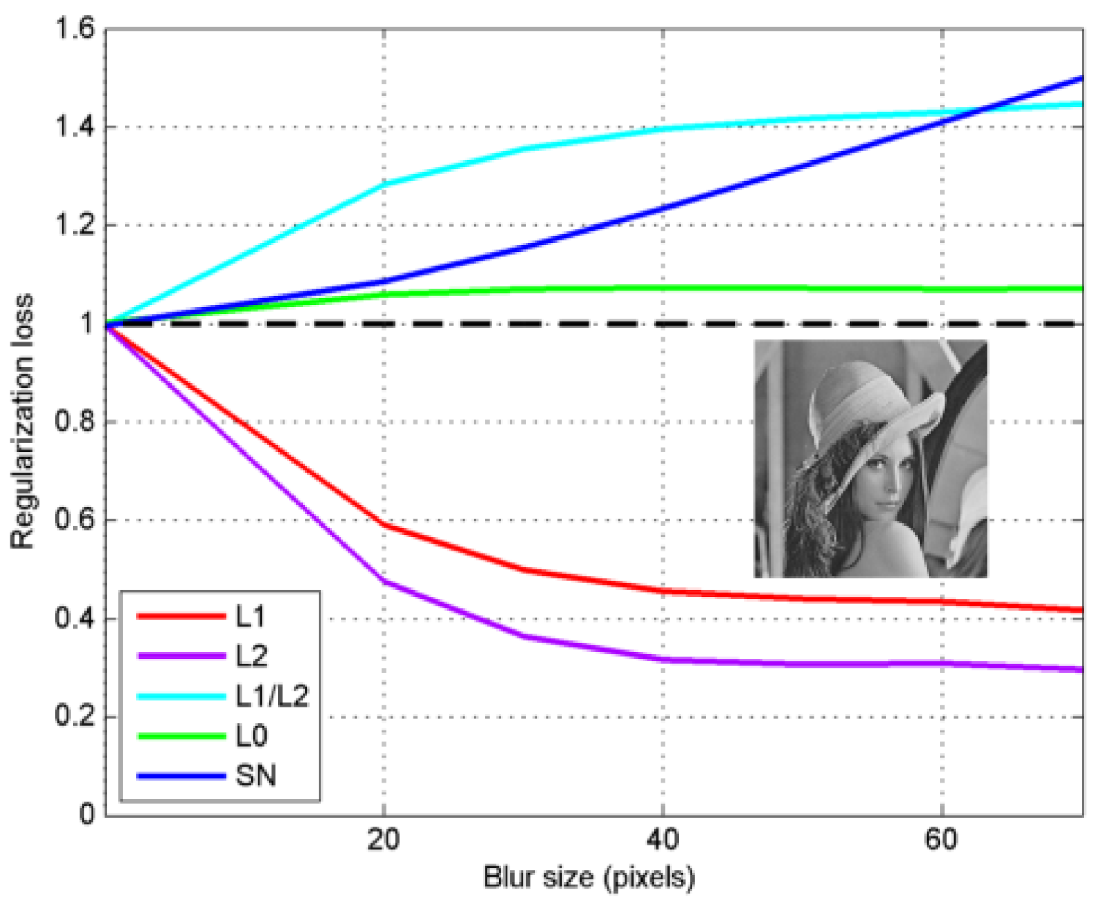
This paper proposes a prior that is directly related to the image, that is, spectral norm regularization (SN). Its form is $\frac{{\parallel o\parallel }_1}{\sigma \left(o\right)}$, where $\sigma \left(o\right)$ is the spectral norm of the image. SN and other regularizations will be compared in detail in Section 3. As shown in Figure 1, the SN value is positively correlated with the degree of image degradation. Based on this discovery, a blind deblurring algorithm using SN is proposed.

Figure 1. Regularization losses vary with blur size. (The losses are given by $F(\nabla x(o\ast h\left)\right)+F(\nabla y(o\ast h\left)\right)$, where $F\left(x\right)$ is the regular function, and $\nabla x$ and $\nabla y$ represent discrete gradient filters. The size of h ranges from 1 to 70 pixels).

The core contributions are as follows:

(1)

This paper proposes a prior, named spectral norm regularization (SN). Different from existing image gradient priors, SN is a prior about the image domain. The SN value becomes larger when the image becomes blurred. As a result, SN can easily distinguish between degraded and clear images.

(2)

This paper proposed a novel algorithm to utilize the property of SN, named BDA-SN. BDA-SN can use not only the information brought by the image gradient domain but also the information brought by the image domain. Therefore, BDA-SN can better deal with blind deblurring.

(3)

Extensive experiments demonstrate that BDA-SN can achieve good performances on actual and simulated images. Qualitative and quantitative evaluations indicate that BDA-SN is superior to other state-of-the-art methods.

2. Related Work

In the past ten years, deblurring algorithms for single images have made great progress. There are two main methods. One is through statistical priors of natural images, and the other is via deep learning.

Scholars developed various statistical priors on image distribution in order to efficiently calculate the kernel. After investigating the variational Bayesian inference, Fergus et al. [4] introduced a mixture of Gaussian models to fit the gradient distribution. To better fit the gradient of the heavy-tailed distribution, a piecewise function was adopted by Shan et al. [6]. Levin et al. [5] found that the maximum a posterior (MAP) method often produces trivial solutions and introduced an effective maximum margin strategy. Krishnan et al. [19] exploited the L1/L2 function to restrict the sparsity of the gradient. Xu and Jia [7] found a more sparse prior; that is, the generalized L0 regularization prior, which not only improves the restoration quality but also speeds up algorithm efficiency. For text images, Pan et al. [9] investigated the sparsity of image pixel intensity. Jin [20] designed a blind deblurring strategy with high accuracy and robustness to noise. Bai et al. [21] exploited the re-weighted total variation of the graph (RGTV) prior that derives the blur kernel efficiently. L0 regularization is widely used in image restoration and has achieved excellent results. Li et al. [12] utilized L0 regularization to constrain the blur kernel. In this paper, the L0 regularization prior is also adopted in the proposed blind deblurring model.

In the MAP framework, the estimation of the kernel benefits from sharp edges. Therefore, algorithms that use explicit edge extraction [22,23] have received widespread attention. Using a gradient threshold to retrieve strong edges is the main edge extraction method at present. The explicit edge extraction method has obvious defects; In other words, some images have no obvious edges to retrieve [24]. This method not only leads to over-sharpening of the image but also to the amplification of noise.

The gradient prior and the intensity prior are mainly applied to a single pixel or adjacent pixels, ignoring the relationship in a larger range. In order to better reflect the relationship within the image, many patch-based algorithms have been exploited. Inspired by the statistical priors of natural images, Sun et al. [25] adopted two priors based on patch edges. Ren et al. [10] developed a blind deblurring method combining self-similar characteristics of image patches with low-rank prior. By combining low ranking constraint and salient edge selection, Dong et al. [11] developed an algorithm that can protect edges while removing blur. Hsieh et al. [26] proposed a strongly imposed zero patch minimum constraint for blind image deblurring. These patch-based methods require a patch search, so more running time is required. Tang et al. [15] used sparse representation with external patch priors for image deblurring. Pan et al. [9] analyzed the changes in the dark channel after the image was blurred and introduced a blind deblurring algorithm via a dark channel prior, which achieves good performance in different scenes. Yan et al. [13] combined a bright channel with a dark channel and utilized the extreme channel for image restoration. Although Pan et al. [9] and Yan et al. [13] have achieved good results, they obviously encountered certain limitations. Sometimes, the image did not have obvious dark pixels and bright pixels and the blur kernel could not be effectively estimated. Inspired by the dark channel prior, Wen and Ying [27] proposed sparse regularization using the local minimum pixel, which improves the speed of the algorithm. At the same time, Chen et al. [16] proposed the local maximum gradient prior (LMG) for blind deblurring, and LMG has reached satisfactory performance in a variety of scenes. Xu et al. [24] simplified LMG and derived the patch maximum gradient prior (PMG), which lowered the cost of calculation. Algorithms based on image priors are difficult to use to restore images of specific scenes [28]. Therefore, some algorithms for special scenes have been exploited, such as text [9], saturated [29], and face images [29]. However, these specific algorithms often lack generalization and have poor restoration effects on other special scene images. Table 1 summarizes the strengths and weaknesses of BDA-SN and previous methods.

Table 1. Comparison of BDA-SN with previous methods.

Methods	Strengths	Weaknesses
Krishnan et al. [19]	Uses L1/L2 regularization to constrain the sparsity of the image gradient. The algorithm is efficient.	L1/L2 is non-convex. The restored image has strong artifacts.
Xu et al. [7]	Uses generalized L0 regularization, which improves the restoration quality.	L0 is non-convex. The deblurring effect is poor.
Pan et al. [9]	Uses dark channel, which can easily distinguish between clear and degraded images.	The method performs poorly on images without obvious dark pixels.
Yan et al. [13]	Combines both the dark channel and the bright channel information. No complicated processing techniques and edge selection steps are required.	The method performs poorly on images without obvious dark or bright pixels.
Jin et al. [20]	Uses constraint ${\parallel k\parallel }_p{\parallel \nabla x\parallel }_2$ to to fix the scale ambiguity, and proposes a blind deblurring strategy with high accuracy and robustness to noise.	High computational cost.
Bai et al. [21]	Uses the re-weighted total variation of the graph (RGTV) prior that derives the blur kernel efficiently.	This is a non-convex and non-differentiable optimization problem that requires additional strategies.
Wen et al. [27]	Uses the patch-wise minimal pixels (PMP) prior, which is very effective in discriminating between clear and blurred images. The algorithm is efficient.	This method performs poorly on images with large pixel values.
BDA-SN	Uses the prior SN of the image domain, which has a strong ability to distinguish clear and blurred images.	High computational cost.

In recent years, deep neural networks have developed rapidly, and data-driven methods have made great progress. Nah and Hyun [30] adopted a convolutional neural network (CNN) with multiple scales, which does not need to make any assumptions about the kernel and recovers images with an end-and-end method. Su et al. [31] used a deep learning method to deblur the video with trained CNN. Kupyn et al. [32] exploited an end-and-end learning approach, which utilizes conditional generative adversarial networks (GAN) to remove motion blur. Zhao et al. [33] developed an improved deep multi-patch hierarchical network that has a powerful and complex representation for dynamic scene deblurring. Almansour et al. [34] investigated the impact of a super-resolution reconstruction technique using deep leaning on abdominal magnetic resonance imaging. Li et al. [35] developed a single-image high-fidelity blind deblurring method that embedded a CNN prior before MAP. Although these data-driven ways reached excellent results, the effects severely depend on the similarity of the test dataset and the training dataset. Therefore, the generalization of data-driven strategies is poor, and the computational cost is huge.

Having reviewed the progress of image restoration of the last decade in this section, the rest of this work is as follows. In Section 3, this paper introduces a blind deblurring algorithm using spectral norm regularization (BDA-SN) in detail. In Section 4, this paper presents some experimental results for performance evaluation, which are compared with the latest methods. Section 5 provides an analysis and discussion about the effectiveness of BDA-SN. Section 6 gives a summary of this paper.

3. Methods

3.1. Spectral Normalization

This section first describes spectral norm regularization (SN) and then its advantage in blind image deblurring. The spectral norm of a matrix A is defined by

$$\sigma \left(A\right)=\sqrt{{\lambda }_{max}}={\sigma }_1$$

(2)

where ${\lambda }_{max}$ is the maximum eigenvalue of $A^{H}A$, ${\sigma }_1$ is the maximum singular value of A, and $A^H$ is the transposed-conjugate matrix of A. For an image $o(x,y)$, the spectral norm regularization (SN) is defined by

$$SN=\frac{{\parallel o\parallel }_1}{\sigma \left(o\right)}$$

(3)

The spectral norm regularization (SN) is based on an observation that, in an image, the SN value becomes larger after the blurring process. To better illustrate this property, an example of different regularization losses is shown in Figure 1, which reveals the degradation caused by atmospheric turbulence. Blur kernels are simulated by a random phase screen [36].

As shown in Figure 1, L1 and L2 regularization decrease as the degree of blur becomes larger. L1 and L2 regularization are more friendly to blurred images, so they are not proper regularizations [5]. Krishnan et al. [19] proposed L1/L2 regularization, which is more friendly to clear images than blurred images. Inspired by L1/L2 regularization, this paper adopts SN, which shows more vital abilities to differentiate clear and degraded images. Next, this paper gives a detailed comparison between SN and other regularization.

3.2. Comparison with Other Regularizations

Different from other gradient domain regularizations, this paper presents an image domain regularization. SN can better describe the image domain rather than the gradient domain. BDA-SN combines the regularization method of gradient domain and image domain. BDA-SN is an enhanced sparse method. Therefore, BDA-SN can better distinguish between clear images and blurred images.

Comparison with L2 regularization: L2 regularization is a famous blind image deblurring regularization. The L2 regularization can make the model meet the Lipschitz continuity better, thus reducing the sensitivity of the model to input perturbation and enhancing the generalization performance of the model. Therefore, it can be considered that the L2 regularization reduces the sum of squared singular values [37]. Although the model using L2 regularization is insensitive to perturbation and the model is valid, L2 regularization loses important information about the image, because the image acts as an operator contracting in all directions under the constraint of L2 regularization. In contrast, spectral norm regularization focuses only on the first singular value, so the image matrix does not significantly shrink in the direction orthogonal to the first right singular vector. Obviously, SN can retain more information of the image itself. In other words, BDA-SN can achieve greater complexity and can better describe image information.

Comparison with L1/L2 regularization: SN is similar to L1/L2 regularization in form, but they are two utterly different regularization methods. As mentioned above, SN is applied to the image domain, while L1/L2 regularization is applied to the gradient domain. At the same time, BDA-SN uses the spectral norm instead of the L2 norm.

Comparison with spectral norm regularization: Nevertheless, here, we emphasize the difference between spectral norm regularization and spectral norm regularization. Spectral norm regularization, L1 regularization, and L2 regularization add explicit regularization terms to the loss function. Spectral norm regularization is used to punish the spectral norm. To some extent, spectral norm regularization is a normalized version of spectral norm regularization. Spectral norm regularization attempts to set the spectral norm to a specified interval by constraining the spectral norm of the image after each iteration [38]. Therefore, BDA-SN can deal with images in a variety of different scenarios well. The use of spectral norm regularization makes BDA-SN more robust.

3.3. BDA-SN

Based on the property that SN can easily differentiate degraded and clear images, a novel deblurring algorithm is devised by adopting SN, i.e., BDA-SN. The least-squares algorithm is almost insensitive to whether noise is Gaussian or Poissonian [39]. For Poissonian noise, there is no significant difference between the effects of RLA and ISRA, while for Gaussian noise, ISRA can achieve better results than RLA [40]. Here, due to the robustness of the Gaussian noise assumption, the likelihood probability function [41] can be modeled as

$$P\left(g\right|o,h)=\prod _{x,y}\frac{1}{\sqrt{2\pi }\sigma }exp(-\frac{{[g(x,y)-h(x,y)\ast o(x,y)]}^2}{2{\sigma }^2})$$

(4)

where ${\sigma }^2$ denotes the variance of the noise, $g(x,y)$ represents the degraded image, $o(x,y)$ denotes the clear image, and $h(x,y)$ represents the kernel. The corresponding log-likelihood probability function multiplied by ${\sigma }^2$ is

$${\sigma }^{2}log\left[P\left(g\right|o,h)\right]=\sum _{x,y}{\sigma }^{2}log\left[\frac{1}{\sqrt{2\pi }\sigma }\right]-\sum _{x,y}\frac{{[g(x,y)-h(x,y)\ast o(x,y)]}^2}{2}$$

(5)

$$\begin{array}{cc}\hfill J(o,h)& =-{\sigma }^{2}log\left[P\left(g\right|o,h)\right]\hfill \\ & =\sum _{x,y}\frac{{[g(x,y)-h(x,y)\ast o(x,y)]}^2}{2}+C\hfill \\ \hfill & ={\parallel g(x,y)-h(x,y)\ast o(x,y)\parallel }^2+C\hfill \end{array}$$

(6)

where C denotes a constant and $J(o,h)$ represents the loss function. Obviously, the problem is heavily ill-posed because numerous different solution pairs $(o,h)$ give rise to the same $g(x,y)$ [9]. In order to make blind deblurring well-posed, this paper adopts sparsity priors to restrain the image and blur kernel [7]. This paper adopts ${\parallel h\parallel }_1$ instead of ${\parallel h\parallel }_2$ employed in [7], which can force the blur kernel to be sharp [6,42]. This paper used L0 regularization [9] and SN to constrain the image.

$$p\left(o\right)={\alpha \parallel \nabla o\parallel }_0+ϵ\frac{{\parallel o\parallel }_1}{\sigma \left(o\right)}$$

(7)

$$p\left(h\right)={\gamma \parallel h\parallel }_1$$

(8)

$$p(o,h)=p\left(o\right)+p\left(h\right)$$

(9)

where $\alpha$, $\gamma$, and $ϵ$ denote penalty parameters and “∇” represents the gradient operator. This paper uses a numerical function from [43] to approximate $L_0$ norm, i.e., ${\parallel \nabla o\parallel }_0\sim \frac{{\parallel \nabla o\parallel }_2^2}{{\parallel \nabla o\parallel }_2^2+\beta }$, where $\beta =0.001$ is a modulation parameter. $\frac{{\parallel o\parallel }_1}{\sigma \left(o\right)}$ is the spectral norm regularization. In the MAP framework, the formulation can be written as

$$J(o,h)={\parallel g(x,y)-h(x,y)\ast o(x,y)\parallel }^2+p(o,h)$$

(10)

As reported in References [44,45], blind deblurring needs to minimize the energy function. The partial derivatives of $J(o,h)$ with respect to $o(x,y)$ and $h(x,y)$ are obtained as follows:

$$\frac{\partial J(o,h)}{\partial o}=h^c(x,y)\ast [g(x,y)-h(x,y)\ast o(x,y)]+{\nabla }_{o}p(o,h)$$

(11)

$$\frac{\partial J(o,h)}{\partial h}=o^c(x,y)\ast [g(x,y)-h(x,y)\ast o(x,y)]+{\nabla }_{h}p(o,h)$$

(12)

where the function $f^c\left(\right)$ is the adjoint function of $f\left(\right)$ and the gradient of ${\alpha \parallel \nabla o\parallel }_0$ is $-\alpha \nabla ·\frac{2\beta \nabla o}{{\parallel \parallel \nabla o\parallel }^2{+\beta \parallel }_2^2}$ [25]. The new regularization term $\frac{{\parallel o\parallel }_1}{\sigma \left(o\right)}$ is non-convex. However, if the denominator of the regularizer in the previous iteration is fixed, then this problem becomes a convex L1 regularization problem [19]. Forcing Equations (11) and (12) to be zero, it arrives at the maximum log-likelihood

$$h^c(x,y)\ast [g(x,y)-h(x,y)\ast o(x,y)]+{\nabla }_{o}p(o,h)=0$$

(13)

$$o^c(x,y)\ast [g(x,y)-h(x,y)\ast o(x,y)]+{\nabla }_{h}p(o,h)=0$$

(14)

Multiply both sides of the above Equations (13) and (14) by a positive real number $\lambda$. This real number $\lambda$ is a parameter that adjusts the convergence speed of the algorithm. When $\lambda$ is large, the algorithm converges rapidly. Then, use the sigmoid function to process the equations as used in [25]. The sigmoid function is used to keep the image non-negative during iteration [25].

$$2Sigmoid\left({\lambda }_1{h}^c(x,y)\ast [g(x,y)-h(x,y)\ast o(x,y)]+{\nabla }_{o}p(o,h)\right)=1$$

(15)

$$2Sigmoid\left({\lambda }_2{o}^c(x,y)\ast [g(x,y)-h(x,y)\ast o(x,y)]+{\nabla }_{h}p(o,h)\right)=1$$

(16)

Multiply Equations (15) and (16) by $o(x,y)$ and $h(x,y)$, respectively; then, the blind deblurring estimators can be written as   

$$\begin{array}{cc}\hfill o_{k+1}(x,y)& =2o_k(x,y)\mathrm{Sigmoid}\left(\frac{{\lambda }_1\partial J(o_k,h_k)}{\partial o_k(x,y)}\right)\hfill \\ & =2o_k(x,y)\mathrm{Sigmoid}\left({\lambda }_1{h}_k^c(x,y)\ast [g(x,y)-h_k(x,y)\ast o_k(x,y)]+{\nabla }_{o}p(o,p)\right),{\lambda }_1>0\hfill \end{array}$$

(17)

$$\begin{array}{cc}\hfill h_{k+1}(x,y)& =2h_k(x,y)\mathrm{Sigmoid}\left(\frac{{\lambda }_2\partial J(o_k,h_k)}{\partial h_k(x,y)}\right)\hfill \\ & =2h_k(x,y)\mathrm{Sigmoid}\left({\lambda }_2{o}_k^c(x,y)\ast [g(x,y)-h_k(x,y)\ast o_k(x,y)]+{\nabla }_{h}p(o,p)\right),{\lambda }_2>0\hfill \end{array}$$

(18)

   Due to insufficient prior information, this paper initializes $o(x,y)$ and $h(x,y)$ as a matrix of all ones. In order to protect the edges of the image while removing noise during the image deblurring process, Equations (17) and (18) are rewritten as

$$\begin{array}{cc}\hfill & o_{k+1}(x,y)=2o_k(x,y)Sigmoid({\lambda }_1{h}_k^c(x,y)\ast [g(x,y)-h_k(x,y)\ast o_k(x,y)\ast \hfill \\ & (1+\mu h_{SobelV}(x,y)\ast h_{SobelH}(x,y))\ast h_{GaussianLP}(x,y)]+{\nabla }_{o}p(o,p))\hfill \end{array}$$

(19)

$$\begin{array}{cc}\hfill & h_{k+1}(x,y)=2h_k(x,y)Sigmoid({\lambda }_2{o}_k^c(x,y)\ast [g(x,y)-h_k(x,y)\ast o_k(x,y)\ast \hfill \\ \hfill & (1+\mu h_{SobelV}(x,y)\ast h_{SobelH}(x,y))\ast h_{GaussianLP}(x,y)]+{\nabla }_{h}p(o,p))\hfill \end{array}$$

(20)

where $h_{GaussianLP}(x,y)$ denotes the Gaussian low-pass filter, $h_{SobelV}(x,y)$ denotes the Sobel vertical edge detector impulse response function, and $h_{SobelH}(x,y)$ denotes the Sobel horizontal edge detector impulse response function [25]. $\mu \in [0.15,0.35]$ is the edge protection parameter. This paper chooses a larger value when the image contains more details and, conversely, chooses a smaller value when the image contains less details. Parameter $\lambda \in [600,1200]$ is used to adjust the speed of convergence. In the case of ensuring convergence, a larger value of $\lambda$ can be selected to speed up the convergence. In this paper, the size of Gaussian low-pass filter [25] is 5 × 5. For the sake of simplicity, we drop “$(x,y)$” in Equations (19) and (20).  

$$\begin{array}{c}\hfill o_{k+1}=2o_{k}Sigmoid\left({\lambda }_1{h}_k^c\ast [g-h_k\ast o_k\ast (1+\mu h_{SobelV}\ast h_{SobelH})\ast h_{GaussianLP}]+{\nabla }_{o}p(o,h)\right)\end{array}$$

(21)

$$\begin{array}{c}\hfill h_{k+1}=2h_{k}Sigmoid\left({\lambda }_2{o}_k^c\ast [g-h_k\ast o_k\ast (1+\mu h_{SobelV}\ast h_{SobelH})\ast h_{GaussianLP}]+{\nabla }_{h}p(o,h)\right)\end{array}$$

(22)

   Obviously, $o_k(x,y)$ and $h_k(x,y)$ are estimated by iterating Equations (21) and (22). The maximum of Equation (5) and the best original image estimation can be obtained. Algorithms 1 and 2 show the main steps of the BDA-SN proposed in this paper.

Algorithm 1 Estimate latent image.

Input: Blurred image g, kernel estimation $h_0$, regularization weights $\alpha$, $\gamma$, $ϵ$, parameter $\lambda$, iterations J, $J_{max}$;

$o_k\leftarrow g$, $h_k\leftarrow h_0$.

while$iter<J_{max}$do

for $iter=0:J-1$ do

Solve for $o_{k+1}$ according to Equation (19);

Solve for $h_{k+1}$ according to Equation (20);

end for

end while

Output: Intermediate latent image o. Blur kernel h.

Algorithm 2 Blur kernel estimation via SN.

Input: Blurry image g, maximum iteration $J_{max}$.

1: while $iter<J_{max}$ do

2:   Update latent image o with Algorithm 1;

3:   Update blur kernel h according to Equation (20);

4: end while

Output: Intermediate latent image o. Blur kernel h.

4. Experimental Results

First, BDA-SN is evaluated on two natural image datasets [5,46] and compared with several other SotA algorithms. The algorithms involved in the comparison are those of Krishnan et al. [19], Xu et al. [7], Pan et al. [9], Yan et al. [13], Jin et al. [20], Bai et al. [21], and Wen et al. [27]. Second, BDA-SN is evaluated on domain-specific images, such as face images [29], saturated images [29], text images [8], and natural images [9]. BDA-SN is compared with methods specially designed for these specific scenarios. Finally, this paper tested BDA-SN on nonuniform blurred images.

This paper sets $\alpha =0.04$, $\gamma =2$, $\mu =0.25$, $ϵ=0.004$, ${\lambda }_1=800$, and ${\lambda }_2=1000$. The number of iterations was set to $J_{max}=5$ for the balance between speed and precision. The complexity of the algorithm was $O\left(nlogn\right)$. The experiment was carried out in MATLAB R2014a on a Windows 10 desktop computer with Intel Core i5-7200U CPU at 2.7 GHz with 12 GB RAM.

4.1. Performance Evaluation

In order to better evaluate the effect of BDA-SN, peak-signal-to-noise ratio (PSNR) [47], cumulative error ratio (ER) [5], and structural similarity (SSIM) [48] were used to evaluate the effect of the algorithm.

The peak value of the signal-to-noise ratio (PSNR) in the image is defined by

$$PSNR=10log10\frac{MA{X}_o^2}{\left|\right|\widehat{o}-o{\left|\right|}_2^2}$$

(23)

where o represents the latent image, $\widehat{o}$ represents the restored image, and $MA{X}_o$ denotes the maximum value of the image o.

Structural similarity (SSIM) is used to evaluate the similarity between the restored image and the ground truth image. SSIM is defined by

$$SSIM=\frac{(2{\mu }_o{\mu }_{\widehat{o}}+C_1)(2{\sigma }_{o\widehat{o}}+C_2)}{({\mu }_o^2+{\mu }_{\widehat{o}}^2+C_1)({\sigma }_o^2+{\sigma }_{\widehat{o}}^2+C_2)}$$

(24)

where ${\mu }_o$ and ${\mu }_{\widehat{o}}$ are the means of o and $\widehat{o}$, respectively; ${\sigma }_o$ and ${\sigma }_{\widehat{o}}$ represent variances of o and $\widehat{o}$, respectively; and ${\sigma }_{o\widehat{o}}$ is the image covariance.

The cumulative error ratio (ER) is used to evaluate the difference between the restored image and the ground-truth sharp image. When ER is reduced, it indicates that the estimated image is closer to the ground-truth image. ER is defined by

$$ER=\frac{{∥L_t-L∥}_2^2}{{∥L_t-L_k∥}_2^2}$$

(25)

where L, $L_t$, and $L_k$ denote the restored latent image, the ground-truth sharp image, and the image acquired by the ground-truth kernel.

4.2. Dataset of Levin et al.

This experiment was conducted on the dataset of Levin et al. [5], containing 32 blurred images generated from four clear images and eight blur kernels. Kernel size ranged from 13 to 27. Other state-of-the-art methods involved in the comparison are those of Krishnan et al. [19], Xu et al. [7], Pan et al. [9], Yan et al. [13], Jin et al. [20], Bai et al. [21], and Wen et al. [27]. Figure 2 shows the kernels estimated by BDA-SN on the dataset [5]. It is evident that kernels estimated by BDA-SN were close to the ground-truth kernels. Figure 3 illustrates the average SSIM and PSNR. BDA-SN reached a higher PSNR than BDA-SN without SN. Figure 4a shows that BDA-SN without SN has a lower success rate than BDA-SN. Figure 4b demonstrates that BDA-SN achieved the highest success rate compared with other SotA methods. When error was 2.5, BDA-SN achieved 100% success. As illustrated in Figure 5, BDA-SN achieves the highest average PSNR in the most advanced methods.

Figure 2. Kernels estimated by BDA-SN on the dataset [5].

Figure 3. Quantitative evaluation of BDA-SN and BDA-SN without SN on the dataset [5]. (a) Comparisons in terms of PSNR. (b) Comparisons in terms of SSIM.

Figure 4. Comparison of cumulative error rate between BDA-SN and other advanced algorithms on the data set [5]. (a) Comparisons of BDA-SN and BDA-SN without SN. (b) Comparisons of BDA-SN with other SotA methods.

Figure 5. Quantitative evaluation results on benchmark dataset [5].

In order to show the effects of these algorithms more intuitively, Figure 6 visually demonstrates the comparison of BDA-SN with other SotA methods. The recovered image by BDA-SN is visually more pleasing. However, algorithms [13,19,20] exhibit strong ringing artifacts. The deblurred image by BDA-SN without SN contains severe blur residues. Table 2 provides a quantitative evaluation corresponding to Figure 6. Table 2 demonstrates that the image restored by BDA-SN has the highest PSNR and SSIM.

Figure 6. Visual comparison of examples in the dataset [5]. The PSNR and SSIM values are displayed in Table 2. The BDA-SN achieves the highest PSNR and SSIM. (a) Input; the algorithms of (b) Krishnan et al. [19], (c) Xu et al. [7], (d) Pan et al. [9], (e) Yan et al. [13], (f) Jin et al. [20], (g) Bai et al. [21], and (h) Wen et al. [27]; (i) BDA-SN without SN; and (j) BDA-SN.

Table 2. Quantitative evaluations of the image in Figure 6.

Methods	PSNR	SSIM
Krishnan et al. [19]	21.24	0.7575
Xu et al. [7]	20.84	0.6970
Pan et al. [9]	19.27	0.6031
Yan et al. [13]	24.22	0.7653
Jin et al. [20]	23.84	0.7583
Bai et al. [21]	26.41	0.8188
Wen et al. [27]	27.12	0.8421
BDA-SN without SN	26.52	0.8225
BDA-SN	27.24	0.8435

4.3. Dataset of Kohler et al.

The second experiment was carried out on the dataset of Kohler et al. [46], containing 48 blurred images generated from 4 clear images and 12 blur kernels. The algorithms compared include those of Krishnan et al. [19], Xu et al. [7], Pan et al. [9], Yan et al. [13], Jin et al. [20], Bai et al. [21], and Wen et al. [27]. Figure 7 reveals that the estimated kernels by BDA-SN were close to the true kernels. Figure 8 illustrates the average PSNR and SSIM. BDA-SN reached higher PSNR values and SSIM values than BDA-SN without SN. The results show that SN can significantly improve the performance of the algorithm. Figure 9 demonstrated that BDA-SN achieved the highest average PSNR values compared with other SotA methods.

Figure 7. Kernels estimated by BDA-SN.

Figure 8. Quantitative evaluation of BDA-SN and BDA-SN without SN on the dataset [46]. (a) Comparisons of PSNR. (b) Comparisons of SSIM.

Figure 9. Quantitative evaluation results on the benchmark dataset [46].

For a better comparison, Figure 10 chooses a challenging visual example that is severely blurred. BDA-SN yields the best visual effect; the number “4” in the red box in the lower left corner has a sharp edge, which is visually more pleasing. The outcome of the algorithm [20] produces ringing artifacts, the consequences of algorithms [7,19] have severe blur effects, and the results of the methods [9,13,27] are too smooth. Table 3 corresponding to Figure 10 shows that the PSNR and SSIM of BDA-SN are the highest.

Figure 10. Visual comparison of examples in the dataset [46]. The PSNR and SSIM values are displayed in Table 3. BDA-SN achieves the highest PSNR and SSIM. (a) Input; the algorithms of (b) Krishnan et al. [19], (c) Xu et al. [7], (d) Pan et al. [9], (e) Yan et al. [13], (f) Jin et al. [20], (g) Bai et al. [21], and (h) Wen et al. [27]; (i) BDA-SN without SN; and (j) BDA-SN.

Table 3. Quantitative evaluations of the image in Figure 10.

Methods	PSNR	SSIM
Krishnan et al. [19]	19.56	0.7217
Xu et al. [7]	18.14	0.6785
Pan et al. [9]	23.43	0.8414
Yan et al. [13]	23.65	0.8488
Jin et al. [20]	22.67	0.8057
Bai et al. [21]	22.87	0.8176
Wen et al. [27]	26.36	0.8634
BDA-SN without SN	23.64	0.8401
BDA-SN	27.54	0.8716

4.4. Domain-Specific Images

Additionally, this paper evaluates BDA-SN on face image [29], saturated image [29], text image [8], and natural image [9]. This paper gives typical results for each category. This paper also extended BDA-SN to nonuniform blurred images. Finally, the run times of different methods are compared in this paper.

Natural image: The real natural image that comes from the dataset [9] is used to further test BDA-SN. As shown in Figure 11, BDA-SN produces results comparable to or better than methods [9,27]. The image restored by methods [7,20], and BDA-SN without SN displayed obvious ringing artifacts, suggesting the effectiveness of SN. The methods of [19] produced strong artifacts and blur effects, while BDA-SN generated a clearer image.

Figure 11. Comparisons on a natural image. The image restored by BDA-SN is visually satisfying. (a) Input; the algorithms of (b) Krishnan et al. [19], (c) Xu et al. [7], (d) Pan et al. [9], (e) Yan et al. [13], (f) Jin et al. [20], (g) Bai et al. [21], and (h) Wen et al. [27]; (i) BDA-SN without SN; and (j) BDA-SN.

Face image: Face images lack sufficient structural edges and textures, making kernel estimation challenging. A visual comparison is shown in Figure 12. It can be inferred from Figure 12 that BDA-SN yields the best result, whereas BDA-SN without SN produces severe distortions. The restored image by BDA-SN is visually pleasing, while other SotA methods [9,20,21] produced strong artifacts, particularly in the eye region.

Figure 12. Comparisons on a face image. The image restored with BDA-SN is visually more beautiful. (a) Input; the algorithms of (b) Krishnan et al. [19], (c) Xu et al. [7], (d) Pan et al. [9], (e) Yan et al. [13], (f) Jin et al. [20], (g) Bai et al. [21], and (h) Wen et al. [27]; (i) BDA-SN without SN; and (j) BDA-SN.

Text image: Most text images have two tones (black and white), which do not obey the heavy tail distribution of natural images. For most deblurring methods, dealing with text images is a daunting task. Figure 13 shows a challenging image from [8]. For this example, BDA-SN yields the best visual effect, while most other methods [7,13,19] produce severe artifacts and blur residuals.

Figure 13. Comparisons on a text image. BDA-SN reaches clear details as displayed in red boxes. (a) Input; the algorithms of (b) Krishnan et al. [19], (c) Xu et al. [7], (d) Pan et al. [9], (e) Yan et al. [13], (f) Jin et al. [20], (g) Bai et al. [21], and (h) Wen et al. [27]; (i) BDA-SN without SN; and (j) BDA-SN.

Saturated image: For most deblurring methods, the deblurring of saturated images is particularly challenging because saturated images usually have saturated pixels that affect the estimation of the kernel. Figure 14 displays a visual comparison on a saturated image. Due to the saturation pixels, the kernel estimated by [7,19,20,21] looks similar to a delta kernel. BDA-SN obviously has fewer ringing artifacts and has the best visual effect on the restoration of the light source in the image.

Figure 14. Comparisons on a saturated image. BDA-SN has fewer ringing artifacts and has the best visual effect on the restoration of the light source in the image. (a) Input; the algorithms of (b) Krishnan et al. [19], (c) Xu et al. [7], (d) Pan et al. [9], (e) Yan et al. [13], (f) Jin et al. [20], (g) Bai et al. [21], and (h) Wen et al. [27]; (i) BDA-SN without SN; and (j) BDA-SN.

Nonuniform deblurring: BDA-SN very easily extends to nonuniform blur. Figure 15 shows the result of a degraded image due to spatially variant blur. It can be inferred from Figure 15 that BDA-SN gives comparable visual results compared with other algorithms [7,49].

Figure 15. Comparisons on an image with nonuniform blur. For visualization, the kernels were resized. BDA-SN is visually equivalent with the algorithm in [7]. The algorithms in [9,13,27] contain strong ringing artifacts. (a) Input; the algorithms of (b) Whyte et al. [49], (c) Xu et al. [7], (d) Pan et al. [9], (e) Yan et al. [13], and (f) Wen et al. [27]; (g) BDA-SN; and (h) kernels.

Computation complexity: Finally, this paper compares the computation complexity of BDA-SN with other SotA methods [7,9,13,19,20,21,27]. The simulation was performed on Windows 10, using Intel Core i5-7200U CPU, 2.7 GHz, 12 GB RAM. The natural image size was 360 × 480. The face image size was 900 × 896. The text image size was 410 × 180. The saturated image size was 606 × 690. The run time of the non-blind deblurring step included the total time. Table 4 demonstrates that the method in [19] is the fastest. However, its results are not as good as those of BDA-SN, as illustrated above. BDA-SN is two times faster than the method in [20]. The results in this paper are derived from the code supplied by the scholars on their website.

Table 4. Run time (in seconds) of different methods. The code was implemented in MATLAB.

Methods	360 × 480	900 × 896	410 × 180	606 × 690
Krishnan et al. [19]	24.5	208.39	10.26	48.53
Xu et al. [7]	348.09	1532.87	140.72	1385.42
Pan et al. [9]	335.60	2081.25	136.37	1171.23
Yan et al. [13]	63.92	425.64	25.56	256.99
Jin et al. [20]	624.29	4646.05	243.64	2385.88
Bai et al. [21]	63.30	309.33	30.71	197.52
Wen et al. [27]	28.57	122.10	15.37	71.19
BDA-SN without SN	248.24	1675.71	107.39	981.51
BDA-SN	299.87	2070.29	129.58	1139.10

5. Analysis and Discussion

In this section, we provide a further analysis and discussion on the effectiveness of BDA-SN, the convergence of BDA-SN, and the limitations of BDA-SN.

5.1. Effectiveness of BDA-SN

This paper quantitatively evaluates BDA-SN using two benchmark datasets [5,46]. Moreover, this paper evaluates BDA-SN on face image [29], saturated image [29], text image [8], and natural image [9]. As reported in Section 4, numerous experimental comparisons have proved that BDA-SN compares favorably with or even better against other SotA methods [7,9,13,19,20,21,27]. This paper uses evaluation indexes PSNR and SSIM to evaluate the image quality. Table 2 and Table 3 show that BDA-SN achieves a SotA performance on domain-specific images. Figure 10 demonstrates that BDA-SN can protect the edge details and texture features concerning the Sobel filter ($\mu =0.25$).

To better illustrate the validity of SN, this paper disables the SN in the implementation. Figure 16 shows the intermediate results corresponding to Figure 11. The intermediate results recovered by BDA-SN contain more sharp edges and texture features, which facilitates kernel estimation. The results in Figure 16 demonstrate that SN consistently improves deblurring. All of these results demonstrate the effectiveness of SN.

Figure 16. Intermediate results over iterations corresponding to Figure 11. BDA-SN achieves intermediate results that contain more sharp edges for kernel estimation. By using SN, the intermediate results have more texture characteristics. (a) Intermediate result of the algorithm by Pan et al. [9]; (b) intermediate result the algorithm by of Yan et al. [13]; (c) intermediate result the algorithm by of Wen et al. [27]; (d) intermediate result of BDA-SN without SN; and (e) intermediate result of BDA-SN with SN.

5.2. Convergence Property

Since the loss function in this paper is nonlinear, a natural question is whether BDA-SN can converge. In this paper, the change in residual error during the iteration process is observed on the dataset of Levin et al. [5] to evaluate convergence quantitatively. It can be seen from Figure 17 that BDA converges after about 40 iterations, which verifies the effectiveness of the algorithm.

Figure 17. Residual curve over iterations corresponding to Figure 11.

5.3. Limitation

This paper establishes the likelihood function that noise obeys a Gaussian distribution. If the image has non-Gaussian noise, BDA-SN cannot obtain satisfactory results. As shown in Figure 18, BDA-SN processes images degraded by salt and pepper noise. Figure 18 shows that BDA-SN does not perform well in processing non-Gaussian noise degraded images. Another disadvantage of BDA-SN is that it is not fast enough. It can be seen from the Table 4 that BDA-SN is slower than the algorithm by [13,19]. The impact of various noises (such as salt and pepper noise) will be considered in the future.

Figure 18. Limitations of BDA-SN. (a) Input; (b) deblurring result of the proposed BDA-SN.

6. Conclusions

Based on the observation that the SN value of a degraded image is greater than that of a clear image, a new iterative algorithm for image restoration based on SN is proposed, namely BDA-SN. SN captures the change in the degraded image during the blurring process and tends toward a clear image during the deblurring process. BDA-SN naturally maintains the nonnegative constraint of the solution during the deblurring process. BDA-SN adds a low-pass filter and an edge-preserving process to the iterative formula to protect the edges of the image while removing noise. Furthermore, BDA-SN very easily extends to non-uniform blur. The experimental results demonstrate that BDA-SN has reached the most advanced level in both natural images and specific scenarios. Quantitative and qualitative evaluations demonstrate that BDA-SN performs favorably against other SotA methods.

References

1. Kwan, C.; Dao, M.; Chou, B.; Kwan, L.; Ayhan, B. Mastcam image enhancement using estimated point spread functions. In Proceedings of the 2017 IEEE 8th Annual Ubiquitous Computing, Electronics and Mobile Communication Conference (UEMCON), New York City, NY, USA, 19–21 October 2017; pp. 186–191. [Google Scholar]
2. Jain, A.K. Fundamentals of Digital Image Processing; Prentice Hall: Hoboken, NJ, USA, 1989. [Google Scholar]
3. Pitas, I. Digital Image Processing Algorithms and Applications; John Wiley & Sons: Hoboken, NJ, USA, 2000. [Google Scholar]
4. Fergus, R.; Singh, B.; Hertzmann, A.; Roweis, S.T.; Freeman, W.T. Removing camera shake from a single photograph. In ACM SIGGRAPH 2006 Papers; Association for Computing Machinery: New York, NY, USA, 2006; pp. 787–794. [Google Scholar]
5. Levin, A.; Weiss, Y.; Durand, F.; Freeman, W.T. Understanding and evaluating blind deconvolution algorithms. In Proceedings of the 2009 IEEE Conference on Computer Vision and Pattern Recognition, Miami, FL, USA, 20–25 June 2009; pp. 1964–1971. [Google Scholar]
6. Shan, Q.; Jia, J.; Agarwala, A. High-quality motion deblurring from a single image. ACM Trans. Graph. 2008, 27, 1–10. [Google Scholar]
7. Xu, L.; Zheng, S.; Jia, J. Unnatural l0 sparse representation for natural image deblurring. In Proceedings of the IEEE Conference on Computer Vision and Pattern Recognition, Portland, OR, USA, 23–28 June 2013; pp. 1107–1114. [Google Scholar]
8. Pan, J.; Hu, Z.; Su, Z.; Yang, M.H. Deblurring text images via L0-regularized intensity and gradient prior. In Proceedings of the IEEE Conference on Computer Vision and Pattern Recognition, Columbus, OH, USA, 23–28 June 2014; pp. 2901–2908. [Google Scholar]
9. Pan, J.; Sun, D.; Pfister, H.; Yang, M.H. Blind image deblurring using dark channel prior. In Proceedings of the IEEE Conference on Computer Vision and Pattern Recognition, Honolulu, HI, USA, 21–26 July 2016; pp. 1628–1636. [Google Scholar]
10. Ren, W.; Cao, X.; Pan, J.; Guo, X.; Zuo, W. Image Deblurring via Enhanced Low Rank Prior. IEEE Trans. Image Process. Publ. IEEE Signal Process. Soc. 2016, 25, 3426–3437. [Google Scholar] [CrossRef]
11. Dong, J.; Pan, J.; Su, Z. Blur kernel estimation via salient edges and low rank prior for blind image deblurring. Signal Process. Image Commun. 2017, 58, 134–145. [Google Scholar] [CrossRef]
12. Li, L.; Pan, J.; Lai, W.S.; Gao, C.; Sang, N.; Yang, M.H. Blind image deblurring via deep discriminative priors. Int. J. Comput. Vis. 2019, 127, 1025–1043. [Google Scholar] [CrossRef]
13. Yan, Y.; Ren, W.; Guo, Y.; Wang, R.; Cao, X. Image deblurring via extreme channels prior. In Proceedings of the IEEE Conference on Computer Vision and Pattern Recognition, Honolulu, HI, USA, 21–26 July 2017; pp. 4003–4011. [Google Scholar]
14. Sun, J.; Cao, W.; Xu, Z.; Ponce, J. Learning a convolutional neural network for non-uniform motion blur removal. In Proceedings of the IEEE Conference on Computer Vision and Pattern Recognition, Boston, MA, USA, 7–12 June 2015; pp. 769–777. [Google Scholar]
15. Tang, Y.; Xue, Y.; Chen, Y.; Zhou, L. Blind deblurring with sparse representation via external patch priors. Digit. Signal Process. 2018, 78, 322–331. [Google Scholar] [CrossRef]
16. Chen, L.; Fang, F.; Wang, T.; Zhang, G. Blind Image Deblurring With Local Maximum Gradient Prior. In Proceedings of the 2019 IEEE/CVF Conference on Computer Vision and Pattern Recognition (CVPR), Long Beach, CA, USA, 15–20 June 2019; pp. 1742–1750. [Google Scholar] [CrossRef]
17. Li, L.; Pan, J.; Lai, W.S.; Gao, C.; Sang, N.; Yang, M.H. Learning a discriminative prior for blind image deblurring. In Proceedings of the IEEE Conference on Computer Vision and Pattern Recognition, Salt Lake City, UT, USA, 18–22 June 2018; pp. 6616–6625. [Google Scholar]
18. Evans, J. Canadian Data May Portend Steeper Rise in Diabetes Rates. Clin. Endocrinol. News 2007, 2, 6. [Google Scholar]
19. Krishnan, D.; Tay, T.; Fergus, R. Blind deconvolution using a normalized sparsity measure. In Proceedings of the 24th IEEE Conference on Computer Vision and Pattern Recognition (CVPR 2011), Colorado Springs, CO, USA, 20–25 June 2011; pp. 233–240. [Google Scholar]
20. Jin, M.; Roth, S.; Favaro, P. Normalized blind deconvolution. In Proceedings of the European Conference on Computer Vision (ECCV), Munich, Germany, 8–14 September 2018; pp. 668–684. [Google Scholar]
21. Bai, Y.; Cheung, G.; Liu, X.; Gao, W. Graph-based blind image deblurring from a single photograph. IEEE Trans. Image Process. 2018, 28, 1404–1418. [Google Scholar] [CrossRef] [PubMed] [Green Version]
22. Xu, L.; Jia, J. Two-phase kernel estimation for robust motion deblurring. In European Conference on Computer Vision; Springer: Berlin/Heidelberg, Germany, 2010; pp. 157–170. [Google Scholar]
23. Cho, S.; Lee, S. Fast motion deblurring. In ACM SIGGRAPH Asia 2009 Papers; Association for Computing Machinery: New York, NY, USA, 2009; pp. 1–8. [Google Scholar]
24. Xu, Y.; Zhu, Y.; Quan, Y.; Ji, H. Attentive deep network for blind motion deblurring on dynamic scenes. Comput. Vis. Image Underst. 2021, 205, 103169. [Google Scholar] [CrossRef]
25. Sun, S.; Duan, L.; Xu, Z.; Zhang, J. Blind Deblurring Based on Sigmoid Function. Sensors 2021, 21, 3484. [Google Scholar] [CrossRef] [PubMed]
26. Hsieh, P.W.; Shao, P.C. Blind image deblurring based on the sparsity of patch minimum information. Pattern Recognit. 2021, 109, 107597. [Google Scholar] [CrossRef]
27. Wen, F.; Ying, R.; Liu, Y.; Liu, P.; Truong, T.K. A Simple Local Minimal Intensity Prior and An Improved Algorithm for Blind Image Deblurring. In IEEE Transactions on Circuits and Systems for Video Technology; IEEE: Piscataway, NJ, USA, 2020; pp. 2923–2937. [Google Scholar]
28. Hu, Z.; Cho, S.; Wang, J.; Yang, M.H. Deblurring low-light images with light streaks. In Proceedings of the IEEE Conference on Computer Vision and Pattern Recognition, Columbus, OH, USA, 23–28 June 2014; pp. 3382–3389. [Google Scholar]
29. Lai, W.S.; Huang, J.B.; Hu, Z.; Ahuja, N.; Yang, M.H. A Comparative Study for Single Image Blind Deblurring. In Proceedings of the IEEE Conference on Computer Vision and Pattern Recognition, Honolulu, HI, USA, 21–26 July 2016. [Google Scholar]
30. Nah, S.; Hyun Kim, T.; Mu Lee, K. Deep multi-scale convolutional neural network for dynamic scene deblurring. In Proceedings of the IEEE Conference on Computer Vision and Pattern Recognition, Honolulu, HI, USA, 21–26 July 2017; pp. 3883–3891. [Google Scholar]
31. Su, S.; Delbracio, M.; Wang, J.; Sapiro, G.; Heidrich, W.; Wang, O. Deep video deblurring for hand-held cameras. In Proceedings of the IEEE Conference on Computer Vision and Pattern Recognition, Honolulu, HI, USA, 21–26 July 2017; pp. 1279–1288. [Google Scholar]
32. Kupyn, O.; Budzan, V.; Mykhailych, M.; Mishkin, D.; Matas, J. Deblurgan: Blind motion deblurring using conditional adversarial networks. In Proceedings of the IEEE Conference on Computer Vision and Pattern Recognition, Salt Lake City, UT, USA, 18–23 June 2018; pp. 8183–8192. [Google Scholar]
33. Zhao, Z.; Xiong, B.; Gai, S.; Wang, L. Improved Deep Multi-Patch Hierarchical Network with Nested Module for Dynamic Scene Deblurring. IEEE Access 2020, PP, 62116. [Google Scholar] [CrossRef]
34. Almansour, H.; Gassenmaier, S.; Nickel, D.; Kannengiesser, S.; Othman, A.E. Deep Learning-Based Superresolution Reconstruction for Upper Abdominal Magnetic Resonance Imaging: An Analysis of Image Quality, Diagnostic Confidence, and Lesion Conspicuity. Investig. Radiol. 2021, 56, 509–516. [Google Scholar] [CrossRef]
35. Li, X.; Li, G.; Du, Z. High fidelity single image blind deblur via GAN. In Wireless Networks; Springer: Berlin/Heidelberg, Germany, 2021. [Google Scholar]
36. Roggemann, M.C.; Welsh, B. Imaging Through Turbulence; Optical Engineering; CRC Press: Boca Raton, FL, USA, 1996; Volume 35. [Google Scholar]
37. Yoshida, Y.; Miyato, T. Spectral Norm Regularization for Improving the Generalizability of Deep Learning. arXiv 2017, arXiv:1705.10941. [Google Scholar]
38. Miyato, T.; Kataoka, T.; Koyama, M.; Yoshida, Y. Spectral Normalization for Generative Adversarial Networks. arXiv 2018, arXiv:1802.05957. [Google Scholar]
39. Vio, R.; Bardsley, J.; Wamsteker, W. Least-squares methods with Poissonian noise: An analysis and a comparison with the Richardson-Lucy algorithm. Astron. Astrophys. 2005, 436, 741–756. [Google Scholar] [CrossRef] [Green Version]
40. Lantéri, H.; Soummer, R.; Aime, C. Comparison between ISRA and RLA algorithms. Use of a Wiener Filter based stopping criterion. Astron. Astrophys. Suppl. Ser. 1999, 140, 235–246. [Google Scholar] [CrossRef] [Green Version]
41. Ge, J.; Xianrong, P.; Jianlin, Z.; Chengyu, F. Blind Image Deblurring for Multiply Image Frames Based on an Iterative Algorithm. J. Comput. Theor. Nanosci. 2016, 13, 6531–6538. [Google Scholar] [CrossRef]
42. Chan, T.F.; Wong, C.K. Total variation blind deconvolution. IEEE Trans. Image Process. 1998, 7, 370–375. [Google Scholar] [CrossRef] [Green Version]
43. Wei, Z.; Zhang, J.; Xu, Z.; Huang, Y.; Liu, Y.; Fan, X. Gradient projection with approximate L0 norm minimization for sparse reconstruction in compressed sensing. Sensors 2018, 18, 3373. [Google Scholar] [CrossRef] [PubMed] [Green Version]
44. Zhang, J.; Zhang, Q. Blind image restoration using improved APEX method with pre-denoising. In Proceedings of the Fourth International Conference on Image and Graphics (ICIG 2007), Chengdu, China, 22–24 August 2007; pp. 164–168. [Google Scholar]
45. Zhang, J.; Zhang, Q. Noniterative blind image restoration based on estimation of a significant class of point spread functions. Opt. Eng. 2007, 46, 077005. [Google Scholar] [CrossRef]
46. Köhler, R.; Hirsch, M.; Mohler, B.; Schölkopf, B.; Harmeling, S. Recording and playback of camera shake: Benchmarking blind deconvolution with a real-world database. In European Conference on Computer Vision; Springer: Berlin/Heidelberg, Germany, 2012; pp. 27–40. [Google Scholar]
47. Wang, Z.; Bovik, A.C. Mean squared error: Love it or leave it? A new look at signal fidelity measures. IEEE Signal Process. Mag. 2009, 26, 98–117. [Google Scholar] [CrossRef]
48. Wang, Z.; Bovik, A.C.; Sheikh, H.R.; Simoncelli, E.P. Image quality assessment: From error visibility to structural similarity. IEEE Trans. Image Process. 2004, 13, 600–612. [Google Scholar] [CrossRef] [PubMed] [Green Version]
49. Whyte, O.; Sivic, J.; Zisserman, A.; Ponce, J. Non-uniform deblurring for shaken images. Int. J. Comput. Vis. 2012, 98, 168–186. [Google Scholar] [CrossRef] [Green Version]