Abstract
Previous studies have demonstrated, experimentally and theoretically, the existence of slow–fast evolutions, i.e., slow chaotic spiking sequences in the dynamics of a semiconductor laser with AC-coupled optoelectronic feedback. In this work, the so-called Flow Curvature Method was used, which provides the slow invariant manifold analytical equation of such a laser model and also highlights its symmetries if any exist. This equation and its graphical representation in the phase space enable, on the one hand, discriminating the slow evolution of the trajectory curves from the fast one and, on the other hand, improving our understanding of this slow–fast regime.
1. Introduction
More than ten years ago, Al-Naimee et al. [1] studied “the occurrence of chaotic spiking in a semiconductor laser with ac-coupled nonlinear optoelectronic feedback. The solitary laser dynamics is ruled by two coupled variables (intensity and population inversion) evolving with two very different characteristic timescales. The introduction of a third degree of freedom (and a third timescale) describing the ac-feedback loop, leads to a three-dimensional slow–fast system displaying a transition from a stable steady state to periodic spiking sequences as the dc-pumping current is varied (…) The timescale of these dynamics, much slower with respect to typical semiconductor laser timescales (few ns), is fully determined by the highpass filter in the feedback loop.” Then, they provided a minimal physical model qualitatively reproducing the experimental results. Since this model involves two time scales, it can be considered a slow–fast dynamical system or a singularly perturbed system.
At the end of the nineteenth century, Henri Poincaré originally developed, in his New Methods of Celestial Mechanics [2], singular perturbation methods. During the thirties and in the following decades, Andronov & Chaikin [3], Levinson [4] and Tikhonov [5] generalized Poincaré’s ideas and stated that slow–fast dynamical systems, also called singularly perturbed systems, possess invariant manifolds on which trajectories evolve slowly, and toward which nearby orbits contract exponentially in time (either forward or backward) in the normal directions. Then, from the beginning of the sixties, the seminal works of Wasow [6], Cole [7], O’Malley [8,9] and Fenichel [10,11,12,13], to name but a few, gave rise to the so-called Geometric Singular Perturbation Theory. Fenichel [10,11,12,13] established the local invariance of slow invariant manifolds that possess both expanding and contracting directions and which were labeled slow invariant manifolds while using his theory for the persistence of normally hyperbolic invariant manifolds. Let us note that the theory of invariant manifolds for an ordinary differential equation was independently developed by Hirsch et al. [14]. Since the beginning of the eighties, two kinds of approaches have been developed: singular perturbation-based methods and curvature-based methods. The former include the Geometric Singular Perturbation Theory (GSPT), the Successive Approximations Method (SAM) [15,16] and the Zero-Derivative Principle (ZDP) [17,18], and the latter, the Intrinsic Low-Dimensional Manifold (ILDM) [19], the Inflection Line Method (ILM) [20] and the Tangent Linear System Approximation (TLSA) [21]. In 2005, a new approach of n-dimensional singularly perturbed dynamical systems or slow–fast dynamical systems based on the location of the points where the curvature of trajectory curves vanishes, called the Flow Curvature Method, was developed by Ginoux et al. [22,23,24] and then by Ginoux [25,26,27]. In a recent publication, Ginoux [28] proved, on the one hand, the identity between all the methods belonging to the same category (i.e., belonging to singular perturbation-based methods or to curvature-based methods) and, on the other hand, that between both categories. Moreover, he also established, on the one hand, that his Flow Curvature Method encompasses the three other methods (IDLM, TLSA, and ILM) and, on the other hand, the identity between his Flow Curvature Method and Geometric Singular Perturbation Method.
Thus, the aim of this work was to provide the slow invariant manifold analytical equation of the semiconductor laser model with AC-coupled optoelectronic feedback introduced by Al-Naimee et al. [1]. Let us observe that, since this three-dimensional model has two small multiplicative parameters in the right hand side of its velocity vector field, it has two fast variables and one slow. Thus, as highlighted by Ginoux and Rossetto [22], in this specific case, one of the hypotheses of Tihonov’s theorem [5] is not checked since the fast dynamics of the singular approximation, i.e., the zero-order approximation of the slow invariant manifold, have a periodic solution. As a consequence, Geometric Singular Perturbation Theory fails to provide its analytical equation. To overcome such difficulty, we used, in this work, the so-called Flow Curvature Method. This paper is organized as follows: in Section 2, the laser model and its parameters are presented. In Section 3, the main features of the Flow Curvature Method are recalled and the slow invariant manifold of the laser model is provided as well as its graphical representation in the phase space. In the last section, the results are discussed, and perspectives on this work are given.
2. Slow–Fast Dynamical System
Following the work of Al-Naimee et al. [1], we will use the dynamical system:
where
and the parameters , , , and as well as the bifurcation parameter are exactly the same as in [1]. Due to the presence of the two small parameters and , the dynamical system (1) is considered slow–fast. However, let us observe that where . Thus, by posing , system (1) reads:
Thus, since , and since . It follows that x is a (very) fast variable and y is a fast variable, while z is a slow variable.
3. Stability Analysis
3.1. Fixed Points, Jacobian Matrix and Eigenvalues
Fixed points are determined while using the classical nullclines method. System (1) has two fixed points: and .
The Jacobian matrix of system (1) reads:
Let us observe that for both the fixed points and :
since nullcline and the parameter .
By replacing the coordinate of the fixed point in the Jacobian matrix (4), the Cayley–Hamilton eigenpolynomial can be easily factorized and reads:
Thus, there are three real eigenvalues:
Thus, the fixed point is a saddle-node provided that .
Then, upon replacing the coordinate of the fixed point in the Jacobian matrix (4), the Cayley–Hamilton eigenpolynomial reads:
Numerically solving this third-degree eigenpolynomial (8) leads to:
Thus, the fixed point is a saddle-focus.
By using perturbation methods [29], the real root of the eigenpolynomial (8) may be approximated by:
where with . Moreover, the trace of the Jacobian matrix (4), evaluated at the fixed point , provides:
Since is a complex conjugate, this trace reads:
It follows that the real part of the eigenvalues is necessarily positive and, thus, the fixed point is a saddle-focus.
3.2. Bifurcation Diagram
Following the work of Al-Naimee et al. [1], we used as a bifurcation parameter and computed the bifurcation diagram, which is presented in Figure 1. Such a diagram, which is exactly the same as that produced in [1], provides information that can be used to have a better understanding of the phase space orbits plotted in Figure 2.
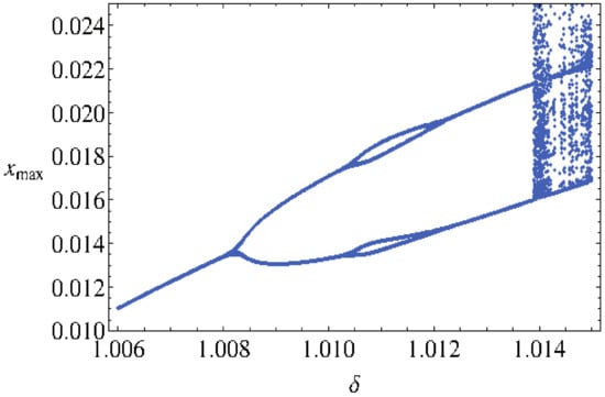
Figure 1.
Bifurcation diagram as function of .
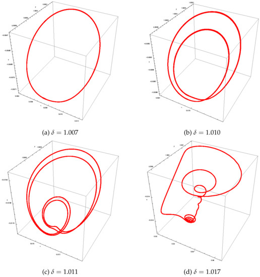
Figure 2.
Phase portraits of system (1) in the phase space for various values .
From Figure 1, we observe that, for , the attractor is a limit cycle of period one (see Figure 2a). For and , the period of the limit cycle becomes of period two (see Figure 2b). For , the limit cycle is of period four (see Figure 2c). When , the attractor becomes chaotic (see Figure 2d). To confirm these results, Lyapunov characteristic exponents were computed in each case.
3.3. Numerical Computation of the Lyapunov Characteristic Exponents
The numerical computation of the Lyapunov characteristic exponents (LCEs) of the system (1) was performed in each case with the algorithm developed by Sandri [30] for Mathematica and the Lyapunov Exponents Toolbox (LET) developed by Siu for MatLab and involving the two algorithms proposed by Wolf et al. [31] and Eckmann and Ruelle [32] (see https://fr.mathworks.com/matlabcentral/fileexchange/233-let 15 September 2021). The results obtained by both algorithms are consistent. The LCE values were computed within each considered interval . As an example, for and , both algorithms provided, respectively, the following LCEs: , , and . Then, the classification of (autonomous) continuous-time attractors of the dynamical system (6) on the basis of their Lyapunov spectrum, together with their Hausdorff dimension, is presented in Table 1 according to the work of Klein and Baier [33].

Table 1.
Lyapunov characteristic exponents of dynamical system (6) for various values of .
4. Slow Invariant Manifold
In recent publications, a new approach to n–dimensional singularly perturbed systems of ordinary differential equations, called the Flow Curvature Method, has been developed by Ginoux et al. [22,23,24,25,26,27,34,35,36,37]. It consists of considering the trajectory curves integral of such systems as curves in Euclidean n–space. Based on the use of local metric properties of curvatures inherent to Differential Geometry, this method, which does not require the use of asymptotic expansions, states that the location of the points where the local curvature of the trajectory curves of such systems is null defines an –dimensional manifold associated with this system and called the flow curvature manifold. The invariance of this manifold is then stated according to a theorem introduced by Gaston Darboux [38] in 1878. Moreover, as stated in Ginoux [25], if the slow–fast dynamical system has a symmetry such as (), its flow curvature manifold has the same, i.e., . Thus, as previously stated (see Section 2), the system (1) is a three-dimensional singularly perturbed dynamical system with two fast variables. However, in such a specific case, one of the hypotheses of Tikhonov’s theorem [5] is not checked since the fast dynamics of the singular approximation have a periodic solution. Nevertheless, while using the Flow Curvature Method, an approximation up to order three in and of the slow invariant manifold equation of the system (1) can been computed for various values of the bifurcation parameter.
According to the Flow Curvature Method, the following proposition holds for any n-dimensional singularly perturbed dynamical system comprising small multiplicative parameters in its velocity vector field:
Proposition 1.
The location of the points where the curvature of the flow, i.e., the curvature of the trajectory curve integral of any n–dimensional singularly perturbed dynamical systems vanishes, providing a p-order approximation of its slow manifold, the equation of which reads
where represents the time derivatives up to order n of the velocity vector field.
For a proof of this proposition and that of the invariance of the slow manifold (14), see Ginoux [22,23,24,25,26,27,28,34]. Let us observe that the p-order approximation depends on the number of small multiplicative parameters in the velocity vector field. In the particular case of system (1), it can be easily stated that, since the plane is invariant with respect to the flow and due to the presence of two small multiplicative parameters, i.e., and , the slow invariant manifold Equation (14) can be simply and directly expressed by:
where is the unit vector along the x-axis. Thus, by using the Flow Curvature Method and Equation (15), the slow invariant manifold equation of system (1) reads:
The slow invariant manifold equations (16) of the system (1) have been plotted in the figures below (see Figure 3) for various values of the bifurcation parameter and .
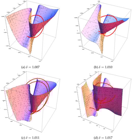
Figure 3.
Slow invariant manifolds of system (1) in the phase space for various values of .
We observe that, for , the trajectory curve integral of system (1) is a periodic stable limit cycle that lies partly on the left side and right side of the slow invariant manifold; see Figure 3a. For a bifurcation parameter equal to and (see Figure 3b,c), the same evolution appears. Let us observe that the kind of funnel in Figure 3a,c corresponds to the attractive eigendirection of the fixed point . When , the attractor becomes chaotic and the trajectory curve evolves slowly from the bottom to the top on nearly all the left part of the slow invariant manifold. Then, it jumps on the upper right part of slow invariant manifold and starts spiraling around the attractive eigendirection corresponding to the negative real eigenvalues of fixed point ; see Equations (9) and (10). When the trajectory curve reaches the lower right part of the slow invariant manifold, it jumps on its left part. Let us observe that, during its descent, it lies in the vicinity of the slow invariant manifold; see Figure 3d and Figure 4.
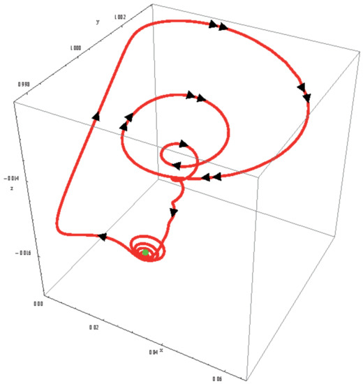
Figure 4.
Evolution of the trajectory curve integral of system (1) for .
5. Discussion
In this work, by using the so-called Flow Curvature Method, we provide the slow invariant manifold analytical equation of a laser model. This equation and its graphical representation in the phase space enable, on the one hand, discriminating the slow evolution of the trajectory curves from the fast one and, on the other hand, improving our understanding of this slow–fast regime. Thus, the repelling and attracting branches of the slow invariant manifold have been specified. We also highlighted that the deformation of the surface representing, in the phase space (x, y, z), the slow invariant analytical manifold according to the bifurcation parameter is rather weak (see Figure 3). This confirms an assumption made by Al-Naimee et al. [1] according to which:
“Therefore, it is expected that they should not imply strong modifications of the slow-manifold shape which, as discussed above, is responsible for the observed dynamics.”
Finally, our mathematical analysis also enabled confirming another assumption made by Al-Naimee et al. [1], according to which “since () is located precisely on the slow manifold, the exact homoclinic connection does not occur”.
Author Contributions
Conceptualization, J.-M.G. and R.M. Both authors have equally contributed. All authors have read and agreed to the published version of the manuscript.
Funding
This research received no external funding.
Conflicts of Interest
The authors declare no conflict of interest.
References
- Al-Naimee, K.; Marino, F.; Ciszak, M.; Meucci, R.; Arecchi, F.T. Chaotic spiking and incomplete homoclinic scenarios in semiconductor lasers with optoelectronic feedback. New J. Phys. 2009, 11, 073022. [Google Scholar] [CrossRef][Green Version]
- Poincaré, H. Les Méthodes Nouvelles de la Mécanique Céleste; Gauthier-Villars: Paris, France, 1892; Volumes I–III. [Google Scholar]
- Andronov, A.A.; Chaikin, S.E. Theory of Oscillators, Moscow, I., English Translation; Princeton University Press: Princeton, NJ, USA, 1949. [Google Scholar]
- Levinson, N. A second-order differential equation with singular solutions. Ann. Math. 1949, 50, 127–153. [Google Scholar] [CrossRef]
- Tikhonov, A.N. On the dependence of solutions of differential equations on a small parameter. Mat. Sb. N.S. 1948, 31, 575–586. [Google Scholar]
- Wasow, W.R. Asymptotic Expansions for Ordinary Differential Equations; Wiley-Interscience: New York, NY, USA, 1965. [Google Scholar]
- Cole, J.D. Perturbation Methods in Applied Mathematics; Blaisdell: Waltham, MA, USA, 1968. [Google Scholar]
- O’Malley, R.E. Introduction to Singular Perturbations; Academic Press: New York, NY, USA, 1974. [Google Scholar]
- O’Malley, R.E. Singular Perturbations Methods for Ordinary Differential Equations; Springer: New York, NY, USA, 1991. [Google Scholar]
- Fenichel, N. Persistence and Smoothness of Invariant Manifolds for Flows. Ind. Univ. Math. J. 1971, 21, 193–225. [Google Scholar] [CrossRef]
- Fenichel, N. Asymptotic stability with rate conditions. Ind. Univ. Math. J. 1974, 23, 1109–1137. [Google Scholar] [CrossRef]
- Fenichel, N. Asymptotic stability with rate conditions II. Ind. Univ. Math. J. 1977, 26, 81–93. [Google Scholar] [CrossRef]
- Fenichel, N. Geometric singular perturbation theory for ordinary differential equations. J. Diff. Eq. 1979, 31, 53–98. [Google Scholar] [CrossRef]
- Hirsch, M.W.; Pugh, C.C.; Shub, M. Invariant Manifolds; Springer: New York, NY, USA, 1977. [Google Scholar]
- Rossetto, B. Trajectoires lentes des syst‘emes dynamiques lents-rapides. In Analysis and Optimization of System; Springer: Berlin/Heidelberg, Germany, 1986; pp. 680–695. [Google Scholar]
- Rossetto, B. Singular approximation of chaotic slow-fast dynamical systems. In The Physics of Phase Space Nonlinear Dynamics and Chaos Geometric Quantization, and Wigner Function; Springer: Berlin/Heidelberg, Germany, 1987; pp. 12–14. [Google Scholar]
- Gear, C.W.; Kaper, T.J.; Kevrekidis, I.G.; Zagaris, A. Projecting to a slow manifold: Singularly perturbed systems and legacy codes. SIAM J. Appl. Dyn. Syst. Math. 2005, 4, 711–732. [Google Scholar] [CrossRef]
- Zagaris, A.; Gear, C.W.; Kaper, T.J.; Kevrekidis, Y.G. Analysis of the accuracy and convergence of equation-free projection to a slow manifold. ESAIM Math. Model. Num. 2009, 43, 757–784. [Google Scholar] [CrossRef]
- Maas, U.; Pope, S.B. Simplifying chemical kinetics: Intrinsic low-dimensional manifolds in composition space. Combust. Flame 1992, 8, 239–264. [Google Scholar] [CrossRef]
- Brøns, M.; Bar-Eli, K. Asymptotic analysis of canards in the EOE equations and the role of the inflection line. Proc. R. Soc. Lond. Ser. A Math. Phys. Eng. Sci. 1994, 445, 305–322. [Google Scholar]
- Rossetto, B.; Lenzini, T.; Ramdani, S.; Suchey, G. Slow fast autonomous dynamical systems. Int. J. Bifurc. Chaos 1998, 8, 2135–2145. [Google Scholar] [CrossRef]
- Ginoux, J.M.; Rossetto, B. Slow manifold of a neuronal bursting model. In Emergent Properties in Natural and Articial Dynamical Systems; Aziz-Alaoui, M.A., Bertelle, C., Eds.; Springer: Berlin/Heidelberg, Germany, 2006; pp. 119–128. [Google Scholar]
- Ginoux, J.M.; Rossetto, B. Differential Geometry and Mechanics Applications to Chaotic Dynamical Systems. Int. J. Bif. Chaos 2006, 4, 887–910. [Google Scholar] [CrossRef]
- Ginoux, J.M.; Rossetto, B.; Chua, L.O. Slow Invariant Manifolds as Curvature of the Flow of Dynamical Systems. Int. J. Bif. Chaos 2008, 11, 3409–3430. [Google Scholar] [CrossRef]
- Ginoux, J.M. Differential Geometry Applied to Dynamical Systems; World Scientific Series on Nonlinear Science; Series A 66; World Scientific: Singapore, 2009. [Google Scholar]
- Ginoux, J.M.; Llibre, J. The flow curvature method applied to canard explosion. J. Phys. A Math. Theor. 2011, 44, 465203. [Google Scholar] [CrossRef]
- Ginoux, J.M. The Slow Invariant Manifold of the Lorenz-Krishnamurthy Model. Qual. Theory Dyn. Syst. 2014, 13, 19–37. [Google Scholar] [CrossRef]
- Ginoux, J.M. Slow Invariant Manifolds of Slow-Fast Dynamical Systems. Int. J. Bif. Chaos 2021, 31, 2150112-1-17. [Google Scholar] [CrossRef]
- Bender, C.M.; Orszag, S.A. Advanced Mathematical Methods for Scientists and Engineers; Springer: New York, NY, USA, 1999. [Google Scholar]
- Sandri, M. Numerical Calculation of Lyapunov Exponents. Math. J. 1996, 6, 78–84. [Google Scholar]
- Wolf, A.; Swift, J.B.; Swinney, H.L.; Vastano, J.A. Determining Lyapunov Exponents from a Time Series. Phys. D 1985, 16, 285–317. [Google Scholar] [CrossRef]
- Eckmann, J.P.; Ruelle, D. Ergodic Theory of Chaos and Strange Attractors. Rev. Mod. Phys. 1985, 57, 617–656. [Google Scholar] [CrossRef]
- Klein, M.; Baier, G. Hierarchies of Dynamical Systems. In A Chaotic Hierarchy; Baier, G., Klein, M., Eds.; World Scientific: Singapore, 1991. [Google Scholar]
- Ginoux, J.M.; Llibre, J.; Chua, L.O. Canards from Chua’s circuit. Int. J. Bif. Chaos 2013, 23, 1330010. [Google Scholar] [CrossRef]
- Ginoux, J.M.; Llibre, J. Canards Existence in FitzHugh-Nagumo and Hodgkin-Huxley Neuronal Models. Math. Probl. Eng. 2015, 2015, 342010. [Google Scholar] [CrossRef]
- Ginoux, J.M.; Llibre, J. Canards Existence in Memristor’s Circuits. Qual. Theory Dyn. Syst. 2016, 15, 383–431. [Google Scholar] [CrossRef]
- Ginoux, J.M.; Llibre, J.; Tchizawa, K. Canards Existence in The Hindmarsh-Rose Model. Math. Model. Nat. Phenom. 2019, 14, 1–21. [Google Scholar] [CrossRef]
- Darboux, G. Mémoire sur les équations différentielles algébriques du premier ordre et du premier degré. Bull. Sci. Math. Sér. 1878, 2, 60–96, 123–143, 151–200. [Google Scholar]


Publisher’s Note: MDPI stays neutral with regard to jurisdictional claims in published maps and institutional affiliations. |
© 2021 by the authors. Licensee MDPI, Basel, Switzerland. This article is an open access article distributed under the terms and conditions of the Creative Commons Attribution (CC BY) license (https://creativecommons.org/licenses/by/4.0/).