
Classification of Integrodifferential C∗-Algebras

Department of Mathematics & Logistics, Jacobs University, Campus Ring 1, 28759 Bremen, Germany
Symmetry 2021, 13(10), 1900; https://doi.org/10.3390/sym13101900
Submission received: 6 September 2021
/
Revised: 2 October 2021
/
Accepted: 5 October 2021
/
Published: 9 October 2021
(This article belongs to the Special Issue Mathematical Physics: Topics and Advances)
Abstract
:The infinite product of matrices with integer entries, known as a modified Glimm–Bratteli symbol , is a new, sufficiently simple, and very powerful tool for the characterization of approximately finite-dimensional (AF) algebras. This symbol provides a convenient algebraic representation of the Bratteli diagram for AF algebras in the same way as was previously performed by J. Glimm for more simple uniformly hyperfinite (UHF) algebras. We apply this symbol to characterize integrodifferential algebras. The integrodifferential algebra is the -algebra generated by the following operators acting on : (1) operators of multiplication by bounded matrix-valued functions, (2) finite-difference operators, and (3) integral operators. Most of the operators and their approximations studying in physics belong to these algebras. We give a complete characterization of . In particular, we show that does not depend on M, but depends on N. At the same time, it is known that differential algebras , generated by the operators (1) and (2) only, do not depend on both dimensions N and M; they are all ∗-isomorphic to the universal UHF algebra. We explicitly compute the Glimm–Bratteli symbols (for , it was already computed earlier) which completely characterize the corresponding AF algebras. This symbol is an infinite product of matrices with nonnegative integer entries. Roughly speaking, all the symmetries appearing in the approximation of complex infinite-dimensional integrodifferential and differential algebras by finite-dimensional ones are coded by a product of integer matrices.
1. Introduction
Discrete and continuous analogs of integrodifferential algebras are actively used in various applications, for example, in the development of computer algorithms for symbolic and numerical solving of integrodifferential equations, see, e.g., [1,2,3,4]. These studies do not concern the structure of -algebras. On the other hand, differential algebras are closely related to the rotation -algebras well studied in, e.g., [5,6,7,8]. In contrast to the rotation algebras, the integrodifferential algebras contain operators of multiplication by discontinuous functions and integral operators. Nevertheless, the integrodifferential algebras are AF algebras and, hence, they admit a classification in terms of, e.g., the Bratteli diagrams. We give an algebraic representation of the Bratteli diagrams based on the infinite products of matrices with nonnegative integer entries. These infinite products of matrices extend the infinite products of natural numbers that J. Glimm used for the characterization of uniformly hyper-finite algebras. This is a reason why we call the infinite products of matrices Glimm–Bratteli symbols. GB symbols are a fairly powerful tool because it allows one to use a simple matrix product technique to prove the presence or absence of isomorphism between algebras. In general, isomorphism is very important in understanding the differences and similarities between different classes of operators. Recently, in [9], it was proved that all the differential -algebras are isomorphic, independently of their dimensions. A natural question arises: what will happen if we add integral operators to differential algebras? We see below that the resulting integrodifferential algebras are already nonisomorphic to each other, they depend on the dimension. Thus, while there are unified methods for analyzing finite-difference approximations of differential equations for any dimension, the analysis of such approximations of integrodifferential equations may strongly depend on the dimensions.
The current research is devoted to the integrodifferential operators acting on multidimensional tori. In the future, we plan to adapt the analysis to more complex stochastic integrodifferential operators acting on non-compact and fractal domains.
The manuscript is organized as follows: Section 2 contains basic information about ∗-homomorphisms of finite-dimensional -algebras, a structure of AF-algebras, related graphical Bratteli diagrams along with their algebraic representations by the Glimm–Bratteli symbols, and some examples; Section 3 is devoted to the characterization of integrodifferential -algebras in terms of the Glimm–Bratteli symbols; Section 4 contains the proofs of the results from Section 2 and Section 3; we conclude in Section 5.
2. Characterization of AF-Algebras. Infinite Product of Matrices with Integer Entries
Let us recall some facts about Bratteli diagrams. It is well known that any finite-dimensional -algebra is ∗-isomorphic to the direct sum of simple matrix algebras. Up to the order of terms, this direct sum is determined uniquely. It is convenient to use the following notation for finite-dimensional -algebras. Let , then
Any ∗-homomorphism from to with , is internally (inside each ) unitary equivalent to some canonical ∗-homomorphism. Any canonical ∗-homomorphism is completely and uniquely determined by the matrix of multiplicities of partial embeddings (E matrix), satisfying , where , and . For example, the canonical ∗-homomorphism
has the E matrix
For simplicity, we can write
If a canonical ∗-homomorphism is unital then there are no zero rows in the E matrix, and we should replace the above-mentioned condition with . For example, the unital embedding
has the form
The AF algebra is a separable -algebra, any finite subset of which can be approximated by a finite-dimensional -subalgebra. For convenience, we will consider unital AF algebras only. This is not a restriction because the unitalization of an AF algebra is obviously an AF algebra. It is well known that for any unital AF algebra , there is a family of nested finite-dimensional -subalgebras , satisfying
Since are nested finite-dimensional -algebras, they are isomorphic to some canonical algebras , where , , and the inclusions (2) can be written as
where , , and . Moreover, due to the unital embeddings , all E matrices have no zero rows and columns and they satisfy . Because , we obtain
We will always assume the right-to-left order in the product ∏. Using (3) and (4), we conclude that the matrices completely determine the structure of the unital AF algebra . It is useful to note that the choice of E matrices is not unique. For example, E matrices , where , determine the same algebra . This is because the composition of two embeddings has the E-matrix equivalent to the product of E matrices corresponding to the embeddings. It is possible to describe the class of all E-matrices determining the same unital AF-algebra.
Definition 1.
Let be the set of sequences of matrices , where have no zero rows and columns, and , are some positive integer numbers. Let us define the equivalence relation on . Two sequences are equivalent if there is such that
where and are some monotonic sequences of integer numbers. The corresponding set of equivalence classes is denoted by .
It is convenient to denote the equivalence classes as
because, see (5),
In other words, we can perform the standard manipulations in the product of matrices without leaving the equivalence class. Of course, the manipulations should not go beyond , i.e., all the resulting matrices should have non-negative integer entries and should not have zero rows and zero columns.
Let be a unital AF algebra. Following (2)–(4), there is , which represents a Bratteli diagram for . Let us define the mapping
Because the Bratteli diagram is not unique, the correctness of the mapping should be checked. This is already complete in the main structure theorem for Bratteli diagrams.
Theorem 1.
(i) The relation ∼ defined in Definition 1 is the equivalence relation. (ii) Let be the set of classes of nonisomorphic unital A -algebras. Then, is 1–1 mapping.
Note that the inverse mapping has a more explicit form than . For example, is the -algebra given by the inductive limit (3).
The proof of Theorem 1 follows from the similar results formulated for the graphical representations of Bratteli diagrams, see, e.g., [10,11], and Theorem 3.4.4 in [12]. The equivalence relation ∼ is the complete analogue of telescopic transformations of Bratteli diagrams defined in [12]. While the Bratteli diagram is not unique, it provides a kind of good classification tool. Other types of classification of AF algebras, including the efficient K-theoretic Elliott classification, are discussed in [13,14,15,16,17]. The infinite product representing the Bratteli diagram for AF-algebra can be called the Glimm–Bratteli symbol. The reason for using this name is the following. Working with supernatural symbols (numbers), when are natural numbers in (6), J. Glimm provides the classification of UHF algebras in [18]. In turn, the UHF algebras are a partial case of AF algebras for which the supernatural numbers should be replaced with “supernatural matrices” connected with the corresponding Bratteli diagram. Let us consider some examples of AF algebras.
Example 1
(Compact operators). Let be the -algebra of compact operators acting on a separable Hilbert space. Let be its unitalization. It is well known, see, e.g., [12], that the Bratteli diagram for can be presented as it is drawn in Figure 1.
The nodes correspond to simple matrix sub-algebras, and the edges show the multiplicity of embedding: one line means the multiplicity is equal to 1, two lines means the multiplicity is 2, and so on. The first node is a node that has no incoming edges; it is always . The dimensions of nodes are determined by the dimensions of nodes connected on the left and by the multiplicities of embedding. The corresponding Glimm–Bratteli symbol is
Combining terms in the infinite product, we can write another form of the Glimm–Bratteli symbol
which leads to the labeled Bratteli diagram depicted in Figure 2.
In the labeled Bratteli diagram, the edge numbers are the multiplicities of embeddings. The multiplicity 1 is usually omitted.
Example 2
(CAR algebra). For the CAR (canonical anticommutation relations) algebra , which is a UHF algebra, the Glimm–Bratteli symbol is . At the same time,
The corresponding Bratteli diagrams are depicted in Figure 3.
Comparing this explanation with the similar one given in [12], it is seen how the symbol simplifies the proof of equivalence of presented Bratteli diagrams.
Example 3
(Direct sum of AF algebras). Above, we already used the notation ⊕ for the direct sum of matrix algebras and for their elements. We will use the same symbol in a slightly different context, namely for the direct sum of not necessarily square E matrices. Suppose that is the standard direct sum of two AF algebras. If and then it can be shown that
Example 4
(Tensor product of AF-algebras). It is useful to note the following property of the tensor product
where
Moreover, it is easy to check that if
then
where the tensor product of matrices is defined in the standard way
Hence, the standard tensor product of two AF algebras is an AF algebra which satisfies
where , , and the tensor product of matrices is then
We will also use the following result.
Theorem 2.
Let be a commutative (multiplicative) semigroup of square matrices with non-negative integer entries and with non-zero determinants. Let be a matrix column with positive integer entries such that is defined. Let be a subset consisting of not necessarily different matrices satisfying the condition (σ): for any there are such that . Then,
Even if (σ) is not fulfilled, LHS in (7) is a sub-algebra of RHS.
Remark 1.
The universal UHF algebra is the AF algebra generated by the multiplicative semigroup of natural numbers
where , , , … are the prime numbers. Any UHF algebra is a sub-algebra of . The CAR algebra is the UHF algebra generated by any of the following multiplicative semigroups , where .
There is another useful proposition describing nonisomorphic classes of AF algebras.
Theorem 3.
Let . Let , be two sequences of matrices with non-zero determinants. Let , be two matrix columns without zero entries. If , then are nonisomorphic -algebras.
3. Main Results
Let be positive integers. Let be the Hilbert space of periodic vector-valued functions defined on the multidimensional torus , where . Everywhere in the article, it is assumed the Lebesgue measure in the definition of Hilbert spaces of square-integrable functions. Let be the -algebra of matrix-valued regulated functions with rational discontinuities. The regulated functions with possible rational discontinuities are the functions that can be uniformly approximated by the step functions of the form
where , , and is the characteristic function of the parallelepiped with rational end points . In particular, continuous matrix-valued functions belong to . Let us introduce generating operators for the integrodifferential algebras. These operators are operators of multiplication by a function , finite-difference operators , and integral operators , all of which act on :
where the function , the index , the step of differentiation , the standard basis vector , and is the Kronecker symbol. The -algebra of integrodifferential operators is generated by all the operators (9)
where is the -algebra of all the bounded operators acting on . The typical example of an operator from is
where , , and . Let us provide the characterization of .
Theorem 4.
The AF-algebra has the following Glimm–Bratteli symbol
In particular, and are isomorphic if, and only if, .
Integrodifferential algebras with a different number of variables are nonisomorphic. This fact indicates a significant difference between the integrodifferential algebras and differential algebras generated by and . The algebras are all isomorphic to the universal UHF algebra independently on the number of variables N and the number of functions M; see [9].
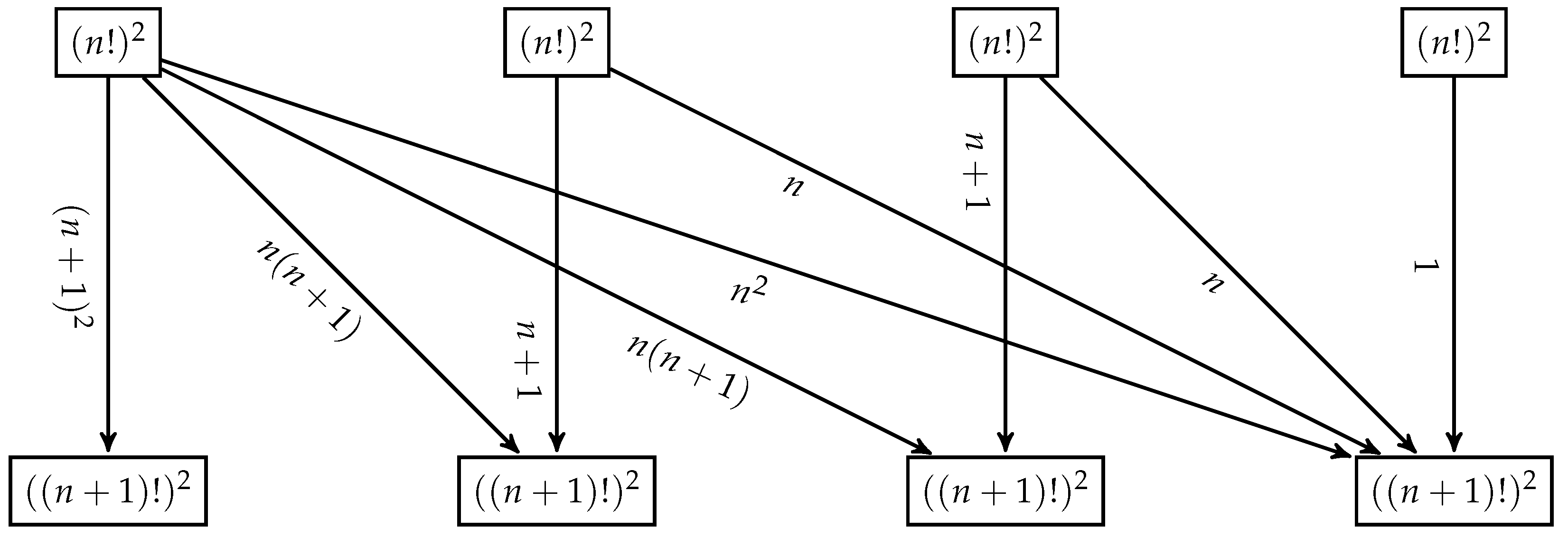
Example 5.
Let us consider the -algebra of two-dimensional integrodifferential operators . We have
and
A fragment of the Bratteli diagram for is depicted in Figure 4. Here, the vertices in the row represent direct summands of the finite-dimensional sub-algebra, the edges represent partial embeddings into the next finite-dimensional sub-algebra appearing in the direct limit, and the edge labels are multiplicities of partial embeddings. Note that the orientation of the Bratteli diagram for is up→down, but the Bratteli diagrams for the examples in the previous section are oriented as left→right. The only reason for that is the convenience of the corresponding graphic illustration.
Remark 2.
Let us consider the algebra of one-dimensional scalar integrodifferential operators . The E matrices for are given by Theorem 4
It is clear that
Thus, there are arbitrary large elements , in . Remembering that these elements correspond to the unitalized algebra of compact operators , see above and, e.g., Example 3.3.1 in [12], we can expect that . This is true because any compact operator can be uniformly approximated by finite-dimensional operators in some orthonormal basis of . Taking the Walsh basis , consisting of step functions, we see that for any , the one-rank operator given by , where , belongs to . Hence, any compact operator belongs to , since it can be uniformly approximated by linear combinations of .
Finally, note that . E matrices for correspond to the universal uniformly hyper-finite algebra which has the supernatural number . As is shown in [9], the algebra , generated by and , see (9), is a sub-algebra of . Thus, roughly speaking, is a combination of the universal UHF algebra and the algebra of compact operators .
The natural extension of (or ) is the AF algebra generated by the following commutative semigroup
This is the maximal commutative semigroup of matrices from with the eigenvectors and . Perhaps it would be interesting to see the “physical meaning” of extended integrodifferential operators from .
4. Proof of the Main Results
Proof of Theorem 2.
The conditions of Definition 1 will be checked. We set , , and , correspondingly. Next, for some . We take , or if . In the first case, we set ; in the second case we set .
Anyway, , since this is a semigroup. Hence, for some , we have by the condition (σ). Thus, because is invertible, and all the matrices are commute. In general, commutativity greatly simplifies the reasoning, since we do not need to worry about the order of the factors.
By induction, suppose that for some , we already found , and , and , satisfying
Let be the maximal element of the matrix . It is true that
since , are matrices with non-negative integer entries, without zero rows and columns. There are two possibilities: (a) , and (b) are bounded. In the case of (a), for some sufficiently large , we have , where . We set , . Hence, we obtain
Note that , since this is a semigroup. Another possibility: (b) are uniformly bounded for all p. Then, for some because is a sequence of matrices with bounded non-negative integer entries. The existence of inverse matrix leads to being the identity matrix. We set , . These values also satisfy (14). Note that matrices satisfying condition (b) correspond to a permutation of elements in the Bratteli diagrams.
Again, there are two possibilities: (a) , and (b) are bounded. Consider the first case (a), the second case (b) can be treated as above. There is , such that
Hence, by the condition (), taking (recall that the set is a semigroup), we have
for some, because of (13) and (15). We set . Using (16), we deduce that
Thus, by induction we prove that and are equivalent; see Definition 1. By Theorem 1, they represent the same algebra.
If are bounded for all p, then there is and such that for all n. Thus, is a sub-algebra of , which, in turn, is the sub-algebra of . Now, suppose that . Then, we can take such that
where , denoting
where is the identity matrix if . Then, the following infinite commutative diagrams
show that is the sub-algebra of . □
Proof of Theorem 3.
Suppose that . If ; then, there is a sequence of matrices satisfying (5), namely
for some . This yields to
The matrix in LHS has the full rank N, while the matrix in RHS has a rank less or equal to M. This is the contradiction. □
Proof of Theorem 4.
Let us start from the 1D case . For : define the shift operator . Define also the operators of multiplication by the characteristic functions of intervals
The operators satisfy some elementary properties that can be checked directly; see also [19],
where , , and . For , define the basis operators
Using (19), we can directly check the properties
Identities (21) mean that
with the ∗-isomorphism defined by
where is the zero element in . Let be some positive integer. Using (20) and the identity
we obtain
Identity (24) shows how is embedded into . Namely, the corresponding ∗-embedding is defined by
where is the identity matrix in and is the matrix, which has all entries equal to 1. The matrix is the rank-one matrix with the unit trace and, hence, it is unitarily equivalent to the matrix with one nonzero entry
Using (26), we conclude that ∗-embedding (25) between and has the E matrix
The integral operator belongs to all , since
By definition, any can be uniformly approximated by step functions with rational discontinuities. Thus, the operator of multiplication by the function can be uniformly approximated by linear combinations of , . On the other hand, using (20), we have
Hence, for any , the operator can be uniformly approximated by the elements from with arbitrary precision when . The identity operator 1 belongs to all , since
The shift operators (with ) belongs to , since
by (19), (20) and (30). Hence, the finite differentials belong also to :
Using (28) and (32), and the above-mentioned fact about the approximation of (for any ) by the elements from , we conclude that is the inductive limit of for . In particular, taking and using (27) for , we obtain (11) for .
The algebra has the same Glimm–Bratteli symbol as , since
Let us discuss why the first identity in the last string of (33) is true. The matrices (27) form a commutative (multiplicative) semigroup. Then, the infinite product with one duplicated term in the LHS of (33) obviously satisfies the condition () from Theorem 2. Hence, and are isomorphic. There is also a more intuitive similarity with supernatural numbers
where , , , … are prime numbers and is the prime factorization of M. This similarity with supernatural numbers is possible because all the matrices commute with each other. In this sense, the presented idea is somewhat similar to that one related to supernatural numbers, see [18].
Consider the case . Using the fact that , we deduce that . This means that
which proves (11). Thus, the -algebras and are isomorphic if, and only if, by Theorem 3. □
5. Conclusions
We have considered the Glimm–Bratteli symbol that is a convenient algebraic representation of the Bratteli diagrams for AF algebras in the form of infinite products of matrices with integer entries. We have applied this symbol for the classification of the algebra of integrodifferential operators. In particular, the Glimm–Bratteli symbol allowed us to prove easily that the algebras of integrodifferential operators acting on the tori of different dimensions are nonisomorphic. This is an essential addition to the result proved recently: all the algebras of differential operators are isomorphic to each other, independently to the dimensions of the tori that they act on, see [19]. In the future, we plan to characterize the algebras of operators acting on more complex non-compact domains, including fractal ones. Another interesting research area is the application of modified Glimm–Bratteli symbols to the algebras of stochastic integrodifferential operators.
Funding
This paper is a contribution to the project M3 of the Collaborative Research Centre TRR 181 “Energy Transfer in Atmosphere and Ocean” funded by the Deutsche Forschungsgemeinschaft (DFG, German Research Foundation)—Projektnummer 274762653. This work is also supported by the RFBR (RFFI) grant No. 19-01-00094.
Institutional Review Board Statement
Not applicable.
Informed Consent Statement
Not applicable.
Data Availability Statement
The data that support the findings of this study are available from the corresponding author upon reasonable request.
Conflicts of Interest
The author declares no conflict of interest.
References
- Rosenkranz, M. A new symbolic method for solving linear two-point boundary value problems on the level of operators. J. Symb. Comput. 2005, 39, 171–199. [Google Scholar] [CrossRef] [Green Version]
- Guo, L.; Keigher, W. On differential Rota-Baxter algebras. J. Pure Appl. Algebra 2008, 212, 522–540. [Google Scholar] [CrossRef] [Green Version]
- Bavula, V.V. The algebra of integro-differential operators on an affine line and its modules. J. Pure Appl. Algebra 2013, 217, 495–529. [Google Scholar] [CrossRef] [Green Version]
- Guo, L.; Regensburger, G.; Rosenkranz, M. On integro-differential algebras. J. Pure Appl. Algebra 2014, 218, 456–473. [Google Scholar] [CrossRef] [Green Version]
- Pimsner, M.; Voiculescu, D. Imbedding the irrational rotation C*-algebra into an AF-algebra. J. Oper. Theory 1980, 4, 201–220. [Google Scholar]
- Rieffel, M.A. C*-algebras associated with irrational rotations. Pac. J. Math. 1981, 93, 415–429. [Google Scholar] [CrossRef] [Green Version]
- Yin, H.S. A simple proof of the classification of rational rotation C*-algebras. Proc. Am. Math. Soc. 1986, 98, 469–470. [Google Scholar] [CrossRef]
- Elliot, G.A.; Niu, Z. All irrational extended rotation algebras are AF algebras. Can. J. Math. 2015, 67, 810–826. [Google Scholar] [CrossRef] [Green Version]
- Kutsenko, A. Isomorphism between one-dimensional and multidimensional finite difference operators. Commun. Pure Appl. Anal. 2021, 20, 359–368. [Google Scholar] [CrossRef]
- Bratteli, O. Inductive limits of finite dimensional C*-algebras. Trans. Am. Math. Soc. 1972, 171, 195–234. [Google Scholar] [CrossRef] [Green Version]
- Davidson, K. C*-Algebras by Example. In Fields Institute Monographs; American Mathematical Society: Providence, RI, USA, 1997. [Google Scholar]
- Nyland, P.K. Bratteli Diagrams; Norwegian University of Science and Technology: Trondheim, Norway, 2016. [Google Scholar]
- Elliot, G.A. On the classiffication of inductive limits of sequences of semisimple finite-dimensional algebras. J. Algebra 1980, 38, 29–44. [Google Scholar] [CrossRef] [Green Version]
- Effros, E.G.; Handelman, D.E.; Shen, C.-L. Dimension groups and their affine representations. Am. J. Math. 1980, 102, 385–407. [Google Scholar] [CrossRef]
- Rordam, M.; Larsen, F.; Laustsen, N.J. An Introduction to K-Theory for C*-Algebras; Cambridge University Press: Cambridge, UK, 2000. [Google Scholar]
- Amini, M.; Elliott, G.A.; Golestani, N. The category of Bratteli diagrams. Can. J. Math. 2015, 67, 990–1023. [Google Scholar] [CrossRef] [Green Version]
- Ghasemi, S.; Kubis, W. Universal AF-algebras. J. Funct. Anal. 2020, 279, 108590. [Google Scholar] [CrossRef]
- Glimm, J.G. On a certain class of operator algebras. Trans. Am. Math. Soc. 1960, 95, 318–340. [Google Scholar] [CrossRef]
- Kutsenko, A.A. Matrix representations of multidimensional integral and ergodic operators. Appl. Math. Comput. 2020, 369, 124818. [Google Scholar] [CrossRef] [Green Version]
Figure 1.
Bratteli diagram for the unitalized -algebra of compact operators .
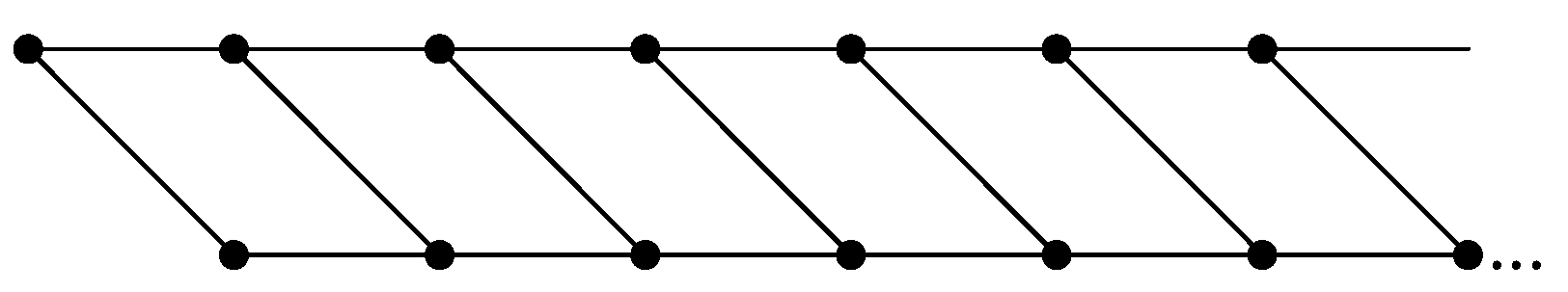
Figure 2.
Another variant of the Bratteli diagram for the unitalized -algebra of compact operators .
Figure 2.
Another variant of the Bratteli diagram for the unitalized -algebra of compact operators .
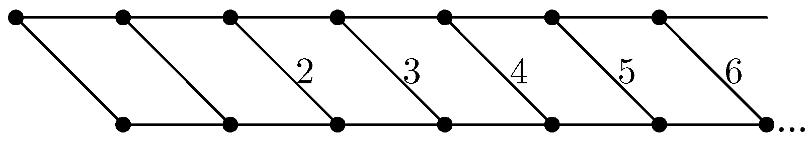
Figure 3.
Different Bratteli diagrams represent the same -algebra .

Figure 4.
The fragment of Bratteli diagrams for -algebra .
Publisher’s Note: MDPI stays neutral with regard to jurisdictional claims in published maps and institutional affiliations. |
© 2021 by the author. Licensee MDPI, Basel, Switzerland. This article is an open access article distributed under the terms and conditions of the Creative Commons Attribution (CC BY) license (https://creativecommons.org/licenses/by/4.0/).
Share and Cite
MDPI and ACS Style
Kutsenko, A.A. Classification of Integrodifferential C∗-Algebras. Symmetry 2021, 13, 1900. https://doi.org/10.3390/sym13101900
AMA Style
Kutsenko AA. Classification of Integrodifferential C∗-Algebras. Symmetry. 2021; 13(10):1900. https://doi.org/10.3390/sym13101900
Chicago/Turabian StyleKutsenko, Anton A. 2021. "Classification of Integrodifferential C∗-Algebras" Symmetry 13, no. 10: 1900. https://doi.org/10.3390/sym13101900
Note that from the first issue of 2016, this journal uses article numbers instead of page numbers. See further details here.