Fast Computation of Green Function for Layered Seismic Field via Discrete Complex Image Method and Double Exponential Rules

Abstract

A novel computational method to evaluate the Sommerfeld integral (SI) efficiently and accurately is presented. The method rewrites the SI into two parts, applying discrete complex image method (DCIM) to evaluate the infinite integral while using double exponential quadrature rules (DE rules) for the computation of the finite part. Estimation of signal parameters via rotational invariance techniques (ESPRIT) is used to improve the accuracy and efficiency of extracting DCIM compared to the generalized pencil of function (GPOF). Due to the symmetry of the horizontal layered media, the Green function, representing the seismic fields due to a point source, can be written in the form of Sommerfeld integral in cylindrical coordinate system and be calculated by the proposed method. The performance of the method is then compared to the DE rules with weighted average partition extrapolation (WA), which shows a good agreement, with computational time reduced by about 40%.

1. Introduction

Green function for the horizontal layered seismic field is usually derived by reflectivity method, which was proposed by Fuchs and Müller [1] and extended to many other kinds [2], like reflection and transmission coefficient matrix method [3], discrete wavenumber method [4], discrete wavenumber finite element method [5], and generalized reflection transmission coefficient matrix method [6]. In the frequency domain, the Green function, derived by the reflectivity method, can be written in the Sommerfeld integral form in cylindrical coordinate system for symmetrical media.

It is well known that the numerical evaluation of Sommerfeld integral (SI) is computationally expensive due to the oscillatory and slow convergence of the integrands. To overcome this problem, several approaches have been proposed, which can be divided into two main categories: one is the approximation of the spatial domain Green functions in a closed form where no numerical integration is needed, and the other is the numerical integration of SI in conjunction with some acceleration techniques [7]. Within the first category, discrete complex image method (DCIM), which approximates the integrand of Sommerfeld integral by a series of complex exponential functions, is commonly used for the advantages of high computational efficiency, but it needs to handle the surface wave poles contributions, which not only makes the computation complicated but also brings singularity to the near region [8], and also the calculation accuracy and effective range are difficult to be accurately estimated. For the latter category, the common practice is dividing the whole Sommerfeld integral into two parts: the first part is the path to bypass the singularity; the second part, the path to infinity, is the Sommerfeld tail integral. The finite-range integrals may readily be evaluated by the Gauss–Jacobi quadrature [9] or by the double-exponential (DE) rule [10,11]. Mosig first used DE rules to calculate Sommerfeld integrals in [11,12] which indicated its validity of suppressing endpoint singularities. The calculation of tail integral is difficult to converge due to Bessel’s oscillation and slow attenuation characteristics, so this kind of method generally requires extrapolation to accelerate convergence. The WA method has shown higher levels of convergence among various extrapolation methods [13,14,15]. This kind of method does not need to strictly locate the position of singularity in Sommerfeld integral but only needs to ensure that the first integral path avoids all the singularities. It has good adaptability and controllable numerical accuracy; however, this depends on the number of intervals (n) that are chosen to evaluate the tail region. The computational time also rapidly increases as the value of (n) increases [16]. Given the advantages and disadvantages of these two methods, we propose a method by combining DE rules and DCIM to calculate Sommerfeld integral.

This paper first presents the Green function of a point source in a multilayer half-space in Section 3, explaining the mathematical manipulation required to obtain the solution as a Sommerfeld integral form in the frequency domain; it then describes the principle of the proposed method with DE quadrature rules and DCIM in Section 4; finally, it corroborates the correctness of the algorithm by the frequency responses obtained from the proposed approach with those where DE rules and WA partition-extrapolation are used for half-space model, and the finite element method is used for three layers model.

2. Seismic Wave Equation and Green Function

2.1. Seismic Wave Equation

The propagation of seismic wavefield in the time domain can be simplified by the following three-dimensional acoustic wave equation:

$${\nabla }^{2}u(x,y,z,t)=\frac{1}{v{(x,y,z)}^2}\frac{{\partial }^{2}u(x,y,z,t)}{\partial t^2}+f(x,y,z,t)$$

(1)

where $u (x,y,z,t)$, $v (x,y,z,t)$, and $f(x,y,z,t)$ represent displacement, velocity, and source term, respectively. $f(x,y,z,t)=-\delta (x-x_s,y-y_s,z-z_s)s(t)$, $s(t)$ is the wavelet, and Ricker wavelet is used in this paper; and $\delta (x-x_s,y-y_s,z-z_s)$ is the Dirac function at the source point $(x_s,y_s,z_s)$.

By Fourier-transform of Equation (1), the two-dimensional acoustic wave equation in frequency domain is obtained, and therefore, Green function for the problem is defined by the following equation:

$${\nabla }^{2}G(x,y,z,\omega )+k^{2}G(x,y,z,\omega )=F(x,y,z,\omega )$$

(2)

where, $G$ denotes the Green function, $F(x,y,z,\omega )=-\delta (x-x_s,y-y_s,z-z_s)S(\omega )$ is the source term in the frequency domain, $k(x,y,z)=\omega /v$ is wave number, $S(\omega )$ is Ricker wavelet in the frequency domain, and $\omega$ is the angular frequency.

However, the underground medium is always viscous, which leads to wave energy loss and phase change in the process of propagation. The visco-acoustic wave equation is established to better describe the propagation of the seismic waves in this viscous medium, which is the same form as Equation (2), but the complex velocity is introduced to simulate the viscous effect [17,18,19]. The reciprocal of complex velocity is defined as $\frac{1}{\tilde{v}}=\frac{1}{v}\left(1-\frac{\mathrm{j}}{2Q}\right)$ [18], where $Q$ is quality factor, so the complex wavenumber is set to be $k=\frac{\omega }{v}\left(1-\frac{\mathrm{j}}{2Q}\right)$, $\mathrm{j}=\sqrt{-1}$. In this paper, the value $Q$ generated by Li Qingzhong’s empirical formula is used for numerical simulation [20]

$$Q=14\times {(v/1000.0)}^{2.2}$$

(3)

2.2. Green Function in Full-Space

The Green function of Equation (2) in homogeneous full-space can be expressed as

$$G(x,y,z,\omega )=\frac{S(\omega )e^{-\mathrm{i}{k}_{1}R}}{4\pi R}$$

(4)

where $R=\sqrt{{(x-x_s)}^2+{(y-y_s)}^2+{(z-z_s)}^2}$, $S(\omega )$ is Ricker wavelet in the frequency domain, $\omega$ is the angular frequency, and $k_1$ is the wavenumber of the medium. The above formula can be rewritten in the Sommerfeld integral form in cylindrical coordinate system:

$$\frac{S(\omega )e^{-\mathrm{i}{k}_{1}R}}{4\pi R}=\frac{S(\omega )}{4\pi }{\displaystyle {\mathrm{\int }}_0^{\infty }\frac{m}{m_1}}{e}^{-m_1\left|z-z_s\right|}{J}_0(mr)dm$$

(5)

where $r=\sqrt{{(x-x_s)}^2+{(y-y_s)}^2}$, $m_1=\sqrt{m^2-k_1{}^2}$.

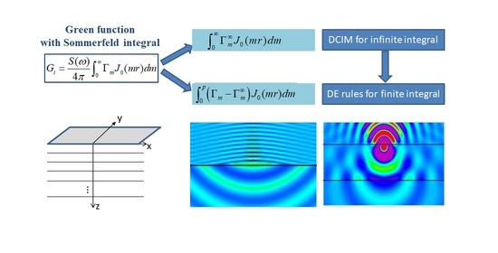
2.3. Green Function in Layered Half-Space

Consider n layers symmetric structure of homogeneous medium defined by interfaces located at $z_1,z_2,\cdots ,z_{n-1}$, as shown in Figure 1. The density of each layer is ${\rho }_1,{\rho }_2,\cdots ,{\rho }_n$; and the velocity is $v_1,v_2,\cdots ,v_n$. In this paper, the source is placed in the second layer.

Each layer satisfies the acoustic Equation (2) with parameters of the Green function $G$, wavenumber $k$, velocity $v$, density $\rho$, layer thickness $h$, and quality factor $Q$, respectively. We obtain the equations as follows:

$${\nabla }^2{G}_i+k_i{}^2{G}_i=0, i=1,3,\cdots ,n$$

(6)

$${\nabla }^2{G}_i+k_i{}^2{G}_i=-S(\omega )\delta (R-R_0) i=2$$

(7)

where $k_i^{}=\frac{\omega }{v_i}\left(1-\frac{\mathrm{j}}{2Q}\right)$, $\mathrm{j}=\sqrt{-1}$.

At the interface, the pressure $P_i={\rho }_i{G}_i$ as well as the gradient of the potential for the vertical direction $\frac{\partial G_i}{\partial z_i}$ are continuous [21]. Therefore, the following boundary conditions can be imposed on the Green function

$$\frac{\partial G_i}{\partial z}=\frac{\partial G_{i+1}}{\partial z},{\rho }_i{G}_i={\rho }_{i+1}{G}_{i+1},(i=1,2,\cdots ,n-1)$$

(8)

The solutions of Equations (6) and (7) can be regarded as the summation of separate up-going and down-going waves, and therefore, it can be written in the form of Sommerfeld integral in cylindrical coordinate system as follows:

$$G_i=\frac{S(\omega )}{4\pi }{\displaystyle {\mathrm{\int }}_0^{\infty }\left(C_i{e}^{m_{i}z}+D_i{e}^{-m_{i}z}\right)}{J}_0(mr)dm, i=1,3,\cdots ,n$$

(9)

$$G_i=\frac{S(\omega )}{4\pi }\left[\frac{e^{-\mathrm{i}{k}_{i}R}}{R}+{\displaystyle {\mathrm{\int }}_0^{\infty }\left(C_i{e}^{m_{i}z}+D_i{e}^{-m_{i}z}\right)}{J}_0(mr)dm\right], i=2$$

(10)

where $m_i=\sqrt{m^2-k_i^2} , k_i^2=\frac{{\omega }^2}{{\tilde{v}}_i{}^2},{\tilde{v}}_i=v_i\left(1-\frac{\mathrm{j}}{2Q_n}\right),i=1,2,\cdots ,n$, $\mathrm{j}=\sqrt{-1}$. In Equations (9) and (10), $e^{m_{i}z}$ and $e^{-m_{i}z}$ may be infinity. To maintain numerical stability, rewrite Equations (9) and (10) into

$$G_i=\frac{S(\omega )}{4\pi }{\displaystyle {\mathrm{\int }}_0^{\infty }\left(C_i{e}^{m_i(z-z_i)}+D_i{e}^{-m_i(z-z_{i-1})}\right)}{J}_0(mr)dm, i=1,3,\cdots ,n$$

(11)

$$G_i=\frac{S(\omega )}{4\pi }\left[\frac{e^{-\mathrm{i}{k}_{i}R}}{R}+{\displaystyle {\mathrm{\int }}_0^{\infty }\left(C_i{e}^{m_i(z-z_i)}+D_i{e}^{-m_i(z-z_{i-1})}\right)}{J}_0(mr)dm\right], i=2$$

(12)

By using the boundary conditions (8), the unknowns $C_1,C_2,D_2,\cdots ,C_i,D_i,\cdots ,$$C_{n-1},D_{n-1},D_n$ in the above formula are solved. The coefficients of the source layer are derived firstly, and other coefficients can be obtained by recursion; then, the expression of the Green function of the layered medium is obtained.

$$D_2=\frac{m}{m_2}\frac{H_2^{d*}\left(H_3^{u\ast }{e}^{-m_2\left|z_2-z_s\right|}{e}^{-m_2{h}_2}-e^{-m_2\left|z_1-z_s\right|}\right)}{1-H_3^{u\ast }{H}_2^{d*}{e}^{-2m_2{h}_2}}$$

(13)

$$C_2=-H_3^{u\ast }\left(\frac{m}{m_2}{e}^{-m_2\left|z_2-z_s\right|}+D_2{e}^{-m_2{h}_2}\right)$$

(14)

$$D_i=\frac{D_{i-1}{m}_{i-1}{e}^{-m_{i-1}{h}_{i-1}}\left(1+H_i^{u\ast }\right)}{m_i\left(1+H_{i+1}^{u\ast }{e}^{-2m_i{h}_i}\right)}$$

(15)

$$C_i=-H_{i+1}^{u\ast }{D}_i{e}^{-m_i{h}_i}$$

(16)

where $h_i=z_{i+1}-z_i$, $H_2^d=\frac{{\rho }_1{m}_2}{{\rho }_2{m}_1}$, $H_2^{d*}=\frac{1-H_2^d}{1+H_2^d}$, $H_n^u=\frac{{\rho }_n{m}_{n-1}}{{\rho }_{n-1}{m}_n}$, $H_n^{u\ast }=\frac{\left(1-H_n^u\right)}{\left(1+H_n^u\right)}$, $H_{i+2}^{u\ast }=\frac{\left(1-H_{i+2}^u\right)}{\left(1+H_{i+2}^u\right)}$, $H_{i+2}^u=\frac{{\rho }_{i+2}{m}_{i+1}}{m_{i+2}{\rho }_{i+1}}\frac{\left(1-H_{i+3}^{u\ast }{e}^{-2m_{i+2}{h}_{i+2}}\right)}{\left(1+H_{i+3}^{u\ast }{e}^{-2m_{i+2}{h}_{i+2}}\right)}$, $i=3,\cdots ,n-1$.

3. Methods

The expressions (11) and (12) contain Sommerfeld integrals, which is an infinite integral with the highly oscillatory and slow-decaying kernel. In this paper, the partial closed form of Sommerfeld integral is derived, and ESPRT is applied to extract DCIM, while DE rules are used for the computation of the finite integration.

3.1. Partial Closed Form Expression

The Sommerfeld integration in Equations (11) and (12) can be written in the following form:

$$I={\displaystyle {\mathrm{\int }}_0^{\infty }\frac{m}{m_i}g(m_i)}{e}^{-m_i\left|z-z_s\right|}{J}_0(mr)dm={\displaystyle {\mathrm{\int }}_0^{\infty }{\mathrm{\Gamma }}_m}{J}_0(mr)dm$$

(17)

The integration is then divided into two parts,

$${\displaystyle {\mathrm{\int }}_0^{\infty }{\mathrm{\Gamma }}_m}{J}_0(mr)dm={\displaystyle {\mathrm{\int }}_0^p{\mathrm{\Gamma }}_m}{J}_0(mr)dm+{\displaystyle {\mathrm{\int }}_p^{\infty }{\mathrm{\Gamma }}_m^{}}{J}_0(mr)dm$$

(18)

where p is a reasonably selected integral breakpoint. The second integral on the right side of the Equation (18) can be asymptotically approximated and then be written as

$${\displaystyle {\mathrm{\int }}_p^{\infty }{\mathrm{\Gamma }}_m^{}}{J}_0(mr)dm\approx {\displaystyle {\mathrm{\int }}_0^{\infty }{\mathrm{\Gamma }}_m^{\infty }}{J}_0(mr)dm-{\displaystyle {\mathrm{\int }}_0^p{\mathrm{\Gamma }}_m^{\infty }}{J}_0(mr)dm$$

(19)

On substituting (19) in (18), we get

$$I\approx {\displaystyle {\mathrm{\int }}_0^p\left({\mathrm{\Gamma }}_m-{\mathrm{\Gamma }}_m^{\infty }\right)J_0(mr)dm}+{\displaystyle {\mathrm{\int }}_0^{\infty }{\mathrm{\Gamma }}_m^{\infty }{J}_0(mr)dm}$$

(20)

The kernel function $g(m_i)$ in (17) can be approximated by an exponential function,

$${\mathrm{\Gamma }}_m^{\infty }=g(m_i)\cdot \frac{m}{m_i}{e}^{-m_i\left|z-z^{\prime }\right|}={\displaystyle \sum _{l=1}^{pb}a(l)}\exp \left[b(l)m_i\right]\cdot \frac{m}{m_i}{e}^{-m_i\left|z-z^{\prime }\right|}$$

(21)

where $pb$ is the number of exponentials used for approximation. In this paper, the coefficients $a (l)$, $b (l)$ are solved by the ESPRIT algorithm, which will be discussed in the next section.

From the Sommerfeld identity expressed by formula (5), the closed form of the second integral can be obtained,

$${\displaystyle {\mathrm{\int }}_0^{\infty }{\mathrm{\Gamma }}_m^{\infty }}{J}_0(mr)dm={\displaystyle \sum _{l=1}^{pb}a (l)}\frac{\exp (-\mathrm{j}{k}_i{R}_l)}{R_l}$$

(22)

where $R_l=\sqrt{r^2+{\left[b (l)-\left|z-z_s\right|\right]}^2}$,

$r=\sqrt{{(x-x_s)}^2+{(y-y_s)}^2}$, $(x_s,y_s,z_s)$ is the location of the source.

The first part of the $g(m_i)$ function usually contains singularity, and the tail is smooth and decays fast. Therefore, if the appropriate p value is selected, the approximate fitting will be very accurate by avoiding the singular value in the front part. The finite integral with singularity in (20) can be evaluated directly by the numerical integration method. We choose DE quadrature rules here for integration with the advantage of dealing with singular points and high precision.

3.2. ESPRIT Algorithm

The signal $g(m_i)$ can be sampled as [8]

$$m_i=k_i\left[T_{02}+\frac{T_{01}-T_{02}}{T_{01}}t\right],0\le t\le T_{01}$$

(23)

The value of $T_{01}$ can be selected from 100~200, $T_{02}$ usually set between 1~3, and in this paper, $T_{01}=200$, $T_{02}=2$, $t$ is an integer. According to the relationship $m^2=m_i^2+k_i^2$, the first sampling in m-plane is $k_i\sqrt{1+T_{02}^2}$. Therefore, the approximation of $g(m_i)$ starts from $m=k_i\sqrt{1+T_{02}^2}$, and the parameter $p$ in formula (20) should be set not less than $k_i\sqrt{1+T_{02}^2}$ to insure the integration accuracy.

Then the sampling sequence can be expressed as

$$g(m_i)=y(t)\approx {\displaystyle \sum _{l=1}^{pb}A (l)\exp \left[B (l)t\right]}$$

(24)

The relation of $A(l)$, $B(l)$, and $a (l)$, $b (l)$ can be obtained from Equations (23) and (24).

$${\displaystyle \sum _{l=1}^{pb}a (l)}\exp \left[b (l)m_i\right]={\displaystyle \sum _{l=1}^{pb}A(l)}\exp \left[B(l)t\right]$$

(25)

Then, the unknown coefficients $a (l)$, $b (l)$ in (24) are obtained.

$$b (l)=\frac{B (l)T_{01}}{k_i(T_{01}-T_{02})}$$

(26)

$$a (l)=A (l)\exp \left(b (l)\cdot k_i\cdot T_{02}\right)$$

(27)

For the sampling sequence $y(0),y(1),\cdots ,y(N-1)$, a data matrix can be constructed:

$$Y={\left[\begin{array}{cccc}y(0)& y(1)& \cdots & y(L)\\ y(1)& y(2)& \cdots & y(L+1)\\ ⋮& ⋮& \ddots & ⋮\\ y(N-L-1)& y(N-L)& \cdots & y(N-1)\end{array}\right]}_{(N-L)\times (L+1)}$$

(28)

where N is the sample number, L is called the pencil parameter, and its value should be between $N/3$ and $N/2$ [22].The data matrix $Y$ can be decomposed by SVD,

$$Y=U\Sigma V^H=\left[\begin{array}{cc}{U}_s& U_n\end{array}\right]\left[\begin{array}{cc}{\Sigma }_s& 0\\ 0& {\Sigma }_n\end{array}\right]\left[\begin{array}{c}{V}_s^H\\ V_n^H\end{array}\right]$$

(29)

where $U$ is $(N-L)\times (N-L)$ orthogonal matrix, and $V$ is $(L+1)\times (L+1)$ orthogonal matrix, $\Sigma$ is $(N-L)\times (L+1)$ diagonal matrix with main diagonal element ${\sigma }_l$, which is the singular value of matrix $Y$. For signals without noise, $Y$ has pb non-zero singular values ${\sigma }_l$ (l= 1,2,..., pb), and pb represents the highest order of the exponential signal of formula (24). If the signal contains noise, mode number pb can be recorded by setting a minimum threshold for ${\sigma }_l$.

Take out the first pb dominant right singular vectors in $V_s$ matrix to form $(L+1)\times pb$ matrix $V_s^{pb}$.The last line of $V_s^{pb}$ is deleted to obtain $L\times M$ matrix $V_1$; the first line of $V_s^{pb}$ is deleted to get $L\times M$ matrix $V_2$. Construct a matrix $\Psi$ [23]

$$\Psi ={\left(V_1^H{V}_1\right)}^{-1}{V}_1^H{V}_2$$

(30)

Find the eigenvalues ${\lambda }_l$ of the matrix $\Psi$,

$$B (l)=\log \left({\lambda }_{ l}\right), l=1,2,\cdots ,pb$$

(31)

For N sampled signals,

$$\lambda =\left(\begin{array}{cccc}1& 1& \cdots & 1\\ {\lambda }_1& {\lambda }_2& \cdots & {\lambda }_{pb}\\ ⋮& ⋮& ⋮& ⋮\\ {\lambda }_1^{N-1}& {\lambda }_2^{N-1}& \cdots & {\lambda }_{pb}^{N-1}\end{array}\right),Y=\left(\begin{array}{c}y(0)\\ y(1)\\ ⋮\\ y(N-1)\end{array}\right),A=\left[\begin{array}{cccc}A(1)& A(2)& \cdots & A(pb)\end{array}\right]$$

(32)

and

$$Y=\lambda A$$

(33)

According to the least square method, we can obtain

$$A={\left({\lambda }^H\lambda \right)}^{-1}{\lambda }^{H}Y$$

(34)

So far, the coefficients $A (l)$ and $B (l)$ are obtained. According to (22), (26), and (27), the second part of Equation (20) is solved, and the integrand of the first part is gained, and then DE rules are applied to compute the finite integral.

3.3. DE Rules

The double exponential transformation was first proposed by Takahasi and Mori in 1974 [16]. It can be seen from Equations (11)–(16) that the integration kernel is singular at $m_i=k_i$. DE rules are insensitive to endpoint singularity and simple to program since the weights and nodes are easily generated [12].

Consider the following form of integral:

$$I={\displaystyle {\mathrm{\int }}_{-1}^{1}ff(\xi )d\xi }$$

(35)

Let a variable transform:

$$\xi =\phi (t) \mathrm{and} \phi (-\infty )=-1,\phi (+\infty )=1$$

(36)

be applied into (35) so as to change the interval $[-1,1]$ into the infinite interval $[-\infty ,+\infty ]$

$$I={\displaystyle {\mathrm{\int }}_{-\infty }^{+\infty }ff(\phi (t)){\phi }^{\prime }(t)}dt$$

(37)

The DE rules are transformed by the tanh–sinh formula,

$$\phi \left(t\right)=\tanh \left(gs\left(t\right)\right)=\tanh \left(\sinh \left(t\right)\right)$$

(38)

$${\phi }^{\prime }(t)=g{s}^{\prime }(t){\mathrm{sech}}^{2}gs(t)=\frac{\cosh (t)}{{\cosh }^2(\sinh (t))}$$

(39)

The standard trapezoidal rule for numerical integration is applied with h as grid interval when the integral is defined on the interval $[-\infty ,+\infty ]$, and n is the sample point, which is truncated at $\pm N$. Then we can approximate the definite integral via

$$I=h{\displaystyle \sum _{n=-\infty }^{\infty }ff(\phi (nh)){\phi }^{\prime }(nh)}\approx h{\displaystyle \sum _{n=-N}^N{\omega }_{n}ff({\xi }_n)}$$

(40)

with the nodes ${\xi }_k$ and weights ${\omega }_k$ defined as

$${\xi }_n=1-{\delta }_n,{\omega }_n=2g^{\prime }(nh){\delta }_n{(1-q_n)}^{-1}$$

(41)

where

$${\delta }_n=2q_n{(1+q_n)}^{-1},q_n=e^{-2gs(nh)}$$

(42)

For arbitrary integral interval $\left[a,b\right]$ may be mapped onto $\left[-1,1\right]$ by the linear transformation $\xi =\sigma x+\gamma$ with $\sigma =(a-b)/2$, $\gamma =(a+b)/2$, which leads to

$${\displaystyle {\mathrm{\int }}_a^{b}ff(\xi )d\xi }=\sigma {\displaystyle {\mathrm{\int }}_{-1}^{1}ff(\sigma x+\gamma )dx}$$

(43)

Hence, for an arbitrary interval $\left[a,b\right]$, the nodes and weights become $\sigma {\xi }_k+\gamma$ and $\sigma {\omega }_k$, respectively, and (43) is transformed to

$${\displaystyle {\mathrm{\int }}_a^{b}ff(\xi )}d\xi \approx \sigma h\left\{g{s}^{\prime }(0)ff(\gamma )+{\displaystyle \sum _{n=1}^N{\omega }_n\left[ff(a+\sigma {\delta }_n)+ff(b-\sigma {\delta }_n)\right]}\right\}$$

(44)

As with any other quadrature rule, singularities of the integrand near the integration path adversely affect the convergence. However, any singularities on the integration path are easily treated by splitting the integration range so that the singularities are placed at the endpoints [12]. Therefore, the integration path in the first part of Equation (20) should be separated into (45) to ensure the convergence of the integration.

$${\displaystyle {\mathrm{\int }}_0^p\left({\mathrm{\Gamma }}_m-{\mathrm{\Gamma }}_m^{\infty }\right)J_0(mr)dm}=\left({\displaystyle {\mathrm{\int }}_0^{bk}}+{\displaystyle {\mathrm{\int }}_{bk}^p}\right)\left({\mathrm{\Gamma }}_m-{\mathrm{\Gamma }}_m^{\infty }\right)J_0(mr)dm$$

(45)

where breakpoint bk is set to the real part of wavenumber $k_i$ in this paper.

4. Results

In this section, the half-space model is designed to test the correctness of the proposed method by comparing it with DE rules and partition-extrapolation WA algorithm [12], which was well accepted and known as one of the most accurate and efficient ones. Finally, the DE_DCIM method is utilized for the calculation of the Green function of the three-layer model in comparison with the finite element method [24].

4.1. Half-Space

It is assumed that the size of the study area is 1410 m ∗ 1410 m ∗ 710 m; the sampling interval in the horizontal and vertical directions is 10 m, taking the main frequency of 20 Hz Ricker wavelet as the source; and the simulation frequency is 10 Hz (all the study areas in the following are consistent with this study area). Consider a half-space defined by interface $z_1$ = 350 m, with a point source located at $(x_s,y_s,z_s)$ = (710 m, 710 m, 360 m). Assume that the velocity and density parameters are set as $v_1$ = 340 m/s, ${\rho }_1$ = 0.00129 g/cm³, $v_2$ = 2000 m/s, ${\rho }_2$ = 1.5 g/cm³. The integration path is divided into three segments, the breakpoint $bk=\mathrm{real}\left({\omega /\tilde{v}}_i\right)$, and the breakpoint $p$ is set as $k_i\sqrt{1+{(198\ast 5\ast T_{02}^{}/200)}^2}$.

Figure 2 shows the comparison of ESPRIT and GPOF methods to extract DCIM of the lower half-space. $g(m_2)$ is defined by (13) and (14); sampling point t is defined in (23). From Figure 2a, both methods gain a good fit with the original data, but the ESPRIT method is slightly more accurate, with a fitting error less than 0.008, while GPOF [25] is less than 0.014. Further, the time cost in computing half-space DCIM is also presented in

Table 1. Computation time comparison with different methods.

Method	GPOF	ESPRIT
Computation time	0.135 s	0.025 s

, which shows ESPRIT also reduces the calculation time. The more layers there are, the more obvious time saving will be seen.

Figure 3 shows the symmetrical wavefield of $(x,y_s,z)$ plane. Comparing the solution of DE_DCIM and the numerical integration with DE_WA, the relative errors are shown in (c) and (f). Excellent agreement is obtained with a relative error of real part less than $2.5\times {10}^{-3}$ and of image part less than $5.8\times {10}^{-4}$, which assesses the validity of the present method. The calculation time of the half-space with different parameters is shown in

Table 2. Computation time comparison with different parameters (computation of $(x,y_s,z)$ plane).

Method\Parameters	${\mathit{v}}_{\mathbf{1}} = \mathbf{340} \mathbf{m}/\mathbf{s}$ ${\mathit{v}}_{\mathbf{2}} = \mathbf{2000} \mathbf{m}/\mathbf{s}$	${\mathit{v}}_{\mathbf{1}} = \mathbf{1000} \mathbf{m}/\mathbf{s}$ ${\mathit{v}}_{\mathbf{2}} = \mathbf{2000} \mathbf{m}/\mathbf{s}$	${\mathit{v}}_{\mathbf{1}} = \mathbf{2000} \mathbf{m}/\mathbf{s}$ ${\mathit{v}}_{\mathbf{2}} = \mathbf{3000} \mathbf{m}/\mathbf{s}$
DE_WA	91.2 s	67.8 s	57.6 s
DE_DCIM	50.8 s	38.9 s	32.5 s
Time saving	44.3%	42.6%	43.6%

. It can be seen from Table 2 that the proposed DE_DCIM method reduced the computational time by about 40% when compared to the DE_WA method, with ${\rho }_1$ = ${\rho }_2$ = 1.0 g/cm³.

4.2. Three-Layer Model

Consider a three-layer structure defined by two interfaces placed at $z_1$ = 200 m, $z_2$ = 500 m, with a point source located at $(x_s,y_s,z_s)$ = (710 m, 710 m, 200 m). Assume that the velocity and density parameters are set as $v_1$ = 1000 m/s, ${\rho }_1$ = 1.5 g/cm³, $v_2$ = 2000 m/s, ${\rho }_2$ = 2.0 g/cm³, $v_3$ = 3000 m/s, ${\rho }_3$ = 3.0 g/cm³. The method in this paper is used to solve the layered model, and the symmetrical wavefield, as shown in Figure 4, is obtained. It can be seen from (a) and (d) that in the first layer, there are only up-going wave fields; in the third layer, only down-going wave fields; and in the second layer, there are upward and downward wave fields, which are mixed. Comparing with the FEM [24], the results are consistent in shape, and there are some numerical differences. The relative error of the real part is less than 0.09, and the imaginary part is less than 0.04. Figure 4 also indicates that it is correct to calculate the layered space wave field according to Formulas (11) and (12).

To show the advantage of DE_DCIM over DCIM for accuracy, consider the three-layer structure defined above with a point source located at $(x_s,y_s,z_s)$ = (0 m, 710 m, 200 m). Figure 5 compares the solutions of DE_WA, DE_DCIM, and DCIM in line $(x,y_s,z_s)$. The three-level DCIM with surface wave extraction [26] is adopted. It can be observed in the figure that the DE_DCIM result is more accurate than the three-level DCIM for about two orders of magnitude when both compared to DE_WA, especially when the distance between source and field point is large. As discussed in reference [27], for multilayer media, it is very difficult to find surface wave poles, and the inaccurate extraction of the surface wave will bring unpredictable errors to the results.

5. Conclusions

Sommerfeld integral is included in the Green function for the seismic field in horizontal layered half-space. The numerical technique is used to compute the Sommerfeld integrals by deriving the integral into two parts, the infinite integral part and the finite integral part, and by applying DE quadrature rules to evaluate the finite part and DCIM to calculate the infinite part. Compared with the DE_WA method, the new method can get an accurate result with a relative error less than $2.5\times {10}^{-3}$ and increase time saving by about 40%. The ESPRIT method is introduced to extract DCIM for better accuracy and efficiency. Finally, the fast numerical method is applied to the calculation of the seismic field in horizontal layered half-space. The method in this paper takes both efficiency and accuracy into account, and theoretically, higher accuracy can be achieved by controlling the parameters.

References

1. Fuchs, K.; Müller, G. Computation of Synthetic Seismograms with the Reflectivity Method and Comparison with Observations. Geophys. J. R. Astron. Soc. 1971, 23, 417–433. [Google Scholar] [CrossRef] [Green Version]
2. Yao, Z.; Zheng, T. A Generalized Reflection-transmission Coefficient Matrix and Discrete Wavenumber Method for Synthetic Seismograms (ii)- Multiple sources at Different Depths. Chin. J. Geophys. 1984, 27, 338–348. [Google Scholar]
3. Apsel, R.J. Dynamic Green’s functions for layered media and applications to boundary-value problems. Aviat. Week Space Technol. 1979, 125, 209–211. [Google Scholar] [CrossRef] [Green Version]
4. Bouchon, M. A simple method to calculate Green’s functions for elastic layered media. Bull. Seism. Soc. Am. 1981, 71, 959–971. [Google Scholar] [CrossRef]
5. Olson, A.H. Forward Simulation and Linear Inversion of Earthquake Ground Motions; University of California: San Diego, CA, USA, 1982. [Google Scholar]
6. Yao, Z. A generalized reflection-transmission coefficient matrix and discrete wavenumber method for synthetic seismograms. Bull. Seism. Soc. Am. 1983, 73, 647–654. [Google Scholar]
7. Karabulut, E.P.; Aksun, M.I. A Novel approach for the Efficient and Accurate Computation of Sommerfeld Integral Tails. In Proceedings of the 2015 International Conference on Electromagnetics in Advanced Applications (ICEAA), Torino, Italy, 7–11 September 2015. [Google Scholar]
8. Guo, L. Research and Application of Fast Integral Equation Method Based on Layered Medium Green’s Function. Ph.D. Thesis, School of Electronic Engineering of UESTC, Chengdu, China, 2016. [Google Scholar]
9. Press, W.H.; Flannery, B.P.; Teukolsky, S.A.; Vetterling, W.T.; Chipperfield, J.R. Numerical recipes: The art of scientific computing: Cambridge University Press, Cambridge, 1986 (ISBN 0-521-30811-9). xx + 818 pp. Price 25.00. Anal. Chim. Acta. 1987, 199, 293–294. [Google Scholar] [CrossRef]
10. Golubovic, R.; Polimeridis, A.G.; Mosig, J.R. Efficient Algorithms for Computing Sommerfeld Integral Tails. IEEE Trans. Antennas Propag. 2012, 60, 2409–2417. [Google Scholar] [CrossRef] [Green Version]
11. Niciforovic, R.G.; Polimeridis, A.; Mosig, J.R. Fast Computation of Sommerfeld Integral Tails via Direct Integration Based on Double Exponential-Type Quadrature Formulas. IEEE Trans. Antennas Propag. 2011, 59, 694–699. [Google Scholar] [CrossRef] [Green Version]
12. Michalski, K.A.; Mosig, J.R. Efficient computation of Sommerfeld integral tails—Methods and algorithms. J. Electromagn. Waves Appl. 2016, 30, 281–317. [Google Scholar] [CrossRef]
13. Mosig, J. The Weighted Averages Algorithm Revisited. IEEE Trans. Antennas Propag. 2012, 60, 2011–2018. [Google Scholar] [CrossRef]
14. Michalski, K.A. Extrapolation methods for Sommerfeld integral tails. IEEE Trans. Antennas Propag. 1998, 46, 1405–1418. [Google Scholar] [CrossRef]
15. Mosig, J.R.; Gardiol, F.E. A Dynamical Radiation Model for Microstrip Structures. Adv. Electron. Electron Phys. 1982, 59, 139–237. [Google Scholar]
16. Takahasi, H.; Mori, M. Double Exponential Formulas for Numerical Integration. Publ. Res. Inst. Math. Sci. 1973, 9, 721–741. [Google Scholar] [CrossRef] [Green Version]
17. Rao, Y.; Wang, Y. Fracture effects in seismic attenuation images reconstructed by waveform tomography. Geophysics. 2009, 74, 25. [Google Scholar] [CrossRef]
18. Malinowski, M.; Operto, S.; Ribodetti, A. High-resolution seismic attenuation imaging from wide-aperture onshore data by visco-acoustic frequency-domain full-waveform inversion. Geophys. J. Int. 2011, 186, 1179–1204. [Google Scholar] [CrossRef] [Green Version]
19. Carpio, A.; Rapún, M.L. Multifrequency Topological Derivative Approach to Inverse Scattering Problems in Attenuating Media. Symmetry 2021, 13, 1702. [Google Scholar] [CrossRef]
20. Li, Q. The Way to Precise Exploration: Systematic Engineering Analysis of High Resolution Seismic Exploration; Petroleum Industry Press: Beijing, China, 1994. [Google Scholar]
21. Touhei, T. A scattering problem by means of the spectral representation of Green’s function for a layered acoustic half-space. Comput. Mech. 2000, 25, 477–488. [Google Scholar] [CrossRef]
22. Faisal, K.M. Improved Matrix Pencil Methods for Parameters Estimation of Plane Wave Signals. Ph.D. Thesis, Department of Electrical Engineering, Pakistan Institute of Engineering & Applied Sciences (PIEAS), Nilore, Islamabad, Pakistan, 2011. [Google Scholar]
23. Zhang, X. Modern Signal Processing, 2nd ed.; Tsinghua University Press: Beijing, China, 2002. [Google Scholar]
24. Xu, K.; Wang, M. Parameter inversion of acoustic wave equation in frequency domain with Finite element method. Chin. J. Geophys. 2001, 44, 852–864. [Google Scholar] [CrossRef]
25. Hua, Y.; Sarkar, T.K. Generalized pencil-of-function method for extracting poles of an EM system from its transient response. IEEE Trans Antennas Propagation. 1989, 37, 229–234. [Google Scholar] [CrossRef] [Green Version]
26. Alparslan, A.; Aksun, M.I.; Michalski, K.A. Closed-Form Green’s Functions in Planar Layered Media for All Ranges and Materials. IEEE Trans. Microw. Theory Tech. 2010, 58, 602–613. [Google Scholar] [CrossRef]
27. Boix, R.R.; Fructos, A.L.; Mesa, F. Closed-Form Uniform Asymptotic Expansions of Green’s Functions in Layered Media. IEEE Trans. Antennas Propag. 2010, 58, 2934–2945. [Google Scholar] [CrossRef]
Figure 1. n layers structure of homogeneous medium.
Symmetry 13 01969 g001
Figure 2. Comparison of ESPRIT and GPOF results with original data. (a) Fitting results; (b) fitting error.
Symmetry 13 01969 g002
Figure 3. Comparison of DE_DCIM and DE_WA solution in half-space. (a) real part of DE_DCIM solution; (b) real part of DE_ WA solution; (c) real part of relative error between (a,b). (d) Imaginary part of DE_DCIM solution; (e) imaginary part of DE_ WA solution; (f) imaginary part of relative error between (d,e).
Symmetry 13 01969 g003
Figure 4. Comparison of the wavefield of 3-layer model (DE_DCIM method and FEM method). (a) Real part of DE_DCIM solution; (b) real part of FEM solution; (c) real part of relative error between (a,b). (d) Imaginary part of DE_DCIM solution; (e) imaginary part of FEM solution; (f) imaginary part of relative error between (d,e).
Symmetry 13 01969 g004
Figure 5. The results of log 10 G and relative errors in line ( x , y s , z s ) of 3-layer model.
Symmetry 13 01969 g005