A Gradient-Free Topology Optimization Strategy for Continuum Structures with Design-Dependent Boundary Loads

Abstract

In this paper, the topology optimization of continuum structures with design-dependent loads is studied with a gradient-free topology optimization method in combination with adaptive body-fitted finite element mesh. The material-field series-expansion (MFSE) model represents the structural topology using a bounded material field with specified spatial correlation and provides a crisp structural boundary description. This feature makes it convenient to identify the loading surface for the application of the design-dependent boundary loads and to generate a body-fitted mesh for structural analysis. Using the dimension reduction technique, the number of design variables is significantly decreased, which enables the use of an efficient Kriging-based algorithm to solve the topology optimization problem. The effectiveness of the proposed method is demonstrated using several numerical examples, among which a design problem with geometry and contact nonlinearity is included.

1. Introduction

During the past three decades, topology optimization has been widely applied to determine the optimal material distribution of various structural and multidisciplinary design problems [1,2,3,4,5,6,7]. Compared with structural topology optimization with invariant loads, the main feature of the optimization problems with design-dependent loads is that the load boundaries keep evolving during the optimization procedures. According to the load direction, design-dependent loads can be generally classified into two categories: (i) the load direction is always perpendicular to the loading surface, such as the fluid pressure load on structures in hydrostatics problems; (ii) the load direction is fixed, such as the soil pressure load on civil structures. The main issues of topology optimization with design-dependent loads lie in (i) identifying the surface on which a load is applied during an optimization process and (ii) the difficulty in obtaining the accurate sensitivity information of design-dependent boundary loads.

In terms of identifying the evolving loading surface in topology optimization, the commonly used approaches are mainly based on the element-density method. Typically, Hammer and Olhoff [8] proposed a parameterized isovolumetric density curve to represent the loading surface, where a load is distributed to nodes using an interpolation function for FE analysis. To avoid the appearance of an invalid loading surface, Du and Olhoff [9] further suggested a modified isoline technique, where the loading surface is determined based on the successive isoline information. Fuchs and Shemesh [10] introduced a parametric loading surface defined by the polynomial curve or Bezier curve, and the surface parameters were used as additional design variables of the optimization problem. Zhang et al. [11] proposed an element-based search scheme, and they used it to identify loading surfaces according to the real boundary connection of elements. By introducing fictitious thermal loads, Chen and Kikuchi [12] proposed a thermal approach to track the loading surface. Besides, many researchers have made a lot of efforts to determine the loading surface using specific fluids or multi-physics models within density-based frameworks [13,14,15,16,17]. In addition, the evolutionary method [18] and the level-set method [19,20,21,22,23] have also been developed to deal with the topology optimization problems with design-dependent loads.

The above-mentioned gradient-based approaches are relatively complicated in regards to obtaining the essential sensitivity information of design-dependent loads to design variables, where approximations are usually adopted. For example, in [8,12], the sensitivities of pressure loads vanish considering the hypothesis that loads act exactly on the boundaries of finite elements; in [9], the finite difference approach was used to solve the sensitivities of pressure loads with respect to design variables. Furthermore, the existing methods can hardly be extended for complex and highly nonlinear topology optimization problems, such as material, geometric, or contact nonlinearities.

In gradient-free topology optimization, researchers have conducted a lot of work, including the genetic algorithm [24,25], the kriging-assisted level-set method (KG-LSM) [26], the teaching-learning-based optimization (TLBO) approach [27,28,29], and the Kriging-based material-field series expansion (KG-MFSE) method [30,31,32,33,34,35]. In this study, a general gradient-free topology optimization framework that combines the material-field series-expansion (MFSE) model [36,37,38] and an adaptive body-fitted finite element mesh is proposed. By providing a threshold $d_z$ for the material field in the MFSE model, the load-carrying and non-load-carrying parts could be easily identified in the design domain. Then, design-dependent loads were applied to the boundaries of the load-carrying parts. A body-fitted finite element mesh was applied to complete the finite element analysis. According to the MFSE method, the design variables used to describe the structural topology were significantly reduced. The Kriging-based gradient-free optimization algorithm with a self-adaptive design space adjusting strategy was adopted to solve the topology optimization.

This paper is organized as follows. The minimum compliance topology optimization formulation of the structures with design-dependent loads is described in Section 2. Section 3 details the proposed optimization method, which contains the process of identifying loading surface, and the sequential Kriging-based optimization algorithm is briefly described in Section 4. In Section 5, five numerical examples were presented to show the effectiveness of the proposed method in solving the topology optimization problems with design-dependent loads. Finally, Section 6 summarizes the present work.

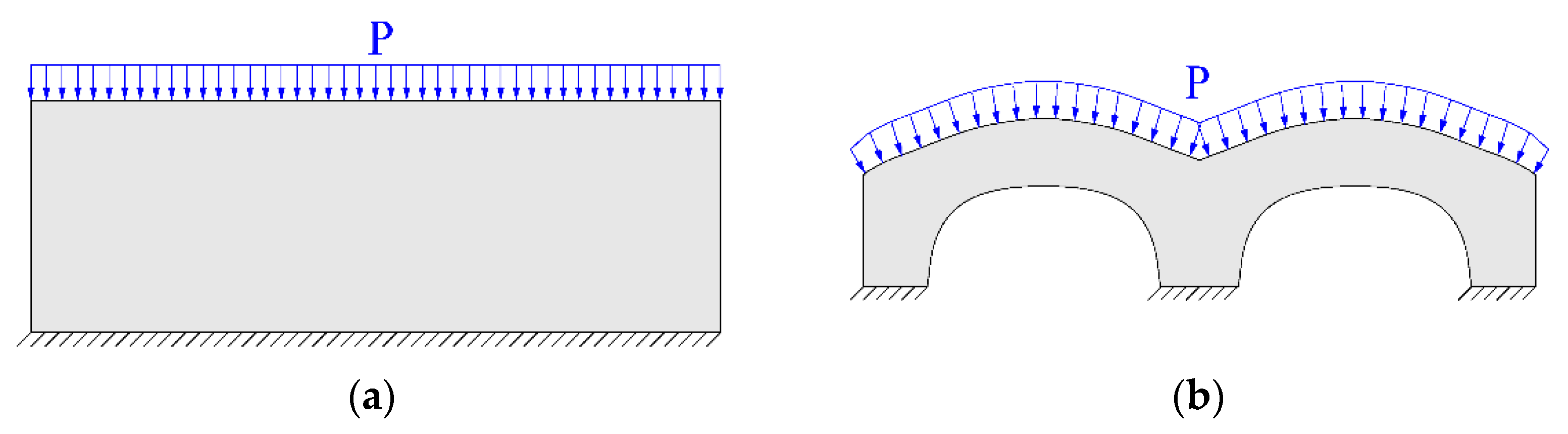
2. Minimum Compliance Design Problem of the Structures with Design-Dependent Loads

When considering the topology optimization problem with design-dependent loads, it means that the positions or directions of the applied loads keep changing with the evolution of the structural topologies. Figure 1 shows a schematic representation of design-dependent loads during the optimization iterations.

The original design is shown in Figure 1a, and a pressure force $P$ is applied on the top of the original structure. As the optimization iterations continue, the original structure changes, and the locations and directions of the applied pressure load $P$ changes accordingly (see Figure 1b).

In this paper, the topology optimization aimed at minimizing the compliance of a structure subjected to design-dependent pressure loads with given material usage, and the formulation is as follows:

$$\begin{array}{l}\mathrm{find} \chi \\ \min C=P{\left(\chi \right)}^{\mathrm{T}}u\left(\chi \right)\\ \mathrm{s}.\mathrm{t}. K\left(\chi \right)u=P\left(\chi \right)\\ {\displaystyle \int \chi }d\Omega \le V^{*}\\ \chi =0\hspace{0.17em}\hspace{0.17em}or\hspace{0.17em}\hspace{0.17em}1\end{array}$$

(1)

where $C$ is the structure mean compliance and the 0/1 discrete function $\chi$ denotes the structural topology, i.e., $\chi =0$ signifies a void material, while $\chi =1$ signifies a solid material. $K$ is the stiffness matrix. $u$ is the structural nodal displacement vector obtained from the linear or nonlinear equilibrium equation $K\left(\chi \right)u=P\left(\chi \right)$. $V^{*}$ is the constant volume of the material constraint.

3. Topology Optimization Based on Material-Field Series Expansion Model and Adaptive Body-Fitted Mesh

3.1. Bounded Material Field Definition

Here, a bounded material-field function $\phi \left(x\right)\in \left[-1,1\right]$ with a certain degree of correlation behavior was defined in the design domain $x\in {\Omega }_x$ to describe the structural topology $\chi$. The mathematical description of the structural topology with the material-field function was represented as follows:

$$\{\begin{array}{l}\chi =0, \mathrm{if} -1\le \phi \left(x\right)\le d_z\\ \chi =1, \mathrm{if} d_z<\phi \left(x\right)\le 1\end{array}$$

(2)

where $d_z$ is a given threshold which satisfies $-1<d_z\le 0$.

For the material-field function $\phi \left(x\right)$, the spatial correlation at the two points closely depends on their spatial distance, and an exponential model was used to describe the correlation as follows:

$$R\left(x_1,x_2\right)=\exp \left(-\frac{{\Vert x_1-x_2\Vert }^2}{L_c^2}\right)$$

(3)

where $x_1$ and $x_2$ are any two points in the design domain $x\in {\Omega }_x$, and $L_c$ is the correlation length of the material field. According to Equation (3), the correlation length $L_c$ is an important factor for determining the correlation between the two points. Therefore, the correlation length $L_c$ determined the spatial fluctuation degree of the material field. When the structural topology was represented by the material field $\phi \left(x\right)$, the value of the correlation length $L_c$ could be used to control the degree of detail of the structures [24]. For a 2D rectangular design domain with dimensions $l_a$ and $l_b$, the correlation length was set to $L_c=0.3\cdot \min \left(l_a,l_b\right)$ in this study.

3.2. Reduced Series Expansion of the Material Field

Based on the theory of bounded fields [37,38,39], the design domain was discretized into a finite number of regularly arranged material-field observation points $x_i\left(i=1,2,\dots ,N_P\right)$, and the series expansion of the material-field $\phi \left(x\right)$ was expressed by

$$\phi \left(x,\xi \right)={\displaystyle \sum _{j=1}^{N_P}\left(\frac{1}{\sqrt{{\alpha }_j}}{\psi }_j^{\mathrm{T}}{C}_P\left(x\right){\xi }_j\right)}$$

(4)

where $C_P\left(x\right)=\left\{R\left(x,x_1\right) R\left(x,x_2\right) \dots R\left(x,x_{N_P}\right)\right\}$ is a vector, that contains the correlation between $x$ and all the material-field points, and $\xi ={\left\{{\xi }_1 {\xi }_2 \dots {\xi }_{N_P}\right\}}^{\mathrm{T}}$ is a vector of uncorrelated MFSE coefficients. ${\alpha }_j$ and ${\psi }_j$ are the eigenvalues and eigenvectors of the correction matrix $R$, which is expressed as follows:

$$R=\left[\begin{array}{cccc}R\left(x_1,x_1\right)& R\left(x_1,x_2\right)& \cdots & R\left(x_1,x_{N_P}\right)\\ R\left(x_2,x_1\right)& R\left(x_2,x_2\right)& \cdots & R\left(x_2,x_{N_P}\right)\\ ⋮& ⋮& \ddots & ⋮\\ R\left(x_{N_P},x_1\right)& R\left(x_{N_P},x_2\right)& \cdots & R\left(x_{N_P},x_{N_P}\right)\end{array}\right]$$

(5)

The eigenvalues ${\alpha }_j$ of $R$ are in descending order. The greater the eigenvalues, the greater the contribution to the corresponding expansion item in Equation (4). Therefore, considering the question of improving the calculation efficiency without losing sufficient accuracy, it is efficient to truncate Equation (4) to only a few main $M$ items ($M<<N_P$). The truncation criterion is as follows:

$${\displaystyle \sum _{m=1}^M{\alpha }_m}\approx \left(1-\epsilon \right)\cdot {\displaystyle \sum _{m=1}^{N_P}{\alpha }_m}$$

(6)

where $\epsilon$ is a small number. In this paper, we set $\epsilon =0.001$.

After the truncation of Equation (4), the material-field $\phi \left(x\right)$ could be approximately expressed in the vector form, which is

$$\phi \left(x,\xi \right)\approx {\xi }^{\mathrm{T}}{\Lambda }^{-1/2}{\Psi }^{\mathrm{T}}{C}_P\left(x\right)$$

(7)

where $\xi ={\left\{{\xi }_1 {\xi }_2 \dots {\xi }_M\right\}}^{\mathrm{T}}$ contains the $M$ uncertain coefficients. $\Lambda$ is the diagonal matrix that consists of $M$ eigenvalues ${\alpha }_j$, and $\Psi$ consists of $M$ eigenvectors ${\psi }_j$.

According to the range of the material-field $\phi \left(x,\xi \right)\in \left[-1,1\right]$ and Equation (7), we could obtain

$$-1\le {\xi }^{\mathrm{T}}{\Lambda }^{-1/2}{\Psi }^{\mathrm{T}}{C}_P\left(x_i\right)\le 1,i=1,2,\dots ,N_p$$

(8)

By squaring the Equation (8), we get

$${\xi }^{\mathrm{T}}{\Lambda }^{-1/2}{\Psi }^{\mathrm{T}}{C}_P\left(x_i\right)C_P{\left(x_i\right)}^{\mathrm{T}}\Psi {\Lambda }^{-1/2}\xi \le 1,i=1,2,\dots ,N_p$$

(9)

By introducing the matrix $W_i={\Lambda }^{-1/2}{\Psi }^{\mathrm{T}}{C}_P\left(x_i\right)C_P{\left(x_i\right)}^{\mathrm{T}}\Psi {\Lambda }^{-1/2}$, Equation (8) could be expressed as follows:

$${\xi }^{\mathrm{T}}{W}_i\xi \le 1,\hspace{0.17em} i=1,2,\dots ,N_p$$

(10)

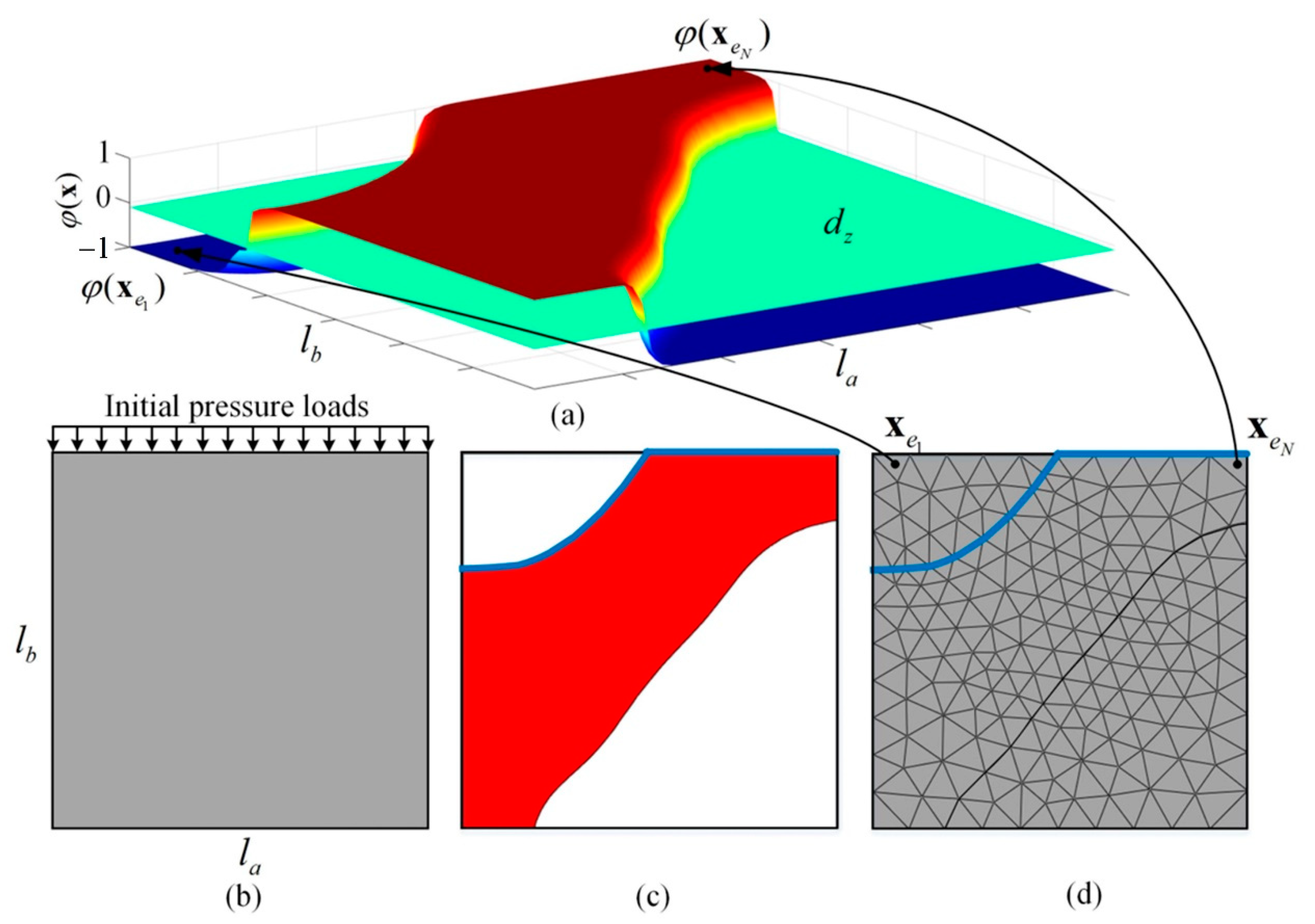
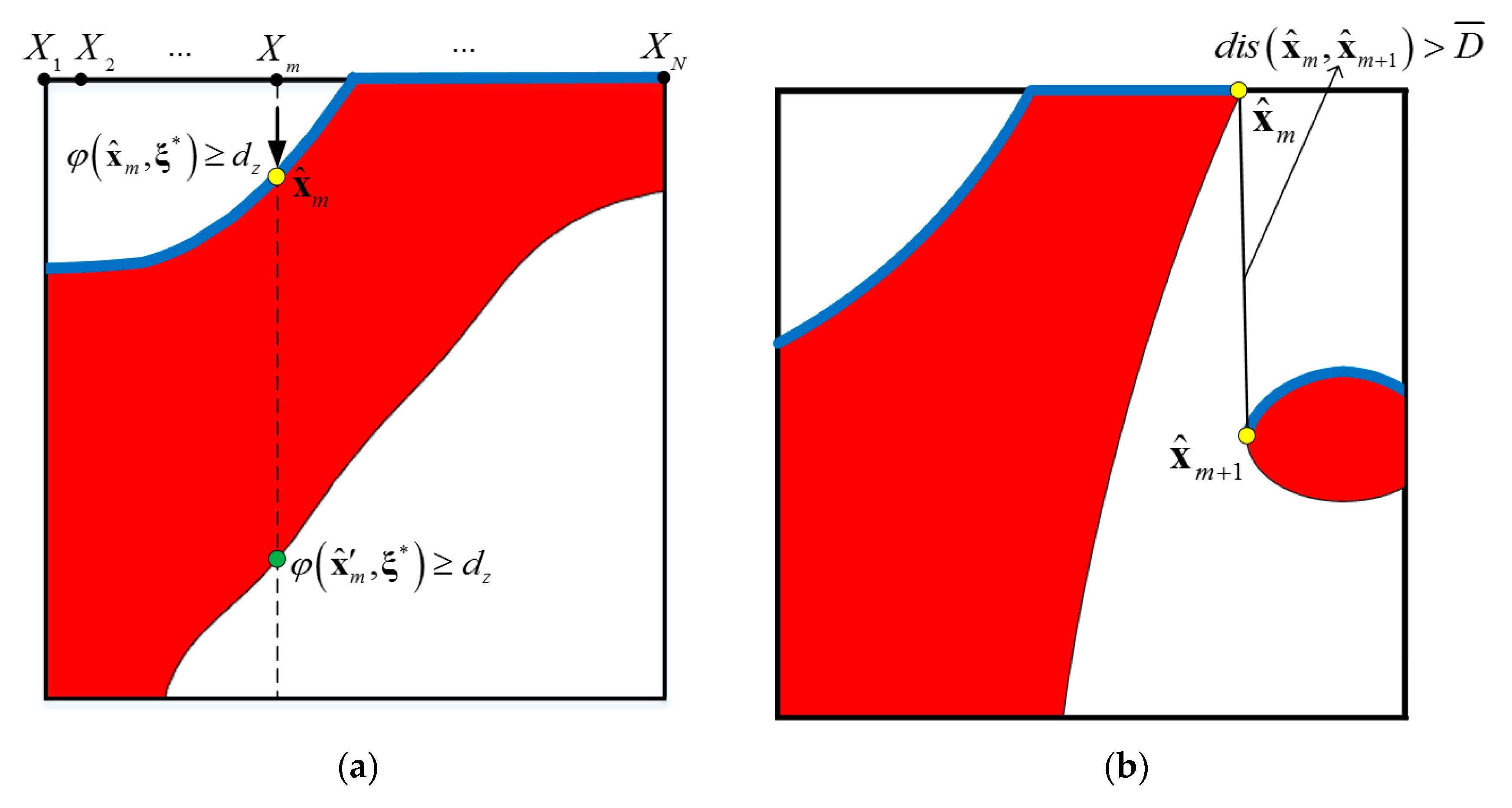
3.3. Identification of the Loading Surface

For topology optimization problems with design-dependent loads, identifying the loading surface is one of the major tasks. In the MFSE method, it is very convenient to identify the loading surface as

$$\{\begin{array}{l}\mathrm{non}-\mathrm{load}-\mathrm{carrying} \mathrm{parts}, \mathrm{if} -1\le \phi \left(x,\xi \right)\le d_z\\ \mathrm{load}-\mathrm{carrying} \mathrm{parts}, \mathrm{if} d_z<\phi \left(x,\xi \right)\le 1\end{array}$$

(11)

where the non-load-carrying parts represent the void material, and the load-carrying parts represent the solid material. In the boundary and topology description of Equation (11), the different realizations of the bounded material field $\phi \left(x,\xi \right)$ and different thresholds $d_z$ represent different loading surfaces. In this study, the value of the threshold $d_z$ is not a fixed value and the maximum value of $d_z$ is 0. The minimum value of $d_z$ depends on the volume constraint $V^{*}$ in the optimization formula Equation (1). Generally speaking, the smaller the volume constraint $V^{*}$, the smaller the minimum value of $d_z$. The value of $d_z$ gradually increased with the optimization process.

The schematic diagram for the loading surface and the body-fitted mesh based on the MFSE is shown in Figure 2. As shown in Figure 2a, we assumed that the design domain is rectangular with a dimension of $l_a\times l_b$. Initial pressure forces were applied on the top edge of the design domain, as shown in Figure 2b and the final loading surface is illustrated in Figure 2c. The whole process mainly consists of three steps as follows:

Step 1:

Represent the Material-Field Function Using Series Expansion

Suppose that there are $N_P$ observation points evenly distributed in the rectangular design domain $x\in {\Omega }_x$ and that the position of the material-field point is represented by $x_1,x_2,\dots ,x_{N_P}$. According to the correlation formulation in Equation (3), the correction matrix $R$ containing the correlation information of all the material-field points can be determined. When a set of uncorrelated MFSE coefficients (design variables) ${\xi }^{*}={\left\{{\xi }_1{}^{*} {\xi }_2{}^{*} \dots {\xi }_M{}^{*}\right\}}^{\mathrm{T}}$ is given, the material-field function value $\phi \left(x,{\xi }^{*}\right)$ in the design domain could be determined using Equation (7). In Figure 2a, a material-field function $\phi \left(x,{\xi }^{*}\right)$ was given, where its upper and lower boundaries are between −1 and 1. The green plate is the given threshold $d_z$, and it was used to cut the material-field function $\phi \left(x,{\xi }^{*}\right)$ and divide the design domain into load-carrying parts and non-load-carrying parts according to Equation (11).

Step 2:

Determine the Load-Carrying Parts and Update the Loading Surface

After cutting the material-field function $\phi \left(x,{\xi }^{*}\right)$ using the given threshold $d_z$, the contours of the function value $\phi \left(x,{\xi }^{*}\right)$ in the design domain are obtained. For the case $\phi \left(x,{\xi }^{*}\right)\ge d_z$, the load-carrying parts are denoted by the red part. The white part in Figure 2c represents the non-load-carrying part that satisfies $\phi \left(x,{\xi }^{*}\right)<d_z$. There is no doubt that the loads were applied to the load-carrying parts. The detailed process of updating the loading surfaces of any structure: (i) When the initial pressure is initially applied on the front edge of the design domain (e.g., Figure 2b), we choose $N$ discrete points $X_m\left(m=1,2,\dots ,N\right)$ uniformly distributed on the initial loading surface as shown in Figure 3a, and we define the distance between adjacent discrete points $X_m$ and $X_{m+1}$ is $\overline{d}$. (ii) Judging the material-field value from each point $X_m$ along the pressure direction and searching out the position ${\widehat{x}}_m$ that first satisfies $\phi \left({\widehat{x}}_m,{\xi }^{*}\right)\ge d_z$ (represented by the yellow dots in Figure 3a). It should be pointed out that if $\phi \left({\widehat{x}}_m,{\xi }^{*}\right)\ge d_z$ does not exist in the design domain, the loading point ${\widehat{x}}_m$ is marked in the back edge of the design domain. (iii) Connecting all the points ${\widehat{x}}_m$ to spline curves which are obtained by the cubic spline interpolation. Based on the above process, the blue curves in Figure 3 for two typical cases are identified as the loading surfaces.

During the proposed gradient-free optimization process, the sample is considered invalid if the loading surface is discontinuous as shown in Figure 3b. These invalid samples are easily identified by judging whether the distance $dis\left({\widehat{x}}_m,{\widehat{x}}_{m+1}\right)$ between two adjacent discrete points ${\widehat{x}}_m$ and ${\widehat{x}}_{m+1}$ on the loading surface is greater than a given value $\overline{D}=5\cdot \overline{d}$.

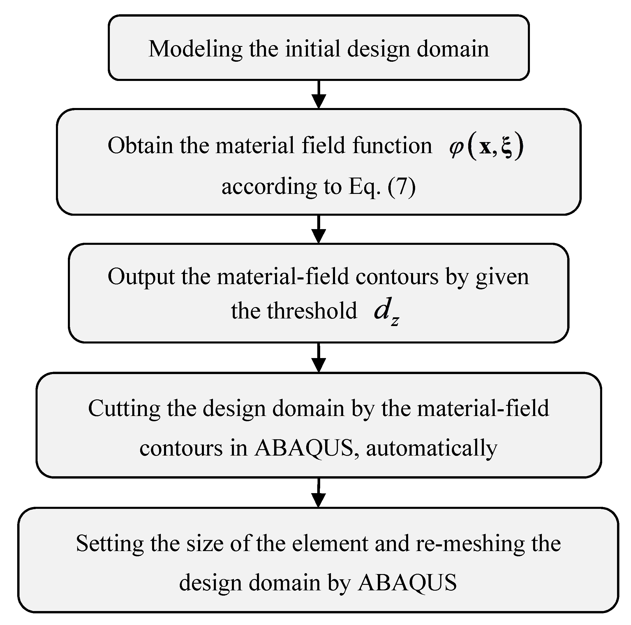
Step 3:

Apply the Pressure Loads and Re-Meshing for the Finite Element Analysis

According to the contour obtained in Step 2, the design domain was cut into several parts: load-carrying parts and non-load-carrying parts. To avoid mesh generation failure for the cutting design domain, it was reasonable to mesh with irregular triangle elements, and the process of meshing is shown in Figure 4. The pressure loads were then applied to the nodes of the triangular elements on the loading surface, as shown in Figure 2d. Suppose that there were $e_N$ triangle elements ($e_1,\dots ,e_N$) in the design domain and that the barycenter of the triangle elements is represented by ($x_{e_1},\dots ,x_{e_N}$), as shown in Figure 2d by the black points. According to the mapping of the material-field function value $\phi \left(x,{\xi }^{*}\right)$, we could determine the material-field function value $\phi \left(x_{e_1},{\xi }^{*}\right),\dots ,\phi \left(x_{e_N},{\xi }^{*}\right)$ at the elemental barycenter $x_{e_1},\dots ,x_{e_N}$. Then, based on the material interpolation function, the material property of each element in Figure 2d was determined to complete the finite element analysis.

3.4. Topology Optimization Formulation for the Structures with Design-Dependent Boundary Loads

According to Equation (2) and the material-field function $\phi \left(x,\xi \right)\in [-1,1]$, it is reasonable to use the SIMP interpolation function to map the material-field function $\phi \left(x,\xi \right)$ to the elastic modulus of the structure. Here, we assumed that there were $e_N$ finite elements, and the interpolation function of the elemental elastic modulus was shown as follows:

$$E_e=E_{\min }+{\left(\frac{1+\tilde{\phi }\left(x_e,\xi \right)}{2}\right)}^3\left(E_0-E_{\min }\right),e=1,2,\dots ,e_N$$

(12)

where $E_0$ is the elastic modulus of fully solid materials, $E_{\min }$ is a small positive value to avoid singularity, and it was assumed that $E_{\min }={10}^{-6}{E}_0$. $\tilde{\phi }\left(x,\xi \right)$ is the Heaviside function projection [40] of the material-field function $\phi \left(x,\xi \right)$, which was used to obtain a clear topology structure, where the function is

$$\tilde{\phi }\left(x_e,\xi \right)=\{\begin{array}{l}\phi \left(x_e,\xi \right)\cdot e^{-\beta }+1-e^{-\beta \cdot \phi \left(x_e,\xi \right)}, \mathrm{if} \phi \left(x_e,\xi \right)\ge 0\\ \phi \left(x_e,\xi \right)\cdot e^{-\beta }-1+e^{-\beta \cdot \phi \left(x_e,\xi \right)}, \mathrm{if} \phi \left(x_e,\xi \right)<0\end{array}$$

(13)

where $\beta$ denotes the smoothing parameter.

According to Equation (7), the minimum compliance topology optimization problem using the MFSE method was expressed as follows:

$$\begin{array}{l}\mathrm{find} \xi \\ \min C=P{\left(\xi \right)}^{\mathrm{T}}u\left(\xi \right)\\ \mathrm{s}.\mathrm{t}. K\left(\xi \right)u\left(\xi \right)=P\left(\xi \right)\\ {\displaystyle \sum _{e=1}^{e_N}{\rho }_e\left(\xi \right)V_e\le V^{*}}\\ {\xi }^{\mathrm{T}}{W}_e\xi \le 1,\hspace{0.17em}e=1,2,\dots ,e_N\end{array}$$

(14)

where $V_e$ denotes the eth elemental volume, and the design variables are the MFSE coefficients $\xi ={\left\{{\xi }_1,{\xi }_2,\dots ,{\xi }_M\right\}}^{\mathrm{T}}$ in the $\xi$-space. Note that the elemental relative density could be determined using ${\rho }_e\left(\xi \right)=\frac{1+\tilde{\phi }\left(x_e,\xi \right)}{2}$.

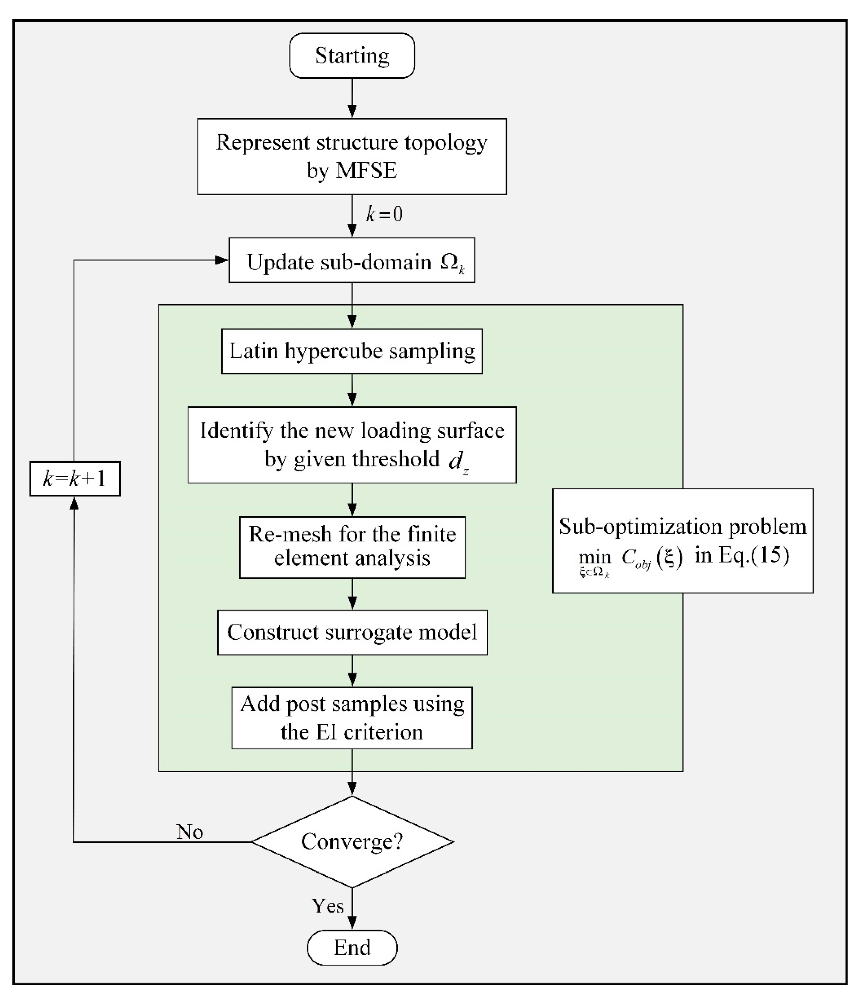
4. Sequential Kriging-Based Optimization Algorithm

In this study, we used the sequential optimization algorithm [24] based on the Kriging surrogate model to complete the MFSE-based topology optimization problem (15) with design-dependent loads. According to the algorithm, in each sub-domain ${\Omega }_k$, the topology optimization model in Equation (14) needs to be converted to the unconstrained form, which is:

$$\min C_{obj}=P{\left(\xi \right)}^{\mathrm{T}}u\left(\xi \right)+p_0\cdot \max \left(\underset{i}{\max }\left(\left({\displaystyle \sum _{e=1}^{e_N}{\rho }_e\left(\xi \right)V_e-V^{*}}\right),\left({\xi }^{\mathrm{T}}{W}_e\xi -1\right)\right),0\right)$$

(15)

where $p_0$ is the penalty multiplier.

The sequential Kriging-based optimization algorithm consists of several sub-optimization problems, where each sub-optimization problem contains two steps: (i) choosing initial samples using Latin hypercube sampling to construct a surrogate model [41]; (ii) adding post samples using the EI criterion to obtain a smaller objective function value. The number of the post sampling $N_s$ is 30 in this paper.

To improve the accuracy of the surrogate model and the searching efficiency as well as reduce the number of invalid loading surfaces during sampling, it is necessary to use the self-adaptive strategy of adjusting the design domain to deal with the topology optimization problem with design-dependent pressure loads in the Kriging-based algorithm. For the specific implementation processes of the self-adaptive strategy, see literature [24]. In this paper, the structural samples of the invalid loading surface will produce poor performance, and it should be pointed out that the Kriging-based optimization algorithm can effectively avoid the omission of the invalid loading surface (judged by $dis\left({\widehat{x}}_m,{\widehat{x}}_{m+1}\right)>\overline{D}$) in Section 3.3.

The flow chart of gradient-free topology optimization with design-dependent boundary loads is illustrated in Figure 5. The convergence criterion of the optimization procedure is that the change of the objective function in two consecutive iterations is less than 0.01.

5. Numerical Examples

To validate the effectiveness of the proposed method for the topology optimization with design-dependent pressure loads, we here presented five examples, including an example with contact supports with friction. In each example, Young’s modulus and Poisson’s ratio of the material were $E_0=200 \mathrm{GPa}$, and $\upsilon =0.3$, respectively. The initial value of the smoothing parameter $\beta$ was zero, and it was gradually increased to 20 during the optimization process. The plane stress assumption was considered for all the examples. The finite element re-meshing and analysis were completed in the commercial package ABAQUS. The number of design variables in Equation (14) is 38 for examples 1, 2, and 3, 53 for example 4, and 63 for example 5.

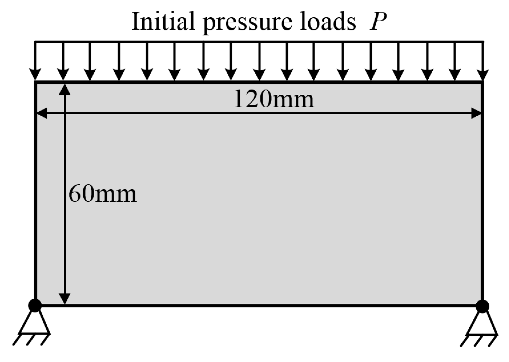
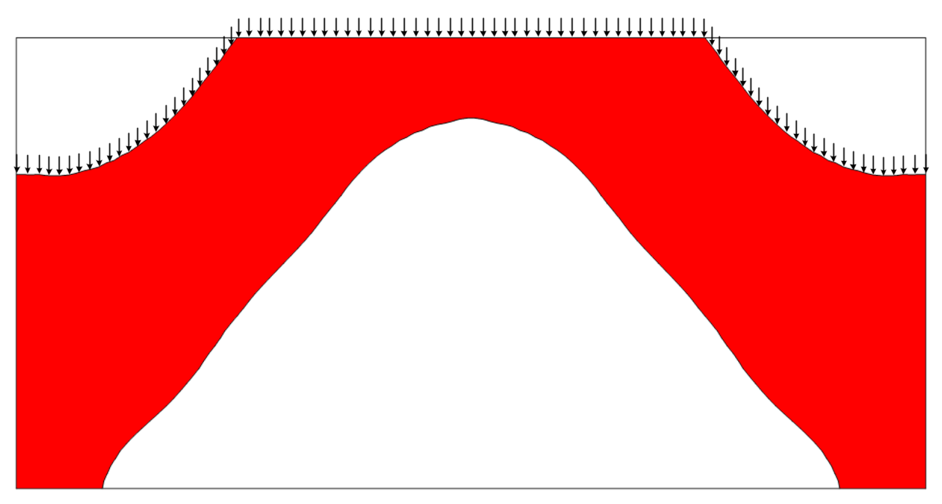
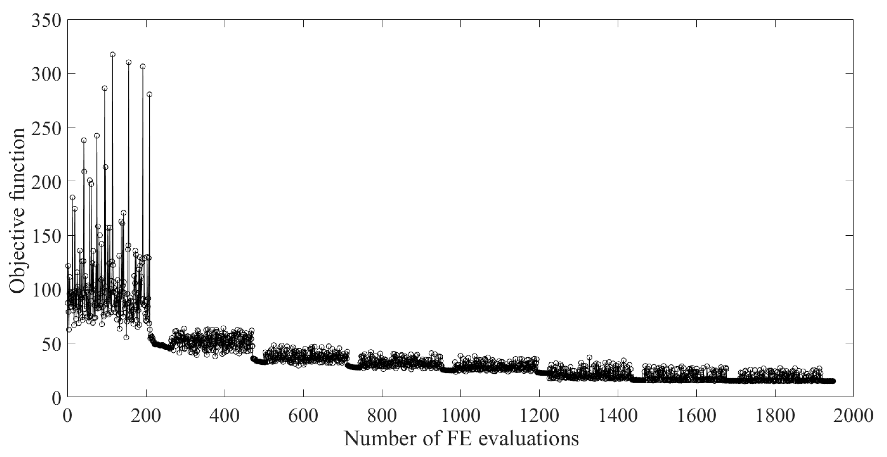
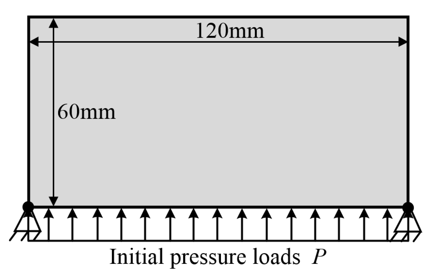
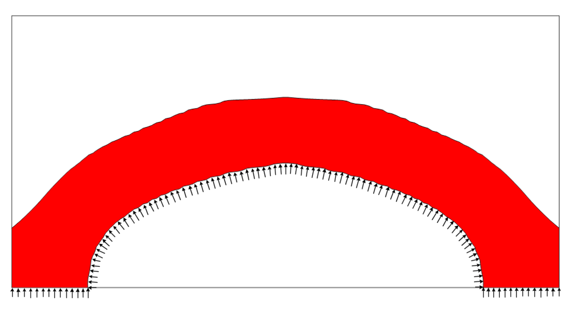
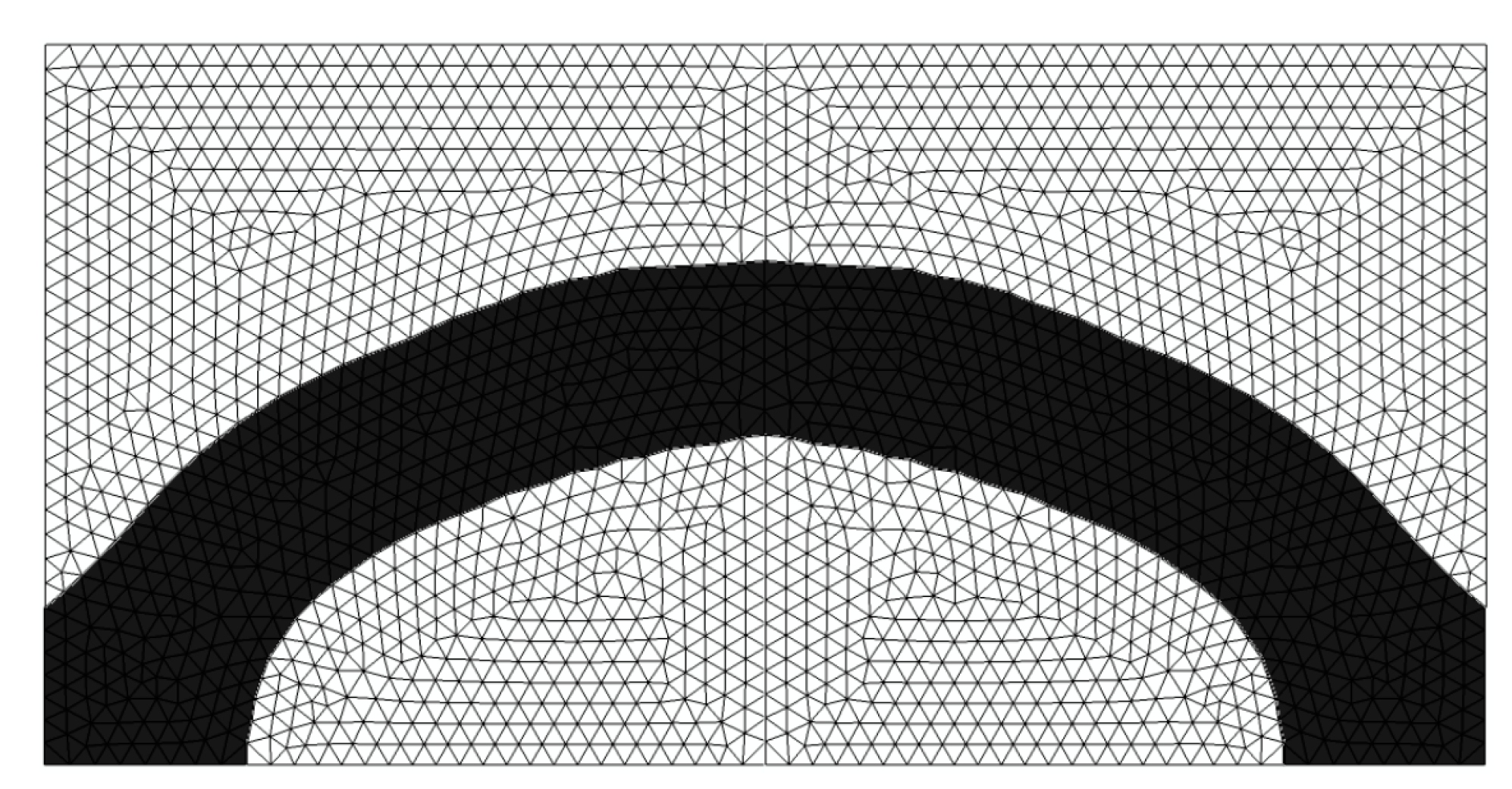
5.1. Example 1

In this example, a bridge-like rectangular structure with sides $l_x=120 \mathrm{mm}$ and $l_y=60 \mathrm{mm}$ was considered, as shown in Figure 6. The structure was clamped at the two bottom corners and subjected to an initial pressure $P=10 \mathrm{N}/\mathrm{mm}$ from its top edge. The directions of the pressure loads were fixed, and the allowable material volume fraction was 50%.

The optimized design is shown in Figure 7 and its compliance is $C=118.29\mathrm{Nmm}$. In Figure 7, the red part is the load-carrying part, where the new loading surface remained on the top edge of the load-carrying part. After cutting the design domain with the contour, we meshed the design domain with the triangle element shown in Figure 8. Based on the interpolation function in Equation (11), the elemental relative density in Figure 8 could be obtained. Figure 9 shows the optimized solution for the bridge-like structure example obtained with a gradient-based method by Du [9]. Compare the optimized topology in Figure 7 and Figure 9, it can be seen that these two results are very similar. The two optimized solutions consist of a global single arch without small columns, and the curvature center of the loading surface is located above the top surface of the structure. In addition, for the optimal solution of reference [9] (Figure 9), the same load and boundary conditions as in Example 1 are applied to the structure, and the compliance of the structure is $C=118.82 \mathrm{Nmm}$, which is almost the same as the compliance of the optimal structure in this paper ($C=118.82 \mathrm{Nmm}$ vs. $C=118.29 \mathrm{Nmm}$).

The iteration history of the proposed MFSE-based gradient-free method with adaptive body-fitted meshes for solving the topology optimization problem with design-dependent loads was plotted in Figure 10. The objective function converged to a stable value during the iteration process while adjusting the design domain. The reason for the appearance of the fluctuant objective function is due to the Latin hypercube sampling in each sub-optimization.

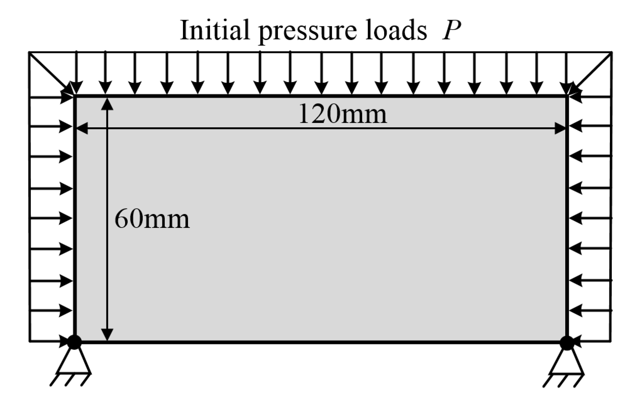
5.2. Example 2

In this example, the optimization of a cover-like structure with the directions of the pressure loads perpendicular to the loading surface was considered. Figure 11 shows the design domain, boundary conditions, and initial pressure loads $P=10 \mathrm{N}/\mathrm{mm}$. The sides of the rectangular design domain are $l_x=120 \mathrm{mm}$ and $l_y=60 \mathrm{mm}$, and the allowable material volume fraction is 30%.

The optimized topology for the cover-like structure is shown in Figure 12, and the final objective function is $C=132.68 \mathrm{Nmm}$. The elemental relative density of the triangle element in the design domain is shown in Figure 13. As seen in Figure 12, the optimized topology for the cover-like structure is an arched structure, which is similar to the optimized solution obtained by Zhang [12] and Neofytou [23]. Therefore, it can be seen that the proposed method is effective in solving the topology optimization problem with design-dependent loads.

5.3. Example 3

The design domain and boundary conditions of the structure in this example are similar to those in Section 5.1, while the position and directions of the initial pressure loads are different. As shown in Figure 14, the bridge-like structure was subjected to constant initial pressure loads $P=10 \mathrm{N}/\mathrm{mm}$ on the top, left, and right edges and the pressure load direction was perpendicular to the loading surface. The final volume fraction was set to 50%.

The bridge-like structure optimum solution and the elemental relative density of the design domain are shown in Figure 15 and Figure 16, and the final compliance of this optimum topology is $C=160.88 \mathrm{Nmm}$. As seen in Figure 15, the curvature center of the curved loading surface is below the structure. As the spherical shape is theoretically an ideal structure for a pressure vessel, this optimized structure is also intuitively the expected solution.

5.4. Example 4

This piston head structure was introduced in literature [21], as shown in Figure 17. The design domain is a rectangle whose size $120 \mathrm{mm}\times 40 \mathrm{mm}$, and it was subjected to an initial pressure of $P=10 \mathrm{N}/\mathrm{mm}$ applied on its top edge. The direction of the pressure loads was perpendicular to the loading surface. In Figure 17, the degrees of freedom along the horizontal direction are constrained on the left and right sides, and the central point of the bottom edge of the structure is fully constrained. A volume fraction of 40% was applied.

Figure 18 shows the structural topology of piston head structure subjected to design-dependent loads by using the proposed method, where the compliance value of this optimized design is $C=160.99 \mathrm{Nmm}$. As shown in Figure 18, from an overall look, the gradient-free optimized solution in this study is similar to the design from Emmendoerfer et al. [21]. In addition, the triangle element grid of the design domain and the elemental relative density are shown in Figure 19.

5.5. Example 5

The last example considered a two-point supported beam structure, whose sides were $120 \mathrm{mm}\times 30 \mathrm{mm}$, where the friction contact effect and geometrical nonlinearity were considered. Generally speaking, for large deformation contact problems, the contact position of a structure changes when a load is applied. Therefore, to ensure the consistency of the structure in the initial position, we added a non-design domain part, whose sides were $120 \mathrm{mm}\times 1 \mathrm{mm}$, at the bottom of the structure, as shown in Figure 20. The beam was placed on two semi-circular supports with a radius of $r=30 \mathrm{mm}$. Both supports were rigid and had a friction coefficient of $f_c=0.15$ with the surface of the beam. An initial pressure $P$ was applied at the top edge of the structure, and the directions of the pressure loads were fixed. The allowable material volume fraction was 50%.

The optimized solutions for the structure subjected to different values of pressure loads, $P=10 \mathrm{N}/\mathrm{mm}$ and $P=3.2 \mathrm{KN}/\mathrm{mm}$, are presented in Figure 21a,b, respectively. As seen in Figure 21, the two optimized topologies for the cases with the two loads have distinct differences. The length of the solid material at the bottom of the beam structure in Figure 21a is significantly greater than that of the structure in Figure 21b. The reason for this is that with the increase in the pressure load, the contact point between the beam and the two semi-circular supports changes inwards.

The deformed configurations of the optimal solutions in Figure 21 for the two cases are shown in Figure 22a,b. The deformation of the structure for $P=3.2 \mathrm{KN}/\mathrm{mm}$ was significantly greater than that of the structure for $P=10 \mathrm{N}/\mathrm{mm}$ ($u_{\max }=3.38 \mathrm{mm}$ vs. $u_{\max }=0.027 \mathrm{mm}$). This means that for the topology optimization with design-dependent loads, the large pressure loads have an important influence on the optimal material layout. Here, it should be noted that for the geometrical nonlinearity and contact problems considering the friction coefficient, it would be difficult to analytically derive the sensitivity of the objective function. According to the optimized solutions in Figure 21, this reveals that it is also effective to implement the gradient-free method to deal with the complex topology optimization problem with design-dependent loads.

6. Conclusions

In this paper, an effective gradient-free topology optimization strategy is adopted to deal with continuum structures subjected to design-dependent loads. Based on the MFSE model, it is convenient to generate a body-fitted finite element mesh and to identify the loading surface for the application of the design-dependent boundary loads. Furthermore, the design variables used to describe the structure topology are significantly reduced. The topology optimization problem is solved by using the sequential Kriging-based optimization algorithm with a self-adaptive design space adjusting strategy. Numerical examples show the validity and effectiveness of the proposed method.

Although more than 2000 finite element analyses are required to complete the proposed gradient-free topology optimization, it will have developing prospect in practical engineering since the proposed method does not need sensitivity information. With the rapid development of computer hardware and parallel processing technology, the computational costs of the proposed method will not be a heavy burden shortly. It can be easily implemented to solve complex nonlinear problems considering design-dependent loads, contact effects, and geometrical nonlinearity.

References

- Bendsøe, M.P.; Kikuchi, N. Generating optimal topologies in structural design using a homogenization method. Comput. Methods Appl. Mech. Eng. 1988, 71, 197–224. [Google Scholar] [CrossRef]
- Eschenauer, H.A.; Olhoff, N. Topology optimization of continuum structures: A review. Appl. Mech. Rev. 2001, 54, 1453–1457. [Google Scholar] [CrossRef]
- Bendsøe, M.P.; Sigmund, O. Topology Optimization: Theory, Methods and Applications, 2nd ed.; Springer: Berlin/Heidelberg, Germany; New York, NY, USA, 2003. [Google Scholar]
- Allaire, G.; Jouve, F.; Toader, A. Structural optimization using sensitivity analysis and a level-set method. J. Comput. Phys. 2004, 194, 363–393. [Google Scholar] [CrossRef] [Green Version]
- Wang, X.; Wang, M.Y.; Guo, D. Structural shape and topology optimization in a level-set-based framework of region representation. Struct. Multidiscip. Optim. 2004, 27, 1–19. [Google Scholar] [CrossRef]
- Sigmund, O.; Maute, K. Topology optimization approaches. Struct. Multidiscip. Optim. 2013, 48, 1031–1055. [Google Scholar] [CrossRef]
- Deaton, J.D.; Grandhi, R.V. A survey of structural and multidisciplinary continuum topology optimization: Post 2000. Struct. Multidiscip. Optim. 2014, 49, 1–38. [Google Scholar] [CrossRef]
- Hammer, V.B.; Olhoff, N. Topology optimization of continuum structures subjected to pressure loading. Struct. Multidiscip. Optim. 2000, 19, 85–92. [Google Scholar] [CrossRef]
- Du, J.; Olhoff, N. Topological optimization of continuum structures with design-dependent surface loading–Part I: New computational approach for 2D problems. Struct. Multidiscip. Optim. 2004, 27, 151–165. [Google Scholar] [CrossRef]
- Fuchs, M.B.; Shemesh, N. Density-based topological design of structures subjected to water pressure using a parametric loading surface. Struct. Multidiscip. Optim. 2004, 28, 11–19. [Google Scholar] [CrossRef]
- Zhang, H.; Zhang, X.; Liu, S. A new boundary search scheme for topology optimization of continuum structures with design dependent loads. Struct. Multidiscip. Optim. 2008, 37, 121–129. [Google Scholar] [CrossRef]
- Chen, B.; Kikuchi, N. Topology optimization with design-dependent loads. Finite Elem. Anal. Des. 2001, 37, 57–70. [Google Scholar] [CrossRef]
- Bourdin, B.; Chambolle, A. Design-dependent loads in topology optimization. ESAIM Control Optim. Calc. Var. 2003, 9, 19–48. [Google Scholar] [CrossRef]
- Sigmund, O.; Clausen, P.M. Topology optimization using a mixed formulation: An alternative way to solve pressure load problems. Comput. Methods Appl. Mech. Eng. 2007, 196, 1874–1889. [Google Scholar] [CrossRef] [Green Version]
- Yoon, G.H.; Jensen, J.S.; Sigmund, O. Topology optimization of acoustic-structure problems using a mixed finite element formulation. Int. J. Numer. Methods Eng. 2007, 70, 1049–1075. [Google Scholar] [CrossRef]
- Yoon, G.H. Topology optimization for stationary fluid-structure interaction problems using a new monolithic formulation. Int. J. Numer. Methods Eng. 2010, 82, 591–616. [Google Scholar] [CrossRef]
- Lundgaard, C.; Alexandersen, J.; Zhou, M.; Andreasen, C.; Sigmund, O. Revisiting density-based topology optimization for fluid-structure-interaction problems. Struct. Multidiscip. Optim. 2018, 58, 969–995. [Google Scholar] [CrossRef] [Green Version]
- Yang, X.Y.; Xie, Y.M.; Steven, G.P. Evolutionary methods for topology optimisation of continuous structures with design dependent loads. Comput. Struct. 2005, 83, 956–963. [Google Scholar] [CrossRef]
- Xia, Q.; Wang, M.Y.; Shi, T. Topology optimization with pressure load through a level set method. Comput. Methods Appl. Mech. Eng. 2015, 283, 177–195. [Google Scholar] [CrossRef]
- Shu, L.; Wang, M.Y.; Ma, Z. Level set based topology optimization of vibrating structures for coupled acoustic-structural dynamics. Comput. Struct. 2014, 132, 34–42. [Google Scholar] [CrossRef]
- Emmendoerfer, H.; Fancello, E.; Silva, E. Level set topology optimization for design-dependent pressure load problems. Int. J. Numer. Methods Eng. 2018, 115, 825–848. [Google Scholar] [CrossRef]
- Picelli, R.; Neofytou, A.; Kim, H.A. Topology optimization for design-dependent hydrostatic pressure loading via the level-set method. Struct. Multidiscip. Optim. 2019, 60, 1313–1326. [Google Scholar] [CrossRef] [Green Version]
- Neofytou, A.; Picelli, R.; Huang, T.H.; Chen, J.S.; Kim, H.A. Level set topology optimization for design-dependent pressure loads using the reproducing kernel particle method. Struct. Multidiscip. Optim. 2020, 61, 1805–1820. [Google Scholar] [CrossRef]
- Lohan, D.J.; Dede, E.M.; Allison, J.T. Topology optimization for heat conduction using generative design algorithms. Struct. Multidiscip. Optim. 2015, 55, 1063–1077. [Google Scholar] [CrossRef]
- Yoshimura, M.; Shimoyama, K.; Misaka, T.; Obayashi, S. Topology optimization of fluid problems using genetic algorithm assisted by the Kriging model. Int. J. Numer. Methods Eng. 2016, 109, 514–532. [Google Scholar] [CrossRef] [Green Version]
- Raponi, E.; Bujny, M.; Olhofer, M.; Aulig, N.; Boria, S.; Duddeck, F. Kriging-assisted topology optimization of crash structures. Comput. Methods Appl. Mech. Eng. 2019, 348, 730–752. [Google Scholar] [CrossRef]
- Vimal, J.; Savsani, V.J.; Patel, V.K. Truss topology optimization with static and dynamic constraints using modified subpopulation teaching–learning-based optimization. Eng. Optim. 2016, 48, 1990–2006. [Google Scholar]
- Tejani, G.; Savsani, V. Teaching-learning-based optimization (TLBO) approach to truss structure subjected to static and dynamic constraints. In Proceedings of International Conference on ICT for Sustainable Development; Springer: Singapore, 2016; pp. 63–71. [Google Scholar]
- Tejani, G.G.; Savsani, V.J.; Patel, V.K. Modified sub-population teaching-learning-based optimization for design of truss structures with natural frequency constraints. Mech. Based Des. Struct. Mach. 2016, 44, 495–513. [Google Scholar] [CrossRef]
- Yan, Y.; Liu, P.; Zhang, X.; Luo, Y. Photonic crystal topological design for polarized and polarization-independent band gaps by gradient-free topology optimization. Opt. Express 2021, 29, 24861–24883. [Google Scholar] [CrossRef]
- Zhang, X.; Luo, Y.; Yan, Y.; Liu, P.; Kang, Z. Photonic band gap material topological design at specified target frequency. Adv. Theory Simul. 2021, 4, 2100125. [Google Scholar] [CrossRef]
- Liu, P.; Zhang, X.; Luo, Y. Topological Design of Freely Vibrating Bi-Material Structures to Achieve the Maximum Band Gap Centering at a Specified Frequency. J. Appl. Mech. 2021, 88, 081003. [Google Scholar] [CrossRef]
- Liu, P.; Yan, Y.; Zhang, X.; Luo, Y.; Kang, Z. Topological design of microstructures using periodic material-field series-expansion and gradient-free optimization algorithm. Mater. Des. 2021, 199, 109437. [Google Scholar] [CrossRef]
- Zhang, X.; Xing, J.; Liu, P.; Luo, Y.; Kang, Z. Realization of full and directional band gap design by non-gradient topology optimization in acoustic metamaterials. Extrem. Mech. Lett. 2021, 42, 101126. [Google Scholar] [CrossRef]
- Zhang, X.; Li, Y.; Wang, Y.; Jia, Z.; Luo, Y. Narrow-band filter design of phononic crystals with periodic point defects via topology optimization. Int. J. Mech. Sci. 2021, 212, 106829. [Google Scholar] [CrossRef]
- Liu, P.; Yan, Y.; Zhang, X.; Luo, Y. A MATLAB code for the material-field series-expansion topology optimization method. Front. Mech. Eng. 2021, 16, 607–622. [Google Scholar] [CrossRef]
- Luo, Y.; Xing, J.; Kang, Z. Topology optimization using material-field series expansion and Kriging-based algorithm: An effective non-gradient method. Comput. Methods Appl. Mech. Eng. 2020, 364, 112966. [Google Scholar] [CrossRef]
- Luo, Y.; Zhan, J.; Xing, J.; Kang, Z. Non-probabilistic uncertainty quantification and response analysis of structures with a bounded field model. Comput. Methods Appl. Mech. Eng. 2019, 347, 663–678. [Google Scholar] [CrossRef]
- Luo, Y.; Bao, J. A material-field series-expansion method for topology optimization of continuum structures. Comput. Struct. 2019, 225, 106122. [Google Scholar] [CrossRef]
- Wang, F.; Lazarov, B.S.; Sigmund, O. On projection methods, convergence and robust formulations in topology optimization. Struct. Multidiscip. Optim. 2011, 43, 767–784. [Google Scholar] [CrossRef]
- Joseph, R.V.; Hung, Y. Orthogonal-maximin Latin hypercube designs. Stat. Sin. 2012, 18, 171–186. [Google Scholar]
Publisher’s Note: MDPI stays neutral with regard to jurisdictional claims in published maps and institutional affiliations. |
© 2021 by the authors. Licensee MDPI, Basel, Switzerland. This article is an open access article distributed under the terms and conditions of the Creative Commons Attribution (CC BY) license (https://creativecommons.org/licenses/by/4.0/).
Share and Cite
Zhan, J.; Li, J.; Liu, P.; Luo, Y. A Gradient-Free Topology Optimization Strategy for Continuum Structures with Design-Dependent Boundary Loads. Symmetry 2021, 13, 1976. https://doi.org/10.3390/sym13111976
Zhan J, Li J, Liu P, Luo Y. A Gradient-Free Topology Optimization Strategy for Continuum Structures with Design-Dependent Boundary Loads. Symmetry. 2021; 13(11):1976. https://doi.org/10.3390/sym13111976
Chicago/Turabian StyleZhan, Junjie, Jing Li, Pai Liu, and Yangjun Luo. 2021. "A Gradient-Free Topology Optimization Strategy for Continuum Structures with Design-Dependent Boundary Loads" Symmetry 13, no. 11: 1976. https://doi.org/10.3390/sym13111976
APA StyleZhan, J., Li, J., Liu, P., & Luo, Y. (2021). A Gradient-Free Topology Optimization Strategy for Continuum Structures with Design-Dependent Boundary Loads. Symmetry, 13(11), 1976. https://doi.org/10.3390/sym13111976