A Prabhakar Fractional Approach for the Convection Flow of Casson Fluid across an Oscillating Surface Based on the Generalized Fourier Law

Abstract

In the present work, an unsteady convection flow of Casson fluid, together with an oscillating vertical plate, is examined. The governing PDEs corresponding to velocity and temperature profile are transformed into linear ODEs with the help of the Laplace transform method. The ordinary derivative model generalized to fractional model is based on a generalized Fourier law. The solutions for energy and velocity equations are obtained after making the equations dimensionless. To check the insight of the physical parameters, especially the symmetric behavior of fractional parameters, it is found that for small and large values of time, fluid properties show dual behavior. Since the fractional derivative exhibits the memory of the function at the chosen value of time, therefore the present fractional model is more suitable in exhibiting memory than the classical model. Such results can be useful in the fitting of real data where needed. In the limiting case when fractional parameters are taken $\beta =\gamma$ = 0 and $\alpha$ = 1 for both velocity and temperature, we get the solutions obtained with ordinary derivatives from the existing literature.

1. Introduction

Casson proposed the Casson fluid model in 1959 to predict flow patterns of suspended pigment–oil mixtures. These fluids are known as viscoelastic fluids, and they have a broad range of uses in the drilling process. Honey jelly soup, concentrated fruit juices and artificial fibers are all forms of Casson fluid [1]. The Casson fluid model has many uses in biomechanics and processes. In comparison to previous viscoelastic models, the Casson fluid model is more suitable for studying materials such as blood, chocolate, and other rheological details. At zero shear rate, Casson fluid is a shear-thinning liquid with infinite viscosity. The fluid behaves like a solid when the yield stress is greater than the shear stress [2,3]. Based on generalized Fourier’s and Fick’s laws, as well as mass and heat transfer, new fractional derivative model Casson fluid has been developed by Sheikh et al. [4]. A new method for solving the fractional generalized Casson fluids model of the Caputo fractional operator has been developed by Ndolane [5]. Arif et al. [6] deliberated applications of motor oil using a fractional model of Casson fluids of ramped wall temperature. Ali et al. [7] described Wright’s function solutions for time fractional Casson fluid flow in free convection. Raza et al. [8] conducted thermal movement of conservative Casson nanoparticles through ramped temperature because of an infinite perpendicular plate by fractional derivative. Khan et al. [9] examined Casson fluid fractional derivative generalized unsteady flow because of the infinite plate. Saqib et al. [10] expressed nonlocal fractional model of BTF incorporating hybrid nanoparticles with symmetric MHD channel flow.

Oscillating flow is a well-known reason for higher mass and heat transfer. Oscillating movement was realized moreover by fluids vibration around a fixed article. While fluids vibration around a fixed object needs more energy. Oscillating flows are widely used in piston engines, pulsating burners, heat exchangers, cryogenic refrigeration, chemical reactors, and in numerous applications in the atmosphere military and industry fields [11,12]. Song et al. [13] discussed the significance of exponentially Darcy’s and heating law for second grade fluid flow with oscillating plate by utilizing the Atangana–Baleanu time fractional operator. Ali et al. [14] analyzed the flow of second grade fluids on an oscillating perpendicular plate for unsteady free convection closed arrangement solutions. Haider et al. [15] deliberated heat transfer of micro polar hybrid nanofluids through an oscillating vertical plate of Newtonian heating with thermal radiation. Shah et al. [16] observed thermal analysis of second grade fluids over oscillation perpendicular flat plate by consuming time fractional Caputo–Fabrizio derivatives. The impacts of heat generation and thermal diffusion on magnetohydrodynamics (MHD) nanofluids flow through an oscillating vertical plate with permeable medium, as addressed by Sheikholeslami et al. [17].

It is observed that the numerical model of integer-order derivative, counting the non-linear model, does not work satisfactorily in numerous cases. Fractional calculus has many applications in the field of viscoelasticity, signals processing, electromagnetics, fluid mechanics, and optics. It has been utilized to illustrate the model physical and designing forms that are found by fractional differential conditions. Fang et al. [18] discussed Caputo fractional derivatives along with applications of time-fractional distribution equations through a fast technique for variable-order. Dassios and Baleanu [19] introduced Caputo’s fractional-differential equation for singular linear structure with an optimal solution. Ali et al. [20] described hybrid nanofluids along with constant comparative Caputo fractional derivatives of power laws memory because of a pressure gradient. Baleanu et al. [21] studied mathematical displaying of the human liver along with Caputo–Fabrizio fractional derivatives. Alizadeh et al. [22] analyzed the transitory reaction of the equivalent RCL circuit by utilizing Caputo–Fabrizio fractional derivatives. A non-linear fractional system model of dengue illness under Caputo–Fabrizio derivatives was discussed by Shah et al. [23]. Abdeljawad et al. [24] deliberated ABC-fractional analysis of approximately generalized logistic models. Thabet et al. [25] investigated transference dynamics of COVID-19 numerical models under ABC-fractional derivatives. Atangana–Baleanu fractional derivatives are a new application in designing of ABC-fractional mask image processing conversed by Ghanbari and Atangana [26]. Benchohra et al. [27] analyzed the Hilfer–Katugampola fractional derivative terminal value problem for differential equations. Using the Caputo–Fabrizio derivative, the unsteady flow of fractional fluid between two parallel walls with arbitrary wall shear stress was discussed by Saqib et al. [28].

The Prabhakar work is named after Indian mathematician Tilak Raj Prabhakar, who proposed a generalization of the Mittag–Leffler function to three parameters in 1971. The utilization of Prabhakar administrators with specific fractional coefficients could be a helpful path for a decision of satisfactory numerical models that settled on a decent arrangement among hypothetical and trial results [29,30]. Elnaqeeb et al. [31] debated the carbon nanotube nanofluid with natural convection flow and Prabhakar-like thermal transportation. Shah et al. [32] deliberated generalized thermal transport and natural convection streams of Prabhakar-like fractional of Maxwell fluids. Dynamics and stability of Prabhakar fractional differential structures that are integrodifferential and neutral were regularized by Eshaghi et al. [33]. Tanveer et al. [34] designated the Prabhakar fractional model used to study the thermal behavior of viscous carbon nanotube nanofluid in free convection flows with generalized thermal transport. Alidousti [35] investigated the fractional differential classifications through the Prabhakar derivative with a stable field. Derakhshan [36] defined, in the context of Hilfer–Prabhakar derivatives, a new numerical procedure for solving variable order fractional integrodifferential equations. Prabhakar fractional derivatives of non-Newtonian fluid in convection channel with hybrid nanoparticles were discussed by Asjad et al. [37]. Basit et al. [38] introduced various nanoparticles of convection flow of fractional second grade fluid subjects to the non-uniform velocity at the edge. Unstable Casson nanofluid of thermal transport flow generalized with Prabhakar types Mittage–Leffler kernel was analyzed by Wang et al. [39]. Sene and Srivastava [40] discussed the generalized Mittag–Leffler input stability of the fractional differential equations. Modeling, analysis, and solutions of time-fractional models for COVID-19 were expressed by Iyiola et al. [41].

Previously, Khalid et al. [42] described their model for unsteady Casson fluid across the oscillating vertical plate with constant temperature and found their results for small-time values. The present investigation is focused on the study of the Prabhakar fractional model of Casson fluid through generalized Fourier law for oscillating surface that controls the momentum and thermal boundary surface with Laplace transform methods. In this paper, the governing equations for non-Newtonian fluid are generalized to Casson fluid, and the governing equations are found by constitutive laws after making them dimensionless. Furthermore, analytical solutions for the fluid properties temperature and velocity are found using the Laplace transform approach. For insight on the behavior of flow particles, some graphs are plotted in the graphical section.

2. Preliminaries of Fractional Calculus

Definition 1

(The Prabhakar kernel). Function [43]. For t ∈ R,

$$\begin{array}{c}\hfill e_{\alpha ,\beta }^{\gamma }(a;t)=t^{\beta -1}{E}_{\alpha ,\beta }^{\gamma }\left(a{t}^{\alpha }\right),\alpha ,\beta ,\gamma ,a\in C,\mathrm{Re}\left(\alpha \right)>0,\end{array}$$

(1)

is known as the Prabhakar kernel.

Definition 2

(The Prabhakar integral). Function [43]. For t ∈ (0, b) and a function $h\in L^1$(0, b)

$$\begin{array}{c}\hfill E_{\alpha ,\beta ,a}^{\gamma }h\left(t\right)=h\left(t\right)\ast e_{\alpha ,\beta }^{\gamma }(a;t)={\int }_0^{t}h\left(\tau \right){(t-\tau )}^{\beta -1}{E}_{\alpha ,\beta }^{\gamma }\left(a{(t-\tau )}^{\alpha }\right)d\tau ,\end{array}$$

(2)

is called the Prabhakar integral. Laplace transform of Equation (2) is given:

$$\begin{array}{c}\hfill L\left\{E_{\alpha ,\beta ,a}^{\gamma }h\left(t\right)\right\}\left(s\right)=L\left\{h\left(t\right)\right\}\ast L\left\{e_{\alpha ,\beta }^{\gamma }(a;t)\right\}=L\left\{h\left(t\right)\right\}\frac{s^{a\gamma -\beta }}{{(s^{\alpha }-a)}^{\gamma }}.\end{array}$$

(3)

Definition 3

(The Prabhakar derivative). Let g $\in L^1$(0, b) and $\tau \in$ (0, b), then for m = $\left[\nu \right]$. The Prabhakar derivative is defined by [43].

$$\begin{array}{c}\hfill \left(D_{\alpha ,\nu ,\beta ,a^{+}}^{\gamma }g\right)=\left(\frac{d^m}{d{t}^m}\left(E_{\alpha ,n-\nu ,\beta ,a^{+}}^{-\gamma }g\right)\right)\left(\tau \right),\end{array}$$

(4)

where $\alpha ,\beta ,\gamma ,\nu$ are the elements of complex number C.

Definition 4

(The regularized Prabhakar derivative). Let $0<\beta \le n$, where n belongs to Z and h∈ A$C^n$(0, b). The regularized Prabhakar derivative is defined as [43,44]

$$\begin{array}{c}\hfill {}^c{D}_{\alpha ,\beta ,a}^{\gamma }h\left(t\right)=h^{\left(n\right)}\left(t\right)E_{\alpha ,n-\beta ,a}^{-\gamma }=h^n\left(t\right)\ast e_{\alpha ,n-\beta }^{-\gamma }(a;t)\\ \hfill ={\int }_0^t{h}^{\left(n\right)}\left(\tau \right){(t-\tau )}^{n-\beta -1}{E}_{\alpha ,n-\beta }^{-\gamma }\left(a{(t-\tau )}^{\alpha }\right)d\tau ,\end{array}$$

(5)

where $h^{\left(n\right)}$ represents the nth differential of h(t) and A$C^n$(0, b) represents the set of functions h(t) with real values. Laplace transform of the Equation (5) is give by

$$\begin{array}{c}\hfill L\left({}^c{D}_{\alpha ,\beta ,a}^{\gamma }h\left(t\right)\right)=L\{h^{\left(n\right)}\left(t\right)\ast e_{\alpha ,n-\beta }^{-\gamma }\}\\ \hfill =L\left\{h^{\left(n\right)}\left(t\right)\right\}L\left\{e_{\alpha ,n-\beta }^{-\gamma }(a;t)\right\}\\ \hfill =s^{\beta -n}{(1-a{s}^{-\alpha })}^{\gamma }L\left\{h^{\left(n\right)}\left(t\right)\right\}.\end{array}$$

(6)

3. Problem Formulation

Consider the heat transform of Casson fluid flowing past, an infinite vertical smooth plate $y>0$, where y is the coordinate measured in the surface’s normal direction. Both the plate and the fluid are assumed to be at rest with a constant temperature $T_{\infty }$ at the start of the simulation $t=0$. In its plane, the plate start to oscillate $y=0$ at time $t=0^{+},$ according to

$$\begin{array}{c}\hfill \tilde{V}=\tilde{U}sins\left(wt\right)\widehat{i};or\tilde{V}=\tilde{U}H\left(t\right)cos\left(wt\right)\widehat{i};t>0,\end{array}$$

(7)

where the constant $\tilde{U}$ is the amplitude of the plate oscillations, $H\left(t\right)$ is the unit step function, $\widehat{i}$ is the unit vector in the vertical flow direction, and $\omega$ is the frequency of oscillation of the plate. At the same time, the plate temperature is raised to $T_w$. Which is then maintained at the same level (Figure 1). We assume that the rheological equation of state for an isotropic flow of Casson fluid can be written as [42]

$$\begin{array}{c}\hfill \tilde{\tau }=\tilde{\mu }{\gamma }^{*}+{\tilde{\tau }}_0,\end{array}$$

(8)

or

$${\tilde{\tau }}_{ij}=\{\begin{array}{l}2\left({\tilde{\mu }}_B+\frac{{\tilde{p}}_y}{\sqrt{2\tilde{\pi }}}\right){\tilde{e}}_{ij}\tilde{\pi }>{\tilde{\pi }}_c\\ 2\left({\tilde{\mu }}_B+\frac{{\tilde{p}}_y}{\sqrt{2{\tilde{\pi }}_c}}\right){\tilde{e}}_{ij}\tilde{\pi }<{\tilde{\pi }}_c,\end{array}$$

(9)

where $\tilde{\pi }={\tilde{e}}_{ij}{\tilde{e}}_{ij}$ and ${\tilde{e}}_{ij}$ is ${(i,j)}^{ih}$ component of deformations rate. $\tilde{\pi }$ is a product of component deformation rate, ${\tilde{\pi }}_c$ is the critical value of this product based on the non-Newtonian model, ${\tilde{\mu }}_B$ is the plastic dynamic viscosity of the non-Newtonian fluid, and ${\tilde{p}}_y$ is yield stress of the fluid. We derive the following set of partial differential equations under these conditions, and the energy equations of the viscous dissipation factor is assumed to be ignored:

Momentum equation:

$$\begin{array}{c}\hfill \rho \left({\tilde{u}}_t(y,t)\right)={\tilde{\mu }}_{\beta }(1+\frac{1}{{\gamma }_1}){\tilde{u}}_{yy}(y,t)+g\left(\rho \beta \right)(\tilde{T}(y,t)-{\tilde{T}}_{\infty }).\end{array}$$

(10)

Energy equation:

$$\begin{array}{c}\hfill \left(\rho C_p\right){\tilde{T}}_t(y,t)=-{\tilde{q}}_y(y,t).\end{array}$$

(11)

Generalized Fourier’s law for thermal flux:

$$\begin{array}{c}\hfill \tilde{q}(y,t)=-\tilde{k}{}^C{D}_{\alpha ,\beta ,a}^{\gamma }{\tilde{T}}_y(y,t),\end{array}$$

(12)

where ${}^C{D}_{\alpha ,\beta ,a}^{\gamma }$ is the regularized Prabhakar derivative defined [30,31].

Constraints:

$$\begin{array}{c}\hfill 0>t:\tilde{u}=0,\tilde{T}-{\tilde{T}}_{\infty }=0\forall y>0,\end{array}$$

(13)

$$\begin{array}{c}\hfill 0\le t:\tilde{u}=\tilde{U}sin\left(\omega t\right)or\tilde{u}=\tilde{U}\tilde{H}\left(t\right)cos\left(\omega t\right),\tilde{T}-{\tilde{T}}_w=0aty=0,\end{array}$$

(14)

$$\begin{array}{c}\hfill \tilde{u}\to 0,\tilde{T}\to {\tilde{T}}_{\infty }asy\to \infty .\end{array}$$

(15)

introducing dimensionless variables.

$$\begin{array}{c}\hfill {\tilde{\tau }}^{*}=\frac{\tilde{\tau }}{\rho u^2},Y=\frac{\tilde{U}}{\nu }y,\tilde{V}=\frac{\tilde{u}}{\tilde{U}},t^{*}=\frac{{\tilde{U}}^2}{\nu }t,{\omega }^{*}=\frac{\omega \nu }{{\tilde{U}}^2},\\ \hfill \tilde{\theta }=\frac{\tilde{T}-{\tilde{T}}_{\infty }}{{\tilde{T}}_w-{\tilde{T}}_{\infty }},{\tilde{q}}^{*}=\frac{\tilde{q}}{{\tilde{q}}_0},{\tilde{q}}_0=\frac{\tilde{k}({\tilde{T}}_w-{\tilde{T}}_{\infty }){\tilde{u}}_0}{\nu },\end{array}$$

(16)

into Equations (10)–(15) from Equation (16) and we obtain (* symbols have been removed for clarity).

Dimensionless form of momentum:

$$\begin{array}{c}\hfill {\tilde{V}}_t(Y,t)=(1+\frac{1}{{\gamma }_1}){\tilde{V}}_{YY}(Y,t)+\mathrm{Gr}\tilde{\theta }(Y,t),\end{array}$$

(17)

Dimensionless form of energy:

$$\begin{array}{c}\hfill \mathrm{Pr}{\tilde{\theta }}_t(Y,t)=-{\tilde{q}}_Y(Y,t),\end{array}$$

(18)

Generalized Fourier law for thermal flux in dimensionless form:

$$\begin{array}{c}\hfill \tilde{q}(Y,t)=-{}^C{D}_{\alpha ,\beta ,a}^{\gamma }{\tilde{\theta }}_Y(Y,t),\end{array}$$

(19)

with associated constraints are

$$\begin{array}{c}\hfill t<0:\tilde{V}=0,\tilde{\theta }=0\forall Y>0,\end{array}$$

(20)

$$\begin{array}{c}\hfill \tilde{V}=sin\left(\omega t\right)ort\ge 0:\tilde{H}\left(t\right)cos\left(\omega t\right),\tilde{\theta }=1asY=0,\end{array}$$

(21)

$$\begin{array}{c}\hfill \tilde{V}\to 0,\tilde{\theta }\to 0atY\to \infty ,\end{array}$$

(22)

where $\mathrm{Pr}=\frac{\mu C_p}{\tilde{k}}$ dimensionless Prandtl number, $\mathrm{Gr}=\frac{\nu g\beta ({\tilde{T}}_w-{\tilde{T}}_{\infty })}{{\tilde{U}}^3}$ dimensionless Grashof number and ${\gamma }_1=\frac{{\tilde{\mu }}_{\beta }\sqrt{2{\tilde{\pi }}_c}}{{\tilde{p}}_y}$ Casson parameter.

4. Results of the Problem

In this section, the Prabhakar derivative is used to construct a fractional model of the physical system.

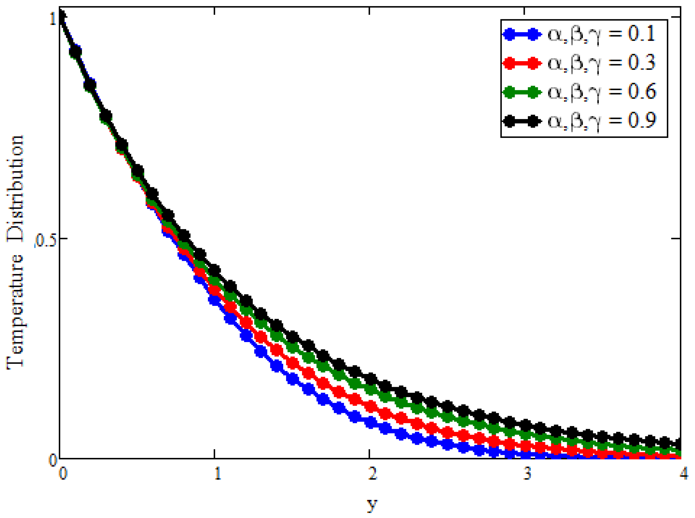
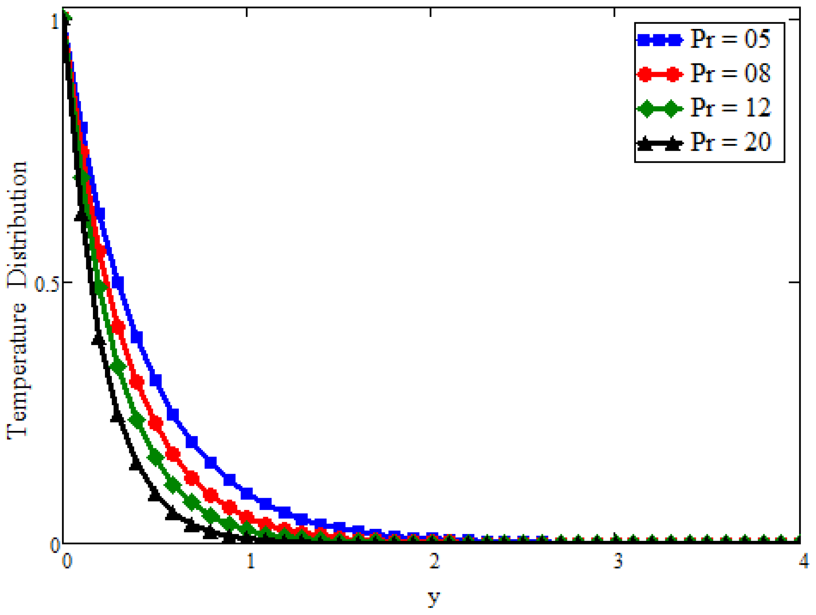
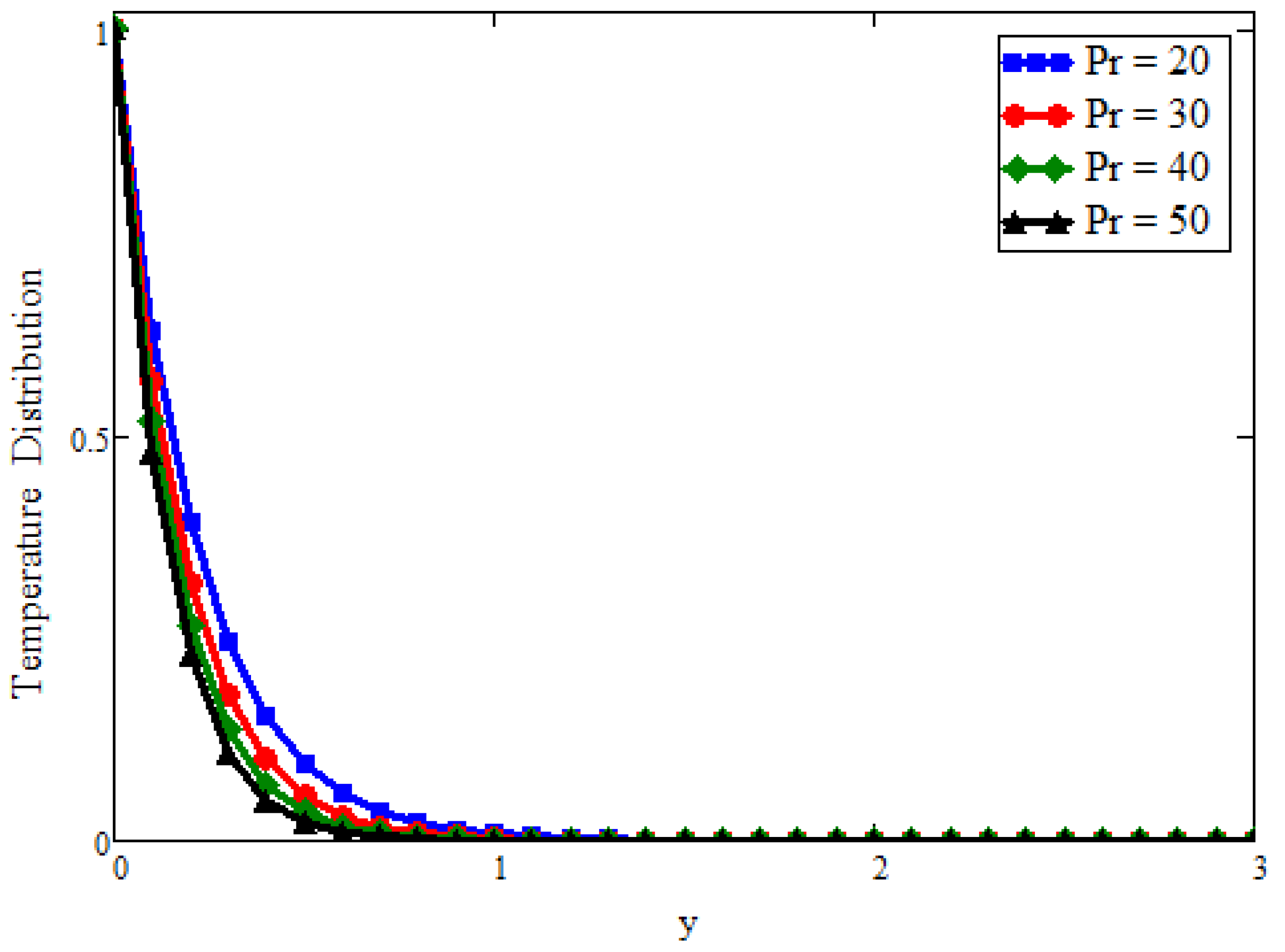
4.1. Temperature Field’s Outcome

By using the Laplace transform of Equations (18) and (19), we get

$$\begin{array}{c}\hfill \mathrm{Pr}s\overline{\tilde{\theta }}(Y,s)=-{\overline{\tilde{q}}}_Y(Y,s),\end{array}$$

(23)

and

$$\begin{array}{c}\hfill \overline{\tilde{q}}(Y,s)=-s^{\beta }{(1-a{s}^{-\alpha })}^{\gamma }{\overline{\tilde{\theta }}}_Y.\end{array}$$

(24)

By introducing Equation (24) into Equation (23), we get

$$\begin{array}{c}\hfill {\overline{\tilde{\theta }}}_{YY}(Y,s)-\frac{\overline{\tilde{\theta }}(Y,s)\mathrm{Pr}s}{s^{\beta }{(1-a{s}^{-\alpha })}^{\gamma }}=0,\end{array}$$

(25)

satisfy the following constraints:

$$\begin{array}{c}\hfill \overline{\tilde{\theta }}(\infty ,s)=0,\overline{\tilde{\theta }}(0,s)=\frac{1}{s}.\end{array}$$

(26)

With the general solution of Equation (25) subject to the constraints (26), we get

$$\begin{array}{c}\hfill \overline{\tilde{\theta }}(Y,s)=\frac{1}{s}{e}^{-Y\sqrt{\frac{Prs}{s^{\beta {(1-a{s}^{-\alpha })}^{\gamma }}}}}.\end{array}$$

(27)

We cannot find the inverse Laplace transform directly from the table of Laplace transform. Therefore, Equation (27) is expressed in series expression as follows:

$$\begin{array}{c}\hfill \overline{\tilde{\theta }}(Y,s)=\frac{1}{s}+\sum _{\ell =1}^{\infty }\sum _{p=0}^{\infty }\frac{{(-Y)}^{\ell }{\left(\mathrm{Pr}\right)}^{\frac{\ell }{2}}{\left(a\right)}^p}{\ell !p!s^{\frac{\beta \ell }{2}-\frac{\ell }{2}+\alpha p+1}}\frac{\mathsf{\Gamma }(\frac{\gamma \ell }{2}+p)}{\mathsf{\Gamma }\left(\frac{\gamma \ell }{2}\right)}.\end{array}$$

(28)

Taking the Laplace inverse transform of Equation (28), we have

$$\begin{array}{c}\hfill \tilde{\theta }(Y,t)=1+\sum _{\ell =1}^{\infty }\sum _{p=0}^{\infty }\frac{{(-Y)}^{\ell }{\left(\mathrm{Pr}\right)}^{\frac{\ell }{2}}{\left(a\right)}^p{t}^{\frac{\beta \ell }{2}-\frac{\ell }{2}+\alpha p}}{\ell !p!\mathsf{\Gamma }(\frac{\beta \ell }{2}-\frac{\ell }{2}+\alpha p+1)}\frac{\mathsf{\Gamma }(\frac{\gamma \ell }{2}+p)}{\mathsf{\Gamma }\left(\frac{\gamma \ell }{2}\right)},\end{array}$$

(29)

which satisfy the boundary condition.

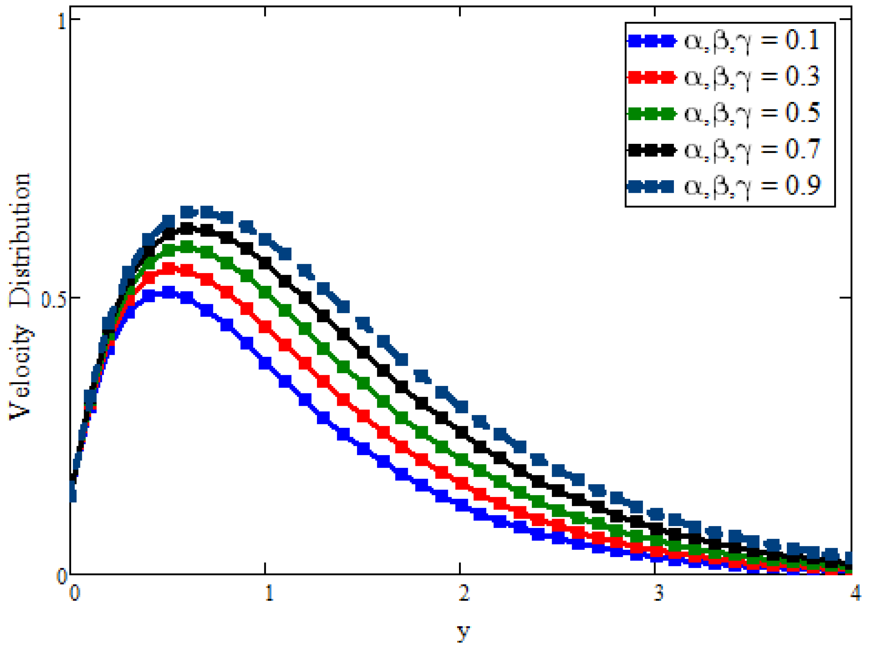
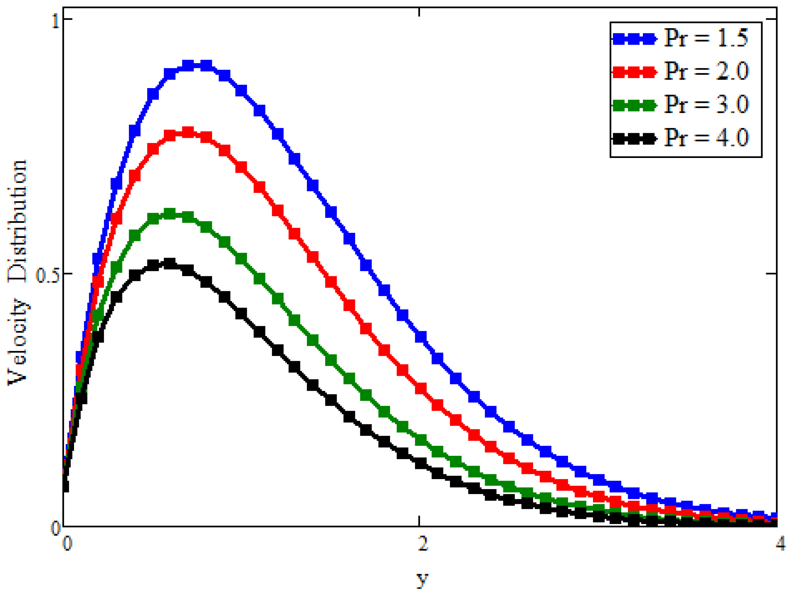
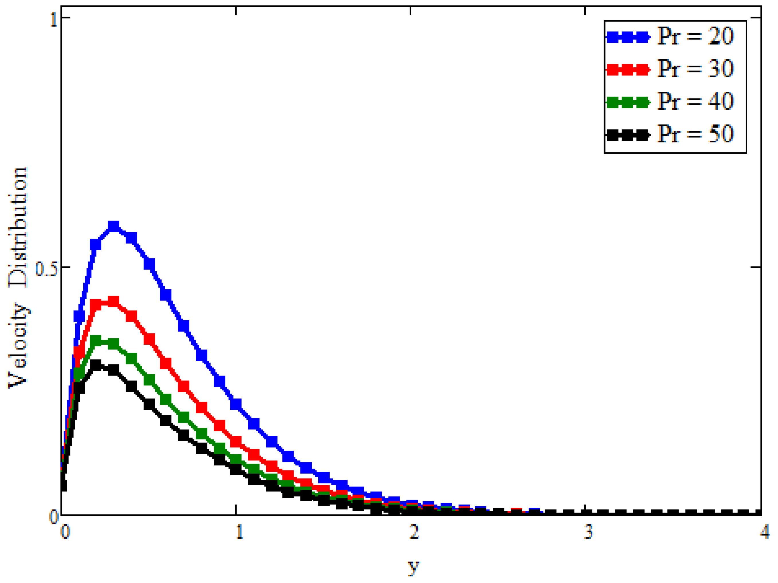
4.2. Velocity Field’s Outcome

By applying the Laplace transform of Equation (17), we have

$$\begin{array}{c}\hfill \left[D^2-\frac{s}{a_1}\right]\overline{\tilde{V}}(Y,s)=-\frac{\mathrm{Gr}}{a_1}\overline{\tilde{\theta }}(Y,s),\end{array}$$

(30)

satisfy following constraints:

$$\begin{array}{c}\hfill \overline{\tilde{V}}(\infty ,s)=0,\overline{\tilde{V}}(0,s)=\frac{\omega }{s^2+{\omega }^2}.\end{array}$$

(31)

From Equations (30) and (31), we acquire the solution of velocity:

$$\begin{array}{c}\hfill \overline{\tilde{V}}(Y,s)=\frac{\omega }{s^2+{\omega }^2}{e}^{-Y\sqrt{\frac{s}{a_1}}}-\frac{\mathrm{Gr}}{s^2}\frac{e^{-Y\sqrt{\frac{s}{a_1}}}}{(1-\frac{a_1\mathrm{Pr}}{s^{\beta {(1-a{s}^{-\alpha })}^{\gamma }}})}+\frac{\mathrm{Gr}}{s^2}\frac{e^{-Y\sqrt{\frac{\mathrm{Pr}s}{s^{\beta {(1-a{s}^{-\alpha })}^{\gamma }}}}}}{(1-\frac{a_1\mathrm{Pr}}{s^{\beta {(1-a{s}^{-\alpha })}^{\gamma }}})},\end{array}$$

(32)

where $a_1=(1+\frac{1}{{\gamma }_1}).$

Equation (32) can be expressed as,

$$\begin{array}{c}\hfill \overline{\tilde{V}}(Y,s)={\overline{\tilde{V}}}_1(Y,s)+{\overline{\tilde{V}}}_2(Y,s)+{\overline{\tilde{V}}}_3(Y,s)+{\overline{\tilde{V}}}_4(Y,s),\end{array}$$

(33)

where ${\overline{\tilde{V}}}_1,{\overline{\tilde{V}}}_2,{\overline{\tilde{V}}}_3\mathrm{and}{\overline{\tilde{V}}}_4$ are expressed in a suitable form.

$$\begin{array}{c}\hfill {\overline{\tilde{V}}}_1(Y,s)=\frac{1}{2\omega }\sum _{k=0}^{\infty }\sum _{k_1=0}^{\infty }\frac{{(-Y)}^k}{k!{\left(i\omega \right)}^{k_1}{\left(a_1\right)}^{\frac{k}{2}}{s}^{\frac{-k}{2}-k_1}},\end{array}$$

(34)

$$\begin{array}{c}\hfill {\overline{\tilde{V}}}_2(Y,s)=\frac{1}{2\omega }\sum _{k=0}^{\infty }\sum _{k_2=0}^{\infty }\frac{{(-Y)}^k}{k!{(-i\omega )}^{k_2}{\left(a_1\right)}^{\frac{k}{2}}{s}^{\frac{-k}{2}-k_2}},\end{array}$$

(35)

$$\begin{array}{c}\hfill {\overline{\tilde{V}}}_3(Y,s)=-\mathrm{Gr}\sum _{k=0}^{\infty }\sum _{{\rho }_1=0}^{\infty }\sum _{{\rho }_2=0}^{\infty }\frac{{(-Y)}^k{\left(a_1\right)}^{{\rho }_1-\frac{k}{2}}{\left(\mathrm{Pr}\right)}^{{\rho }_1}{\left(a\right)}^{{\rho }_2}}{k!{\rho }_2!s^{\beta {\rho }_1+\alpha {\rho }_2-\frac{k}{2}+2}}\frac{\mathsf{\Gamma }(\gamma {\rho }_1+{\rho }_2)}{\mathsf{\Gamma }\left(\gamma {\rho }_1\right)},\end{array}$$

(36)

$$\begin{array}{c}\hfill {\overline{\tilde{V}}}_4(Y,s)=\mathrm{Gr}\sum _{{\lambda }_1=0}^{\infty }\sum _{{\lambda }_2=0}^{\infty }\sum _{{\rho }_1=0}^{\infty }\sum _{{\rho }_2=0}^{\infty }\frac{{(-Y)}^{{\lambda }_1}{\left(a_1\right)}^{{\rho }_1}{\left(\mathrm{Pr}\right)}^{{\rho }_1+\frac{{\lambda }_1}{2}}{\left(a\right)}^{{\lambda }_2+{\rho }_2}}{{\lambda }_1!{\lambda }_2!{\rho }_2!s^{\frac{\beta {\lambda }_1}{2}-\frac{{\lambda }_1}{2}+\alpha {\lambda }_2+\beta {\rho }_1+\alpha {\rho }_2+2}}\frac{\mathsf{\Gamma }(\frac{\gamma {\lambda }_1}{2}+{\lambda }_2)}{\mathsf{\Gamma }\left(\frac{\gamma {\lambda }_1}{2}\right)}\frac{\mathsf{\Gamma }(\gamma {\rho }_1+{\rho }_2)}{\mathsf{\Gamma }\left(\gamma {\rho }_1\right)}.\end{array}$$

(37)

Next, taking the inverse of Equations (33) and (37),

$$\begin{array}{c}\hfill \tilde{V}(Y,t)={\tilde{V}}_1(Y,t)+{\tilde{V}}_2(Y,t)+{\tilde{V}}_3(Y,t)+{\tilde{V}}_4(Y,t),\end{array}$$

(38)

$$\begin{array}{c}\hfill {\tilde{V}}_1(Y,t)=\frac{1}{2\omega }\sum _{k=0}^{\infty }\sum _{k_1=0}^{\infty }\frac{{(-Y)}^k}{k!{\left(i\omega \right)}^{k_1}{\left(a_1\right)}^{\frac{k}{2}}}\frac{t^{\frac{-k}{2}-k_1-1}}{\mathsf{\Gamma }(\frac{-k}{2}-k_1)},\end{array}$$

(39)

$$\begin{array}{c}\hfill {\tilde{V}}_2(Y,t)=\frac{1}{2\omega }\sum _{k=0}^{\infty }\sum _{k_2=0}^{\infty }\frac{{(-Y)}^k}{k!{(-i\omega )}^{k_2}{\left(a_1\right)}^{\frac{k}{2}}}\frac{t^{\frac{-k}{2}-k_2-1}}{\mathsf{\Gamma }(\frac{-k}{2}-k_2)},\end{array}$$

(40)

$$\begin{array}{c}\hfill {\tilde{V}}_3(Y,t)=-\mathrm{Gr}\sum _{k=0}^{\infty }\sum _{{\rho }_1=0}^{\infty }\sum _{{\rho }_2=0}^{\infty }\frac{{(-Y)}^k{\left(a_1\right)}^{{\rho }_1-\frac{k}{2}}{\left(\mathrm{Pr}\right)}^{{\rho }_1}{\left(a\right)}^{{\rho }_2}{t}^{\beta {\rho }_1+\alpha {\rho }_2-\frac{k}{2}+1}}{k!{\rho }_2!\mathsf{\Gamma }(\beta {\rho }_1+\alpha {\rho }_2-\frac{k}{2}+2)}\frac{\mathsf{\Gamma }(\gamma {\rho }_1+{\rho }_2)}{\mathsf{\Gamma }\left(\gamma {\rho }_1\right)},\end{array}$$

(41)

$$\begin{array}{c}\hfill {\tilde{V}}_4(Y,t)=\mathrm{Gr}\sum _{{\lambda }_1=0}^{\infty }\sum _{{\lambda }_2=0}^{\infty }\sum _{{\rho }_1=0}^{\infty }\sum _{{\rho }_2=0}^{\infty }\frac{{(-Y)}^{{\lambda }_1}{\left(a_1\right)}^{{\rho }_1}{\left(\mathrm{Pr}\right)}^{{\rho }_1+\frac{{\lambda }_1}{2}}{\left(a\right)}^{{\lambda }_2+{\rho }_2}{t}^{\frac{\beta {\lambda }_1}{2}-\frac{{\lambda }_1}{2}+\alpha {\lambda }_2+\beta {\rho }_1+\alpha {\rho }_2+1}}{{\lambda }_1!{\lambda }_2!{\rho }_2!\mathsf{\Gamma }(\frac{\beta {\lambda }_1}{2}-\frac{{\lambda }_1}{2}+\alpha {\lambda }_2+\beta {\rho }_1+\alpha {\rho }_2+2)}\\ \hfill \frac{\mathsf{\Gamma }(\frac{\gamma {\lambda }_1}{2}+{\lambda }_2)}{\mathsf{\Gamma }\left(\frac{\gamma {\lambda }_1}{2}\right)}\frac{\mathsf{\Gamma }(\gamma {\rho }_1+{\rho }_2)}{\mathsf{\Gamma }\left(\gamma {\rho }_1\right)}.\end{array}$$

(42)

5. Graphically Results and Discussion

The Prabhakar fractional derivative was used to analyze the behavior of Casson fluid using the Laplace transform method. To get a physical understanding of flow parameters, particularly fractional parameters, and to look at some additional graphs from [2,3,4,5,6,7,8,9,10,11,12,13].

For accuracy and validation of temperature and velocity, Figure 2 and Figure 3 are presented. These figures portrayed the comparison between classical solutions obtained by Khalid et al. [42] and the present results when fractional parameters $\beta =\gamma =0$ and $\alpha =1$. It is found that our general results in the limiting form are validated and correct. Figure 4 and Figure 5 depict the comparison between classical solutions obtained by Khalid et al. [42] and the present results for different values of fractional parameters. The temperature of the fluid for different values of fractional parameters is obtained by considering small and large values of the time. It is evident from the figures that for a small time, the fluid properties can be increased, and for a large time, fluid properties can be decreased.Moreover, it is concluded that the fractional parameters control the boundary layer thickness and show the dual behavior for different values of the time. In Figure 6, we have another comparison that shows maximum velocity can be achieved in the mainstream region away from the plate with the larger values of fractional parameters.

Figure 7 and Figure 8 are plotted for the influence of fractional parameters on temperature and velocity, respectively. The fractional approach is responsible for exhibiting the memory of the fluid properties. It is clear from the figures that for smaller fractional parameters that maximum memory can be achieved at the present time, and for larger values of fractional parameters, the boundary layers approach the classical model. However, it is concluded that the fractional solutions show behavior for a different time. Therefore, we can say that the fractional approach has an advantage in controlling the boundary layers, and this fact can be used in the fitting of real data. As we increase the value of $\mathrm{Gr}$ in Figure 9, the velocity increases. This is because when $\mathrm{Gr}$ increases, the buoyancy forces become much greater, resulting in more convection and ultimately velocity increases.

When the value of $\mathrm{Pr}$ is increased in Figure 10, the temperature drops. Physically, increasing the value of Pr makes the fluid thicker, resulting in the lowest thickness of the thermal boundary layer. Figure 11 depicts the effect of the velocity profile on $\mathrm{Pr}$. Velocity decreases as $\mathrm{Pr}$ increases. The temperature and velocity profiles for different larger values of Prandtl number Pr are shown in Figure 12 and Figure 13 when the other parameters are fixed. It is observed that the temperature of the fluid decreases with increasing Prandtl number and velocity of fluid increases with increases of the values of Prandtl number $\mathrm{Pr}$. The thickness of the thermal boundary layer is found to be a minimum near the plate. Fluids with a high $\mathrm{Pr}$ number have a higher viscosity and low thermal conductivity limits because of thicker fluid. It is concluded that the Prabhakar fractional model of temperature and velocity field holds for smaller and larger Prandtl numbers. Figure 14 depicts the graphical results for the fractional parameter $\alpha$ and phase angle $\omega t$. The fluid appears to be oscillating between 0 and 1. These variations near the plate are extreme and rise for further values of independent variable y. We have concentrated more on such results to illustrate them on the values of $\alpha$ = 0.2, 0.4, 0.6, 0.8 and $\omega t$ = 0, $\frac{\pi }{4},\frac{\pi }{2}$ and $\pi .$

6. Conclusions

The analytical solutions of fractional partial differential equations that emerge in Casson fluid phenomena are the subject of this research. The Prabhakar fractional model of Casson fluid through generalized Fourier law for oscillating surface with Laplace transform methods. Graphical representations have been used to discuss some of the physical effects of flow characteristics:

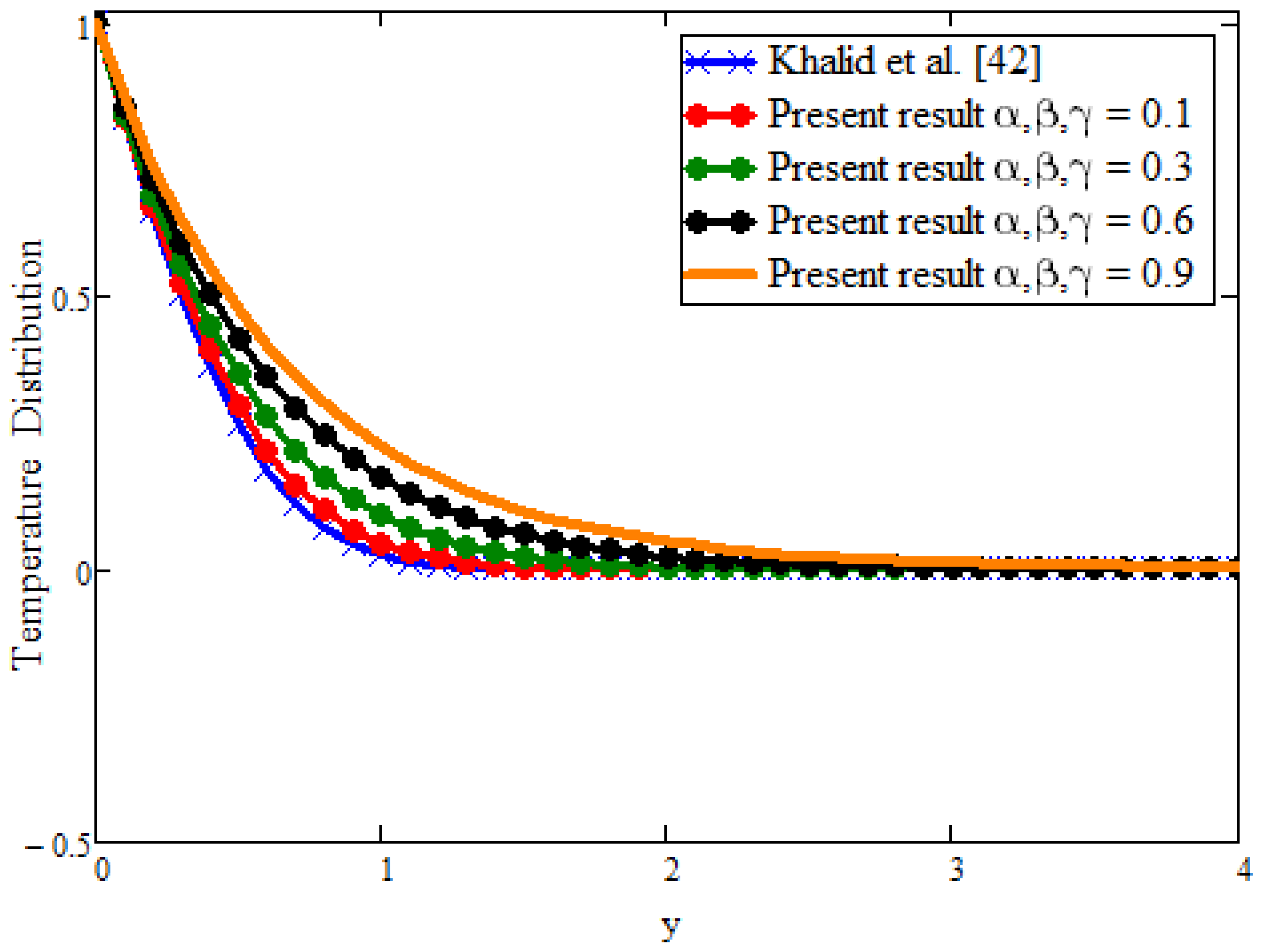
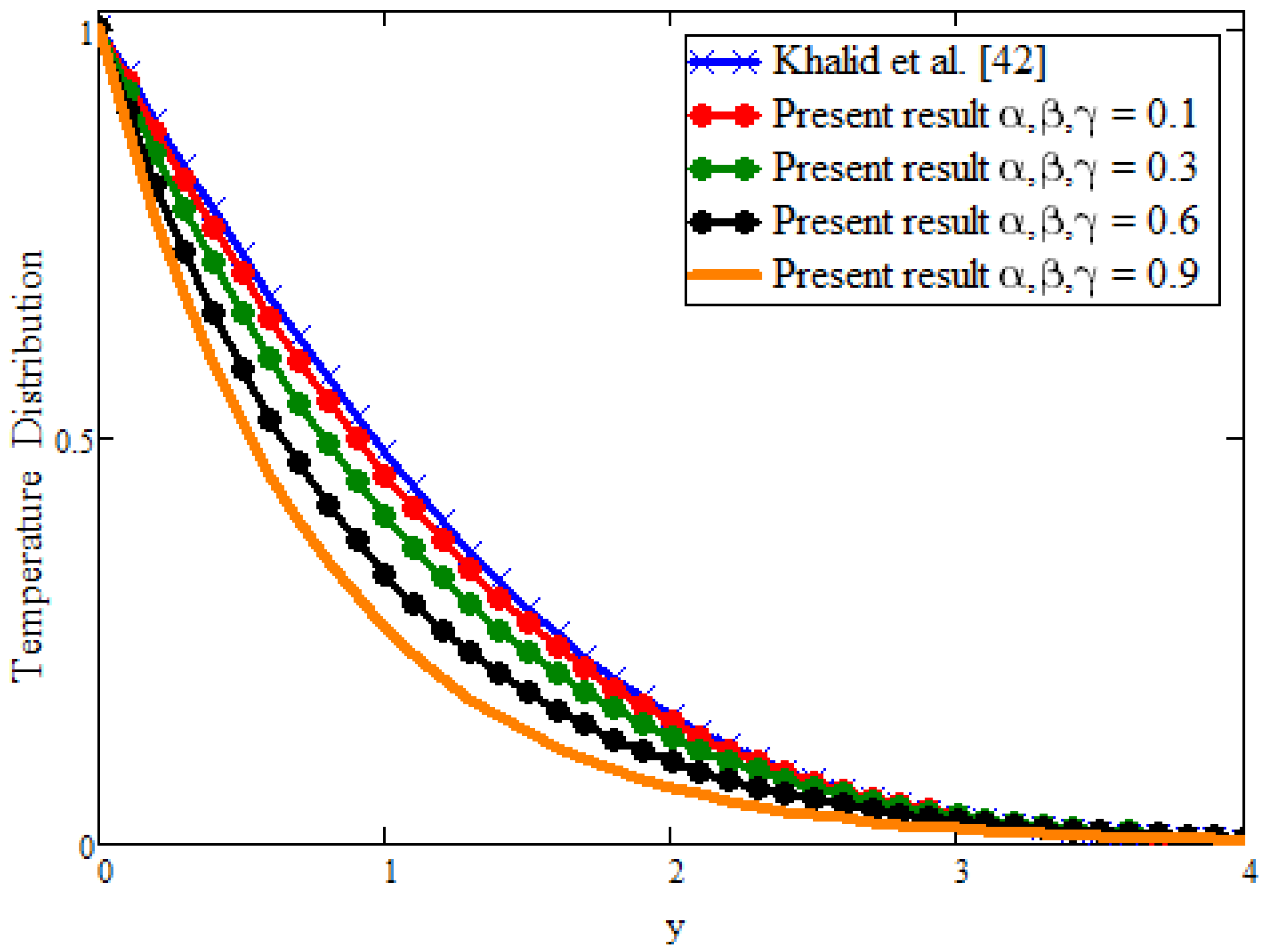
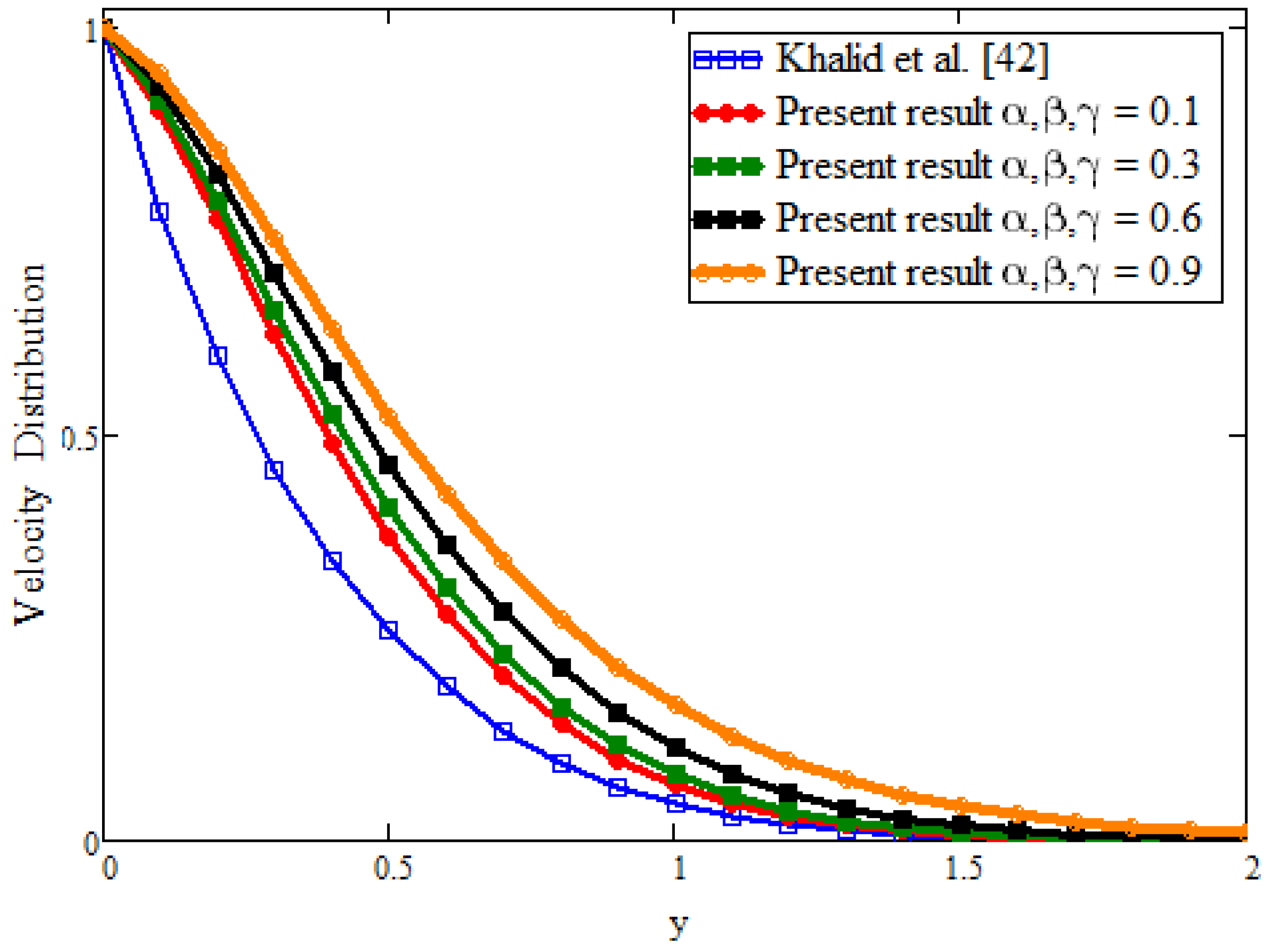
• For fractional parameters, the energy and momentum boundary layer can be controlled with different values of the time.
• The Prabhakar fractional model holds for small and larger values of the Prandtl number.
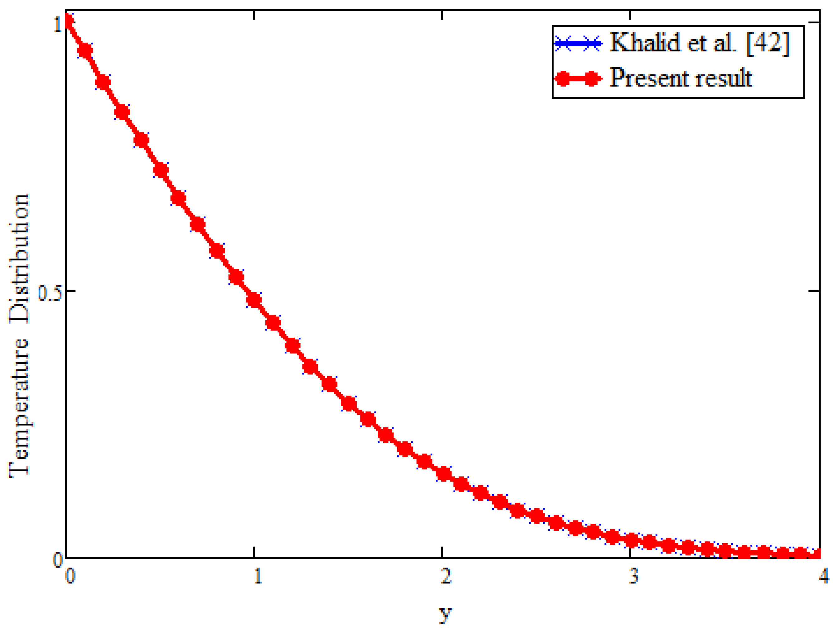
• For validation, recent results are recovered and presented graphically in the graphic section and show good agreement.
• The fractional derivative approach can be useful in fitting the real data where needed instead of classical approach.
• In the limiting case, when fractional parameters are taken $\beta =\gamma$ = 0 and $\alpha$ = 1 for both velocity and temperature, we find the solutions obtained with ordinary derivatives from the existing literature.
• This model is a linear fractional model with oscillation at the boundary displaying the laminar flow. It is possible when the fractional model is non-linear with turbulence and not handled with integral transform. Then, in order to handle the turbulence, some numerical methods are required, such as finite element method, RK-4, etc.

References

1. Casson, N. A flow equation for pigment-oil suspensions of the printing ink type. In Rheol. Disperse Syst.; Pergamon Press: Oxford, UK, 1959. [Google Scholar]
2. Pramanik, S. Casson fluid flow and heat transfer past an exponentially porous stretching surface in presence of thermal radiation. Ain Shams Eng. J. 2014, 5, 205–212. [Google Scholar] [CrossRef] [Green Version]
3. Dash, R.K.; Mehta, K.N.; Jayaraman, G. Casson fluid flow in a pipe filled with a homogeneous porous medium. Int. J. Eng. Sci. 1996, 34, 1145–1156. [Google Scholar] [CrossRef]
4. Sheikh, N.A.; Ching, D.L.C.; Khan, I.; Kumar, D.; Nisar, K.S. A new model of fractional Casson fluid based on generalized Fick’s and Fourier’s laws together with heat and mass transfer. Alex. Eng. J. 2020, 59, 2865–2876. [Google Scholar] [CrossRef]
5. Ndolane, S.E.N.E. A new approach for the solutions of the fractional generalized Casson fluid model described by Caputo fractional operator. Adv. Theory Nonlinear Anal. Its Appl. 2020, 4, 373–384. [Google Scholar]
6. Arif, M.; Kumam, P.; Kumam, W.; Khan, I.; Ramzan, M. A Fractional Model of Casson Fluid with Ramped Wall Temperature: Engineering Applications of Engine Oil. Comput. Math. Methods 2021, e1162. [Google Scholar] [CrossRef]
7. Ali, F.; Sheikh, N.A.; Khan, I.; Saqib, M. Solutions with Wright function for time fractional free convection flow of Casson fluid. Arab. J. Sci. Eng. 2017, 42, 2565–2572. [Google Scholar] [CrossRef]
8. Raza, A.; Khan, S.U.; Farid, S.; Khan, M.I.; Sun, T.C.; Abbasi, A.; Khan, M.I.; Malik, M.Y. Thermal activity of conventional Casson nanoparticles with ramped temperature due to an infinite vertical plate via fractional derivative approach. Case Stud. Therm. Eng. 2021, 27, 101191. [Google Scholar] [CrossRef]
9. Khan, I.; Shah, N.A.; Vieru, D. Unsteady flow of generalized Casson fluid with fractional derivative due to an infinite plate. Eur. Phys. J. Plus 2016, 131, 1–12. [Google Scholar] [CrossRef]
10. Saqib, M.; Shafie, S.; Khan, I.; Chu, Y.M.; Nisar, K.S. Symmetric MHD channel flow of nonlocal fractional model of BTF containing hybrid nanoparticles. Symmetry 2020, 12, 663. [Google Scholar] [CrossRef]
11. Koffi, M.; Andreopoulos, Y.; Jiji, L. Heat transfer enhancement by induced vortices in the vicinity of a rotationally oscillating heated plate. Int. J. Heat Mass Transf. 2017, 112, 862–875. [Google Scholar] [CrossRef]
12. Akcay, S.; Akdag, U.; Palancioglu, H. Experimental investigation of mixed convection on an oscillating vertical flat plate. Int. Commun. Heat Mass Transf. 2020, 113, 104528. [Google Scholar] [CrossRef]
13. Song, Y.Q.; Raza, A.; Al-Khaled, K.; Farid, S.; Khan, M.I.; Khan, S.U.; Shi, Q.H.; Malik, M.Y.; Khan, M.I. Significances of exponential heating and Darcy’s law for second grade fluid flow over oscillating plate by using Atangana-Baleanu fractional derivatives. Case Stud. Therm. Eng. 2021, 27, 101266. [Google Scholar] [CrossRef]
14. Ali, F.; Khan, I.; Shafie, S. Closed form solutions for unsteady free convection flow of a second grade fluid over an oscillating vertical plate. PLoS ONE 2014, 9, e85099. [Google Scholar] [CrossRef] [Green Version]
15. Haider, M.I.; Asjad, M.I.; Ali, R.; Ghaemi, F.; Ahmadian, A. Heat transfer analysis of micropolar hybrid nanofluid over an oscillating vertical plate and Newtonian heating. J. Therm. Anal. Calorim. 2021, 144. [Google Scholar] [CrossRef]
16. Shah, N.A.; Khan, I. Heat transfer analysis in a second grade fluid over and oscillating vertical plate using fractional Caputo–Fabrizio derivatives. Eur. Phys. J. C 2016, 76, 1–11. [Google Scholar] [CrossRef] [Green Version]
17. Sheikholeslami, M.; Kataria, H.R.; Mittal, A.S. Effect of thermal diffusion and heat-generation on MHD nanofluid flow past an oscillating vertical plate through porous medium. J. Mol. Liq. 2018, 257, 12–25. [Google Scholar] [CrossRef]
18. Fang, Z.W.; Sun, H.W.; Wang, H. A fast method for variable-order Caputo fractional derivative with applications to time-fractional diffusion equations. Comput. Math. Appl. 2020, 80, 1443–1458. [Google Scholar] [CrossRef]
19. Dassios, I.; Baleanu, D. Optimal solutions for singular linear systems of Caputo fractional differential equations. Math. Methods Appl. Sci. 2021, 44, 884–7896. [Google Scholar] [CrossRef] [Green Version]
20. Ali, R.; Akgül, A.; Asjad, M.I. Power law memory of natural convection flow of hybrid nanofluids with constant proportional Caputo fractional derivative due to pressure gradient. Pramana 2020, 94, 1–11. [Google Scholar] [CrossRef]
21. Baleanu, D.; Jajarmi, A.; Mohammadi, H.; Rezapour, S. A new study on the mathematical modelling of human liver with Caputo–Fabrizio fractional derivative. Chaos Solitons Fractals 2020, 134, 109705. [Google Scholar] [CrossRef]
22. Alizadeh, S.; Baleanu, D.; Rezapour, S. Analyzing transient response of the parallel RCL circuit by using the Caputo–Fabrizio fractional derivative. Adv. Differ. Equ. 2020, 2020, 55. [Google Scholar] [CrossRef]
23. Shah, K.; Jarad, F.; Abdeljawad, T. On a nonlinear fractional order model of dengue fever disease under Caputo-Fabrizio derivative. Alex. Eng. J. 2020, 59, 2305–2313. [Google Scholar] [CrossRef]
24. Abdeljawad, T.; Hajji, M.A.; Al-Mdallal, Q.M.; Jarad, F. Analysis of some generalized ABC–fractional logistic models. Alex. Eng. J. 2020, 59, 2141–2148. [Google Scholar] [CrossRef]
25. Thabet, S.T.; Abdo, M.S.; Shah, K.; Abdeljawad, T. Study of transmission dynamics of COVID-19 mathematical model under ABC fractional order derivative. Results Phys. 2020, 19, 103507. [Google Scholar] [CrossRef] [PubMed]
26. Ghanbari, B.; Atangana, A. A new application of fractional Atangana–Baleanu derivatives: Designing ABC-fractional masks in image processing. Phys. A Stat. Mech. Appl. 2020, 542, 123516. [Google Scholar] [CrossRef]
27. Garra, R.; Gorenflo, R.; Polito, F.; Tomovski, Ž. Hilfer–Prabhakar derivatives and some applications. Appl. Math. Comput. 2014, 242, 576–589. [Google Scholar] [CrossRef] [Green Version]
28. Benchohra, M.; Bouriah, S.; Nieto, J.J. Terminal value problem for differential equations with Hilfer–Katugampola fractional derivative. Symmetry 2019, 11, 672. [Google Scholar] [CrossRef] [Green Version]
29. Asif, M.; Ul Haq, S.; Islam, S.; Abdullah Alkanhal, T.; Khan, Z.A.; Khan, I.; Nisar, K.S. Unsteady flow of fractional fluid between two parallel walls with arbitrary wall shear stress using Caputo–Fabrizio derivative. Symmetry 2019, 11, 449. [Google Scholar] [CrossRef] [Green Version]
30. Polito, F.; Tomovski, Z. Some properties of Prabhakar-type fractional calculus operators. arXiv 2015, arXiv:1508.03224. [Google Scholar] [CrossRef]
31. Elnaqeeb, T.; Shah, N.A.; Mirza, I.A. Natural convection flows of carbon nanotubes nanofluids with Prabhakar-like thermal transport. Math. Methods Appl. Sci. 2020. [Google Scholar] [CrossRef]
32. Shah, N.A.; Fetecau, C.; Vieru, D. Natural convection flows of Prabhakar-like fractional Maxwell fluids with generalized thermal transport. J. Therm. Anal. Calorim. 2021, 143, 2245–2258. [Google Scholar] [CrossRef]
33. Eshaghi, S.; Ghaziani, R.K.; Ansari, A. Stability and dynamics of neutral and integro-differential regularized Prabhakar fractional differential systems. Comput. Appl. Math. 2020, 39, 1–21. [Google Scholar] [CrossRef]
34. Tanveer, M.; Ullah, S.; Shah, N.A. Thermal analysis of free convection flows of viscous carbon nanotubes nanofluids with generalized thermal transport: A Prabhakar fractional model. J. Therm. Anal. Calorim. 2021, 144, 2327–2336. [Google Scholar] [CrossRef]
35. Alidousti, J. Stability region of fractional differential systems with Prabhakar derivative. J. Appl. Math. Comput. 2020, 62, 135–155. [Google Scholar] [CrossRef]
36. Derakhshan, M. New Numerical Algorithm to Solve Variable-Order Fractional Integrodifferential Equations in the Sense of Hilfer-Prabhakar Derivative. Abstr. Appl. Anal. 2021, 2021, 8817794. [Google Scholar]
37. Asjad, M.I.; Sarwar, N.; Hafeez, M.B.; Sumelka, W.; Muhammad, T. Advancement of Non–Newtonian Fluid with Hybrid Nanoparticles in a Convective Channel and Prabhakar’s Fractional Derivative—Analytical Solution. Fractal Fract. 2021, 5, 99. [Google Scholar] [CrossRef]
38. Basit, A.; Asjad, M.I.; Akgül, A. Convective flow of a fractional second grade fluid containing different nanoparticles with Prabhakar fractional derivative subject to non-uniform velocity at the boundary. Math. Methods Appl. Sci. 2021. [Google Scholar] [CrossRef]
39. Wang, F.; Asjad, M.I.; Zahid, M.; Iqbal, A.; Ahmad, H.; Alsulami, M.D. Unsteady thermal transport flow of Casson nanofluids with generalized Mittag–Leffler kernel of Prabhakar’s type. J. Mater. Res. Technol. 2021, 14, 1292–1300. [Google Scholar] [CrossRef]
40. Sene, N.; Srivastava, G. Generalized Mittag–Leffler input stability of the fractional differential equations. Symmetry 2019, 11, 608. [Google Scholar] [CrossRef] [Green Version]
41. Iyiola, O.; Oduro, B.; Zabilowicz, T.; Iyiola, B.; Kenes, D. System of time fractional models for COVID-19: Modeling, analysis and solutions. Symmetry 2021, 13, 787. [Google Scholar] [CrossRef]
42. Khalid, A.; Khan, I.; Shafie, S. Exact solutions for unsteady free convection flow of Casson fluid over an oscillating vertical plate with constant wall temperature. In Abstract and Applied Analysis; Hindawi: London, UK, 2015; Volume 2015. [Google Scholar]
43. Asjad, M.I.; Basit, A.; Iqbal, A.; Shah, N.A. Advances in transport phenomena with nanoparticles and generalized thermal process for vertical plate. Phys. Scr. 2021, 96, 114001. [Google Scholar] [CrossRef]
44. Garra, R.; Garrappa, R. The Prabhakar or three parameter Mittag–Leffler function: Theory and application. Commun. Nonlinear Sci. Numer. Simul. 2018, 56, 314–329. [Google Scholar] [CrossRef] [Green Version]
Figure 1. Physical model.
Symmetry 13 02039 g001
Figure 2. Comparison of the present results with Khalid et al. [42] on temperature field. When β = γ = 0 and t = 2, α = 1 , Pr = 20, a = 0.01.
Symmetry 13 02039 g002
Figure 3. The current outcomes are compared with Khalid et al. [42] on velocity field. When β = γ = 0 and t = 0.2, Pr = 15, α = 1 , a = 0.01, ω = π 4 ,   γ 1 = 45 ,   Gr = 0.2 .
Symmetry 13 02039 g003
Figure 4. Comparison of the present results with Khalid et al. [42] on temperature field. When t = 0.2 and a = 0.01, Pr = 20.
Symmetry 13 02039 g004
Figure 5. Comparison of the present results with Khalid et al. [42] on temperature field. When t = 2 and a = 0.01, Pr = 20.
Symmetry 13 02039 g005
Figure 6. The current outcomes are compared with Khalid et al. [42] on velocity field. When t = 0.2 and a = 0.8, Pr = 20, ω = π 4 ,   γ 1 = 45 ,   Gr = 60 .
Symmetry 13 02039 g006
Figure 7. The influence of fractional parameters ( α , β , γ ) on temperature field. When t = 0.4, a = 0.002, Pr = 20.
Symmetry 13 02039 g007
Figure 8. The influence of fractional parameters ( α , β , γ ) on velocity field. When t = 0.7, Pr = 20, ω = π 4 , γ 1 = 0.8 , a = 0.1, Gr = 15.
Symmetry 13 02039 g008
Figure 9. The impacts of Grashof number Gr on velocity field. When t = 0.3, a = 0.002, Pr = 20, α = 0.5 ,   β = 0.5 ,   γ = 0.5 , ω = π 4 .
Symmetry 13 02039 g009
Figure 10. The influence of smaller Prandtl number Pr on temperature field. When t = 1, a = 0.3, α = 0.7 ,   β = 0.7 ,   γ = 0.7 .
Symmetry 13 02039 g010
Figure 11. The influence of smaller Prandtl number Pr on velocity field. When t = 0.3, α = 0.5 ,   β = 0.5 ,   γ = 0.5 , ω = π 4 , a = 0.1, γ 1 = 0.8 , Gr = 15.
Symmetry 13 02039 g011
Figure 12. The influence of larger Prandtl number Pr on temperature field. When t = 1, a = 0.3, α = 0.7 ,   β = 0.7 ,   γ = 0.7 .
Symmetry 13 02039 g012
Figure 13. The influence of larger Prandtl number Pr on velocity field. When t = 0.7, α = 0.5 ,   β = 0.5 ,   γ = 0.5 , ω = π 4 , a = 0.1 γ 1 = 3.8 ,   Gr = 15.
Symmetry 13 02039 g013
Figure 14. The influence of α and ω t on velocity field when t = 0.4, β = 0.5 ,   γ = 0.5 , a = 0.1, γ 1 = 0.5 , Pr = 12, Gr = 2.5.
Symmetry 13 02039 g014
Publisher’s Note: MDPI stays neutral with regard to jurisdictional claims in published maps and institutional affiliations.