Abstract
This study proposes a data-driven adaptive filtering method for the fault diagnosis (DDAF-FD) of discrete-time nonlinear systems and provides a simultaneous online estimation of actuator and sensor faults. First, dynamic linearization was adopted to transform the nonlinear system into a quasi-linear model, which facilitated accurate modeling of the nonlinear system. Second, a data-driven adaptive fault diagnosis method was designed under the framework of data-driven filtering and the recursive least-squares algorithm using system I/O data only, and accurate real-time estimation of two fault factors was achieved. In addition, the simulation results demonstrate the effectiveness of the proposed method. The stability was verified via the Lyapunov method.
1. Introduction
Continuous industrial development has contributed toa gradual increase in the complexity and cost of systems as well as growing demands in terms of the safety and reliability of industrial operations. Various potential abnormalities and faults must be discovered and identified in time to minimize the potential dangers of system performance degradation. Any fault in industrial systems, such as aerospace systems [1], power electronics [2], or nuclear power plants [3], can result in catastrophic damage to life and property. Therefore, fault diagnosis has high research value and is also of practical significance. Model-based fault diagnosis was proposed by Beard in 1971 [4]. Mehra and Peschon proposed a general method for fault detection and diagnosis of linear dynamic systems using residuals similar to the observer structure generated by the Kalman filter [5]. In recent decades, researchers have devoted considerable effort to fault diagnosis and achieved various results, including a detailed overview of the development of fault diagnosis and fault-tolerant control in recent years [6,7,8].
Faults are usually categorized into actuator faults, sensor faults, and object faults. Fault diagnosis includes three tasks: fault detection, fault isolation, and fault identification. Various types of fault diagnosis methods have been proposed, such as model-based methods [9], signal-based methods [10], and data-driven methods [11]. In one study, researchers proposed data-driven filtering for discrete linear time-invariant systems [12]; they used only the measured I/O data and Markov parameters, and employed a low-pass filter to produce an asymptotically unbiased estimation of the system state for the performance of fault diagnosis. A novel discrete-time estimator that can realize simultaneous estimations of the system’s state and actuator/sensor faults for linear systems of vehicle lateral dynamics was proposed in [13]. A fault detection and estimation method for robot actuators and sensors was proposed in [14]. It comprised a model-based fault detection and isolation scheme suitable for robot actuators and sensors; without adding redundant joint sensors, multiple faults in the robot actuator and sensor were detected, estimated, and isolated. An adaptive system fault/state estimation algorithm for linear time-varying systems was proposed in [15] by combining the Kalman filtering algorithm with the recursive least-squares algorithm. The effects of different forgetting factors on state estimation have been discussed in previous studies. The aforementioned studies focused on the fault diagnosis of linear systems with known models.
Model-based fault diagnosis methods require accurate system models. However, the growing complexity of actual engineering systems, as well as problems such as parameter uncertainties and unknown disturbances, reduce the likelihood of obtaining accurate mathematical descriptions of actual systems, which adversely affects fault diagnosis. Data-driven methods do not require accurate models of objects and use only I/O data to detect system faults. Therefore, data-driven fault diagnosis methods offer unique advantages for dealing with complex nonlinear systems. Kalman filtering technology has been widely used in fault diagnosis. Researchers have proposed many algorithms for the fault diagnosis of nonlinear systems, such as extend Kalman filtering (EKF) and unscented Kalman filtering (UKF) [16,17,18,19].
In [16], an actuator fault diagnosis method was proposed for nonlinear systems, which is based on the use of extended Kalman filter (EKF) to update the actuator fault estimation iteratively. However, this approach is dependent on known nonlinear dynamic models. A method based on EKF and a multi-model adaptive estimation was proposed in [17] for continuous nonlinear systems of small UAVs to realize fault detection and diagnosis of the actuators. Combined EKF with neural fuzzy networks, an adaptive estimation method is given based on EKF and multiple models [18]. A fault detection and separation method for a three-phase permanent magnet synchronous motor on the basis of a generalized UKF was proposed in [19]. This method can manage the non-linear characteristics of the system effectively, and it also offers good real-time performance, stable operation and high fault diagnosis accuracy.
The approximation of nonlinearity will inevitably result in information loss. Dynamic linearization (DL) [20,21] technology can be used to linearize discrete time nonlinear systems, and the data model can be established by using only the I/O data through the pseudo-partial-derivative identification method. In [22], local compact dynamic linearization (LOCAL-CFDL) was proposed to transform the original nonlinear non-affine system into an affine structure composed of unknown residual nonlinear time-varying terms and affine of linear parameter terms on the control input.
In this paper, a data-driven dynamic linearization (DL) approach is used to achieve the equivalent linearization of nonlinear systems and effectively retain the dynamic characteristics of the original nonlinear system. To meet the requirements of engineering practice, this study focuses on the effective use of the I/O data measured by the system to obtain fault diagnosis in nonlinear systems. Compared with the EKF method in [16], which needs the model parameters of nonlinear systems and only diagnoses actuator faults, the method based on DL only uses system I/O data and does not need a system model.
Considering the fault diagnosis problem of discrete nonlinear systems subject to simultaneous actuator and sensor faults, we propose a data-driven adaptive filtering fault diagnosis (DDAF-FD) method. By combining data-driven filtering technology with the recursive least squares algorithm, the joint estimation of states, system parameters, and fault factors is obtained. The contributions of this paper are summarized as follows:
(1) By using the dynamic linearization (DL) technique, nonlinear systems were converted into equivalent quasi-linear models, and the difficulty of modeling nonlinear systems was solved. Next, a data-driven system parameter identification method was studied via the approximation data model by using only the I/O measurement data instead of including any information on the dynamics or structure of the controlled system.
(2) The DDAF-FD scheme proposed in this paper solves the problem of actuator and sensor simultaneous fault and achieves the real-time online estimation of actuator and sensor fault factors in the system. Within the context of simultaneous faults occurring in actuators and sensors, the stability and convergence of the estimation error dynamics and the fault factors of the DDAF-FD scheme are presented rigorously through the Lyapunov method.
The rest of this paper is organized as follows: Section 2 introduces the dynamic linearization technology based on I/O data and establishes an equivalent linear model for nonlinear systems. Section 3 presents the data-driven adaptive filtering algorithm, which achieves the joint estimation of actuator and sensor fault factors. Section 4 discusses the stability analysis using the Lyapunov method. Section 5 verifies the effectiveness of the proposed approach via numerical simulation. Section 6 summarizes this paper.
2. Problem Definition
2.1. Dynamic Linearization
A discrete-time single-input single-output (SISO) nonlinear system with measurement noise can be expressed as follows:
where represents each discrete time, and denote the input and output of the system at time , respectively, are two unknown positive integers, is an unknown nonlinear function, and represents white Gaussian noise.
Next, two hypotheses are presented for the system (1).
Assumption 1.
The system (1) is taken for a smooth nonlinear function. For all the control inputs and control outputs, the partial derivatives are continuous, and the control input length L is a positive constant.
Assumption 2.
The system (1) is the Lipchitz system in a broad sense. and ,
where and is a positive constant. Further, are the length constants for controlling the output linearization and input linearization, respectively. is defined as and .
Lemma 1.
[23] If system (1) satisfies Assumptions 1 and 2, we define . When , there must be a time-varying parameter vector that transforms system (1) into the following full-format dynamic linearization model:
The nonlinear function relation of input and output is contained in the time-varying parameter vector. For each moment,has an upper bound c. Further,represents white Gaussian noise with zero mean.
2.2. Modeling
Lemma 2.
[24] The dynamic linearization model provided by (3) can be transformed into a linear time-varying system of order :
where
The selection ofand is based on the complexity of the system, the values of the two parameters become larger while more complexity of the system.
Lemma 3.
[25] The state vector is selected as follows:
that is:
Thus, the linear time-varying system provided by system (1) can be transformed into the following state space expression:
where
Therefore, a general SISO discrete nonlinear system with measurement noise can be transformed into an equivalent quasi-linear time-varying system (8).
3. Data-Driven Adaptive Filtering
3.1. System Identification
To adaptively identify the system matrix and input matrix of the quasi-linear time-varying system given by system (8), this study introduces the DDF-PI algorithm for parameter identification.
The following equation can be obtained from Equation (4):
represents the unknown parameter vector that satisfies
represents the known I/O data vector that satisfies
For the given unknown time-invariant vector (13) and measurement vector (14), the following DDF-PI algorithm can be used for parameter identification.
Through the DDF-PI algorithm provided by Equations (15)–(17),
and
can be easily obtained from the unknown parameter estimation vector. Thus, the parameters in system (8) can be identified using the DDF-PI algorithm.
3.2. State-Parameter Joint Estimation
System (8) can be rewritten as
When simultaneous actuator and sensor faults occur, the system input deviates from the expected value, and the measured value also deviates from the expected value. represents the actuator fault, and represents the sensor fault, where , , represents the actuator fault factor, and represents the sensor fault factor. When the actuator and sensor include faults (such as gain loss), the fault factors vary from 0 to 1. Here, is the output value of the system with measurement noise, where , . Let , , .
Equation (18) can be rewritten as
The proposed DDAF-FD algorithm is divided into three parts according to the recursive sequence stated below:
The recursion provided by Equations (20)–(23) is a part of Kalman filtering, which calculates the covariance matrix and state estimation gain matrix , and prepares for the next part to calculate the auxiliary variables , , , and as well as the parameter estimation gain matrix .
Inspired by the recursive least-squares estimation with the exponential forgetting factor, the recursion provided by Equations (24)–(28) calculates the parameter estimation gain matrix and auxiliary variables to prepare for the next fault parameter estimation and state estimation, where .
The recursive update given by Equations (29)–(31) is an adaptive Kalman filter, where are updated at each time k, the residual is calculated, the fault parameter estimation is updated according to Equation (30), and the state estimation is updated according to Equation (31).
4. Stability Analysis
In this section, the Lyapunov method [26] is used to prove the convergence of the proposed DDAF-FD algorithm, i.e., when , the estimation error of the state and the fault factor tend to zero. The following hypotheses are presented:
Assumption 3.
For, the matricesand the input matrixhave upper bounds,is a symmetric positive semi-definite matrix, and is a symmetric positive definite matrix with a positive lower bound.
Assumption 4.
is completely observable, andis completely controllable. When satisfies
converges exponentially.
Assumption 5.
The faultis a slowly changing fault, i.e.,.
Assumption 6.
Assuming that under the excitation of, there are constantsand, for, the matrix satisfies
where .
The above assumptions are a previous study [15]. Assuming that there is a matrix that satisfies Equations (26)–(28), under the condition of Assumption 6, for the initial condition the matrix is strictly positive definite.
Theorem 1.
Based on the above assumptions, for the dynamically linearized system (19), the adaptive filtering method (20)–(31) can be applied to achieve the effective estimation of state and fault factors, and the state and fault estimation errors converge to zero.
Proof of Theorem 1.
The state and fault parameter estimation errors are defined as
The following equation is introduced:
Equations (19), (34) and (35) are substituted into Equation (29) to obtain the following equation:
From Equations (19), (31), (34), (35) and (37), we can obtain
The following equation is obtained from Equations (30), (35) and (37):
By substituting Equation (38) into Equation (36), we can obtain
In Equation (40), the term is zero and Equation (40) can be written as
Since are uncorrelated zero-mean white Gaussian noise terms, the mathematical expectation of Equation (41) can be obtained as follows:
where is the mathematical expectation.
According to Assumption 4, for any initial value , .
By substituting Equation (36) into Equation (39), we can obtain
where
Set it has
The candidate Lyapunov function is expressed as
where
Since , are both positive definite matrices, the following equation can be obtained:
It can be seen that tends to 0 exponentially.
As is strictly positive definite, tends to 0 exponentially.
From Equation (36), we can obtain
Therefore, it can be proven that , tend to 0 exponentially, and the proposed DDAF-FD algorithm is convergent. Thus, the proof is complete. □
5. Numerical Simulations
Consider a discrete nonlinear system in which the state equation of the system contains the cubic term of the state.
where .
The simulation setting ranges from k = 0 to k = 100. The actuator fault factor parameter changes from 0 to 0.4 at k = 10. The sensor fault factor parameter changes from 0 to 0.35 at k = 10. For the simulation of this model, second-order dynamic linearization is selected. Hence, .
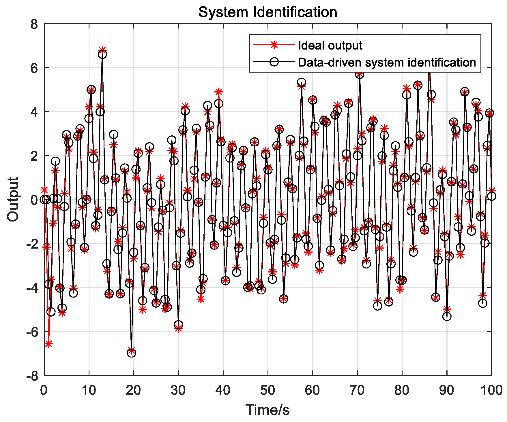
Figure 1 reflects the effectiveness of the DDF-PI algorithm. The system identification output has a very small deviation from the ideal output. Hence, the proposed system identification algorithm (DDF-PI) is sufficiently accurate.
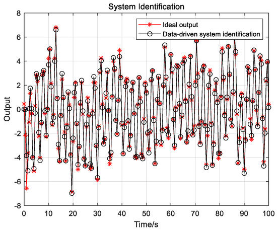
Figure 1.
Identification effects of DDF-PI algorithm.
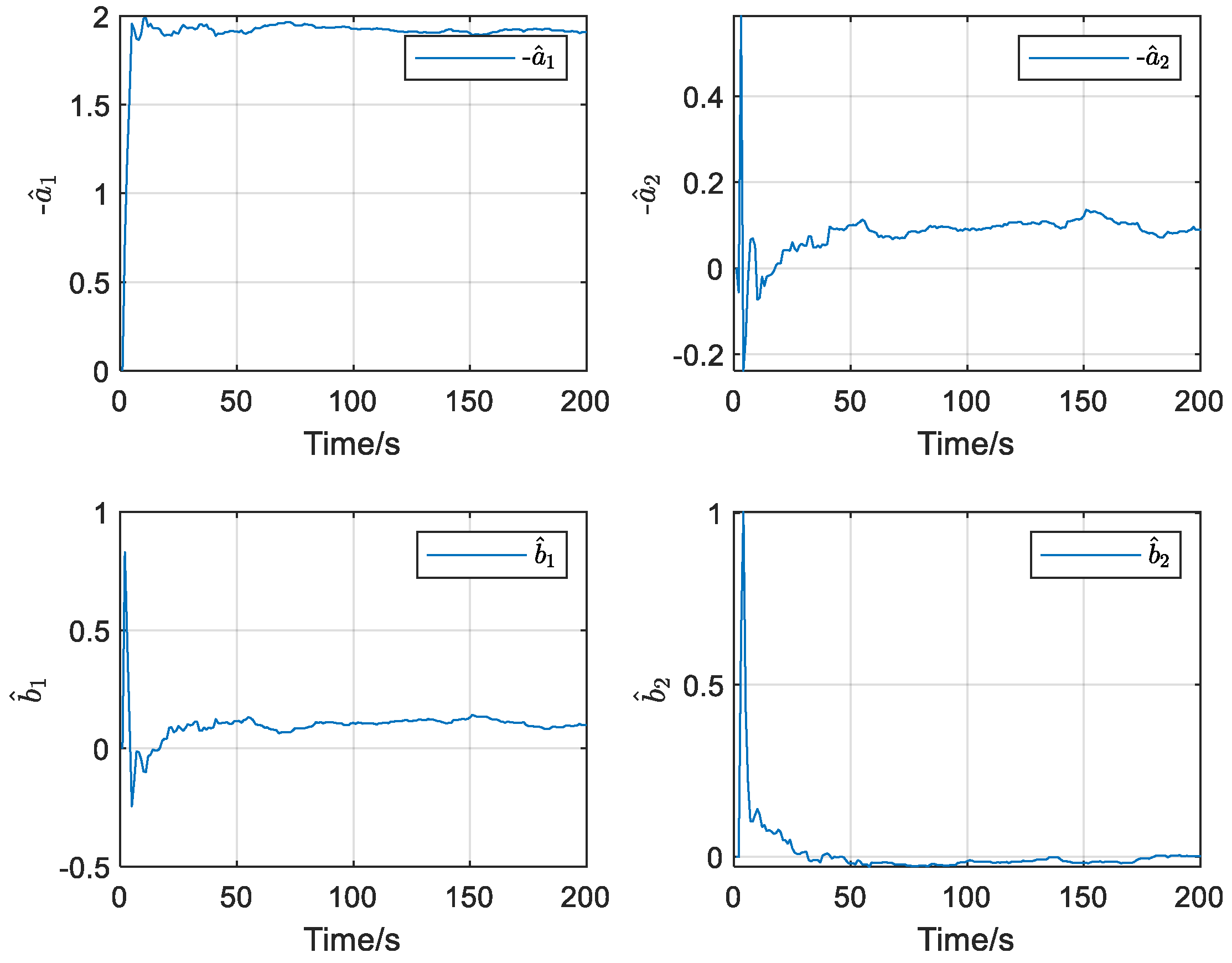
Figure 2 shows the process of identifying the parameters of the DDF-PI algorithm. As can be observed, the four system parameters eventually stabilized.
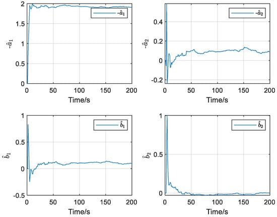
Figure 2.
Identification effects of system parameters.
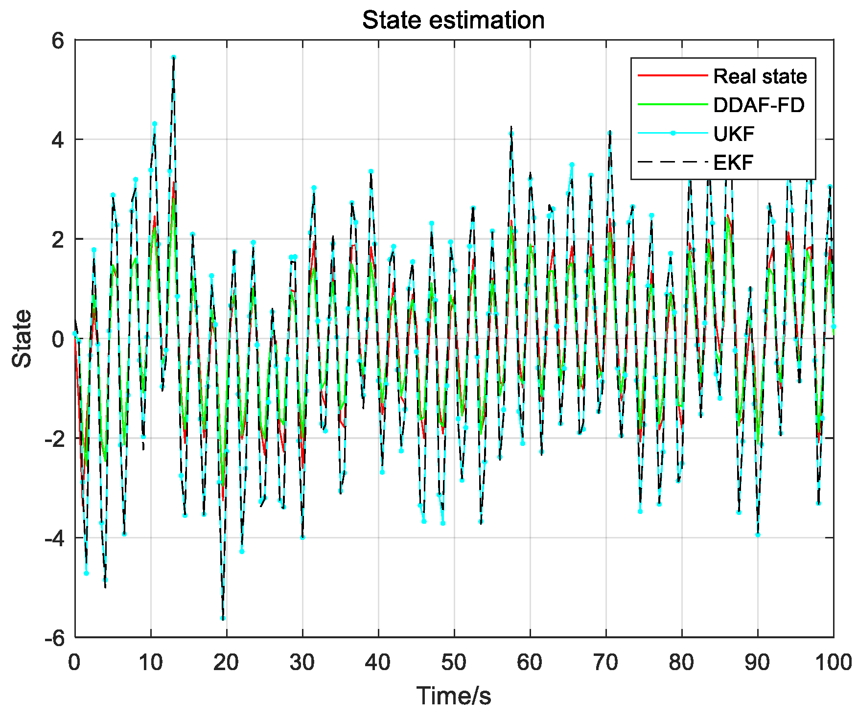
Figure 3 and Figure 4 compare the DDAF-FD algorithm with the UKF and EKF algorithms in terms of the state estimation effects. In order to quantitatively analyze the estimation effects of the three algorithms, Mean Absolute Error (MAE) was defined as
where, and respectively represent the actual state and estimated state of the system. The mean absolute error pairs of DDAF-FD, UKF and EKF methods are shown in Table 1.
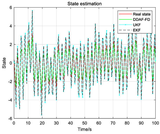
Figure 3.
Comparison of state estimation effects.
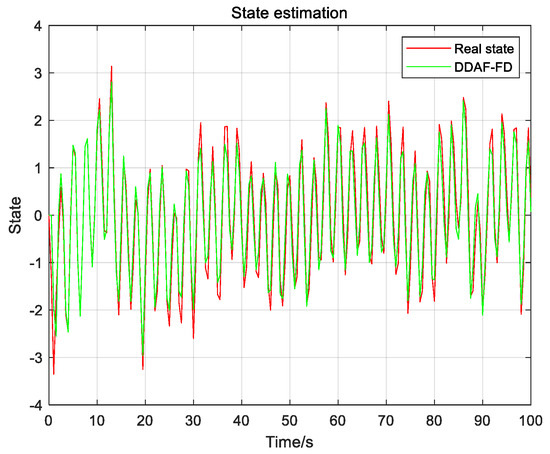
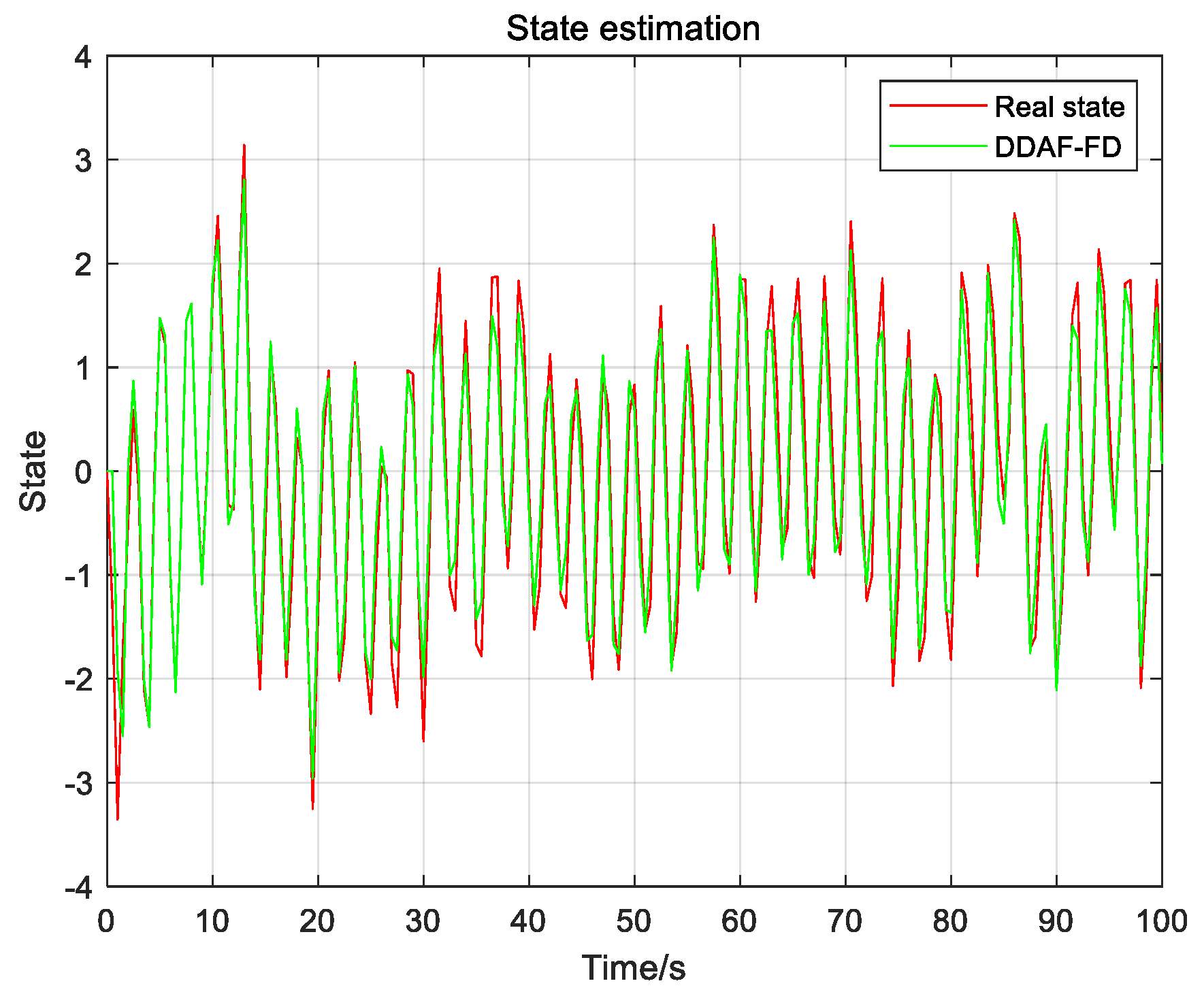
Figure 4.
State estimation effects of the DDAF-FD algorithm.

Table 1.
Mean Absolute Error.
According to the average absolute error in Table 1, the proposed DDAF-FD algorithm is superior to the UKF and EKF algorithms in terms of state estimation for a system with faults. The DDAF-FD algorithm can also perform fault estimation.
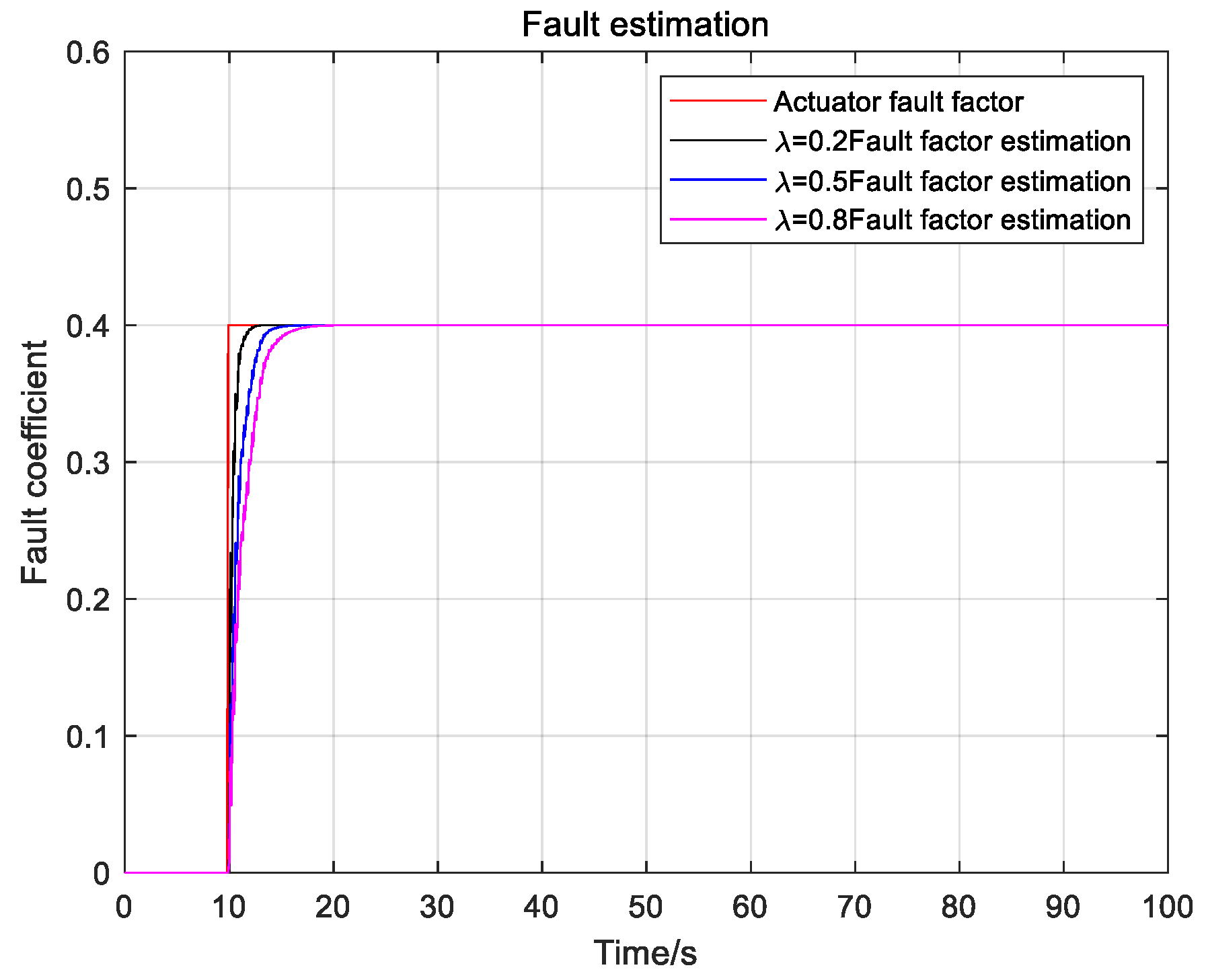
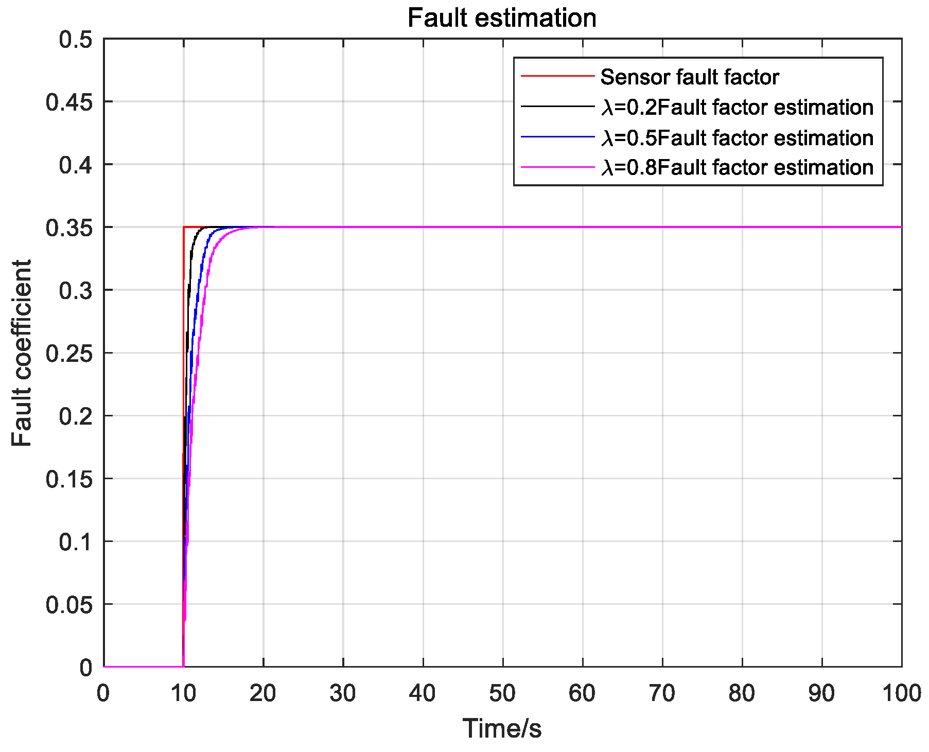
Figure 5 and Figure 6 show that the parameter estimation performance of the DDAF-FD algorithm depends on the forgetting factor . The DDAF-FD algorithm can estimate steady faults, and it can be clearly observed that when the system fails, the proposed DDAF-FD algorithm can effectively track the fault factor. As the forgetting factor decreases, the estimated convergence speed increases. Thus, the smaller the forgetting factor, the greater the sensitivity of the algorithm to system faults.
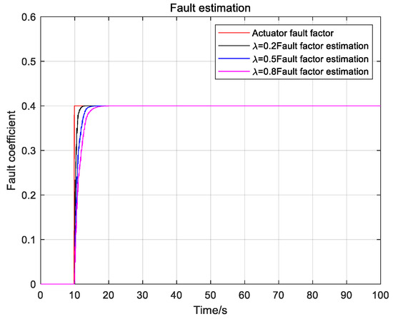
Figure 5.
Parameter estimation effects of the actuator fault factor.
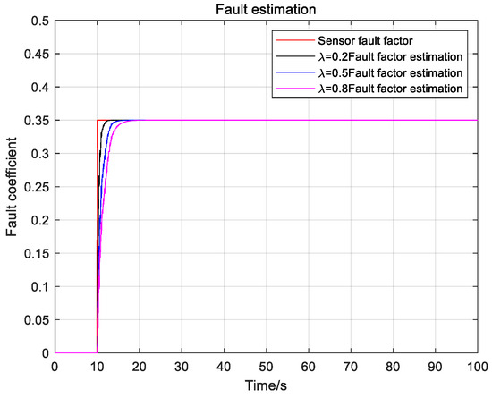
Figure 6.
Parameter estimation effects of the sensor fault factor.
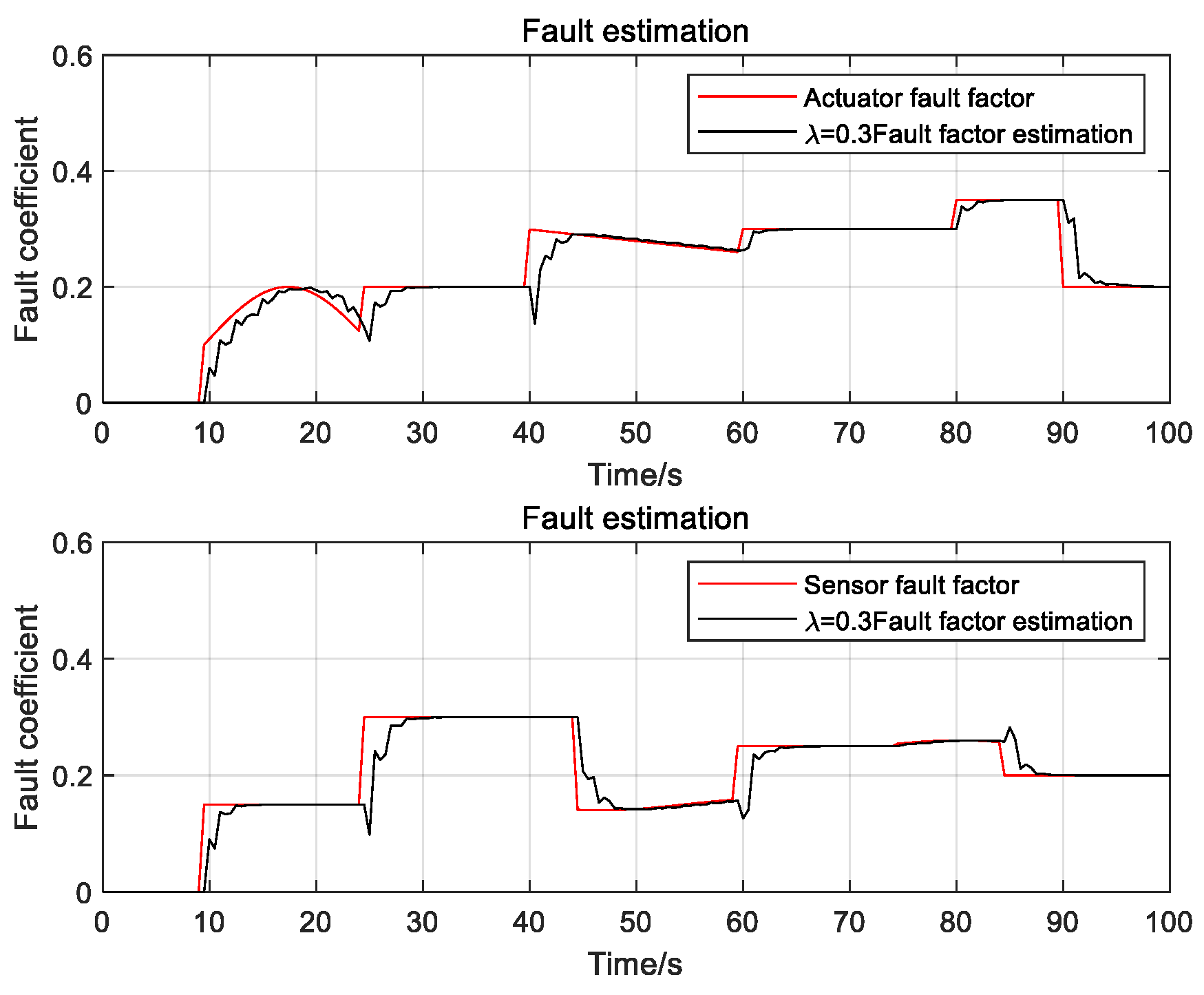
A time-varying fault is introduced:
Figure 7 shows that the DDAF-FD method can estimate time-varying faults. In addition, it can achieve simultaneous online estimation of actuator and sensor faults.
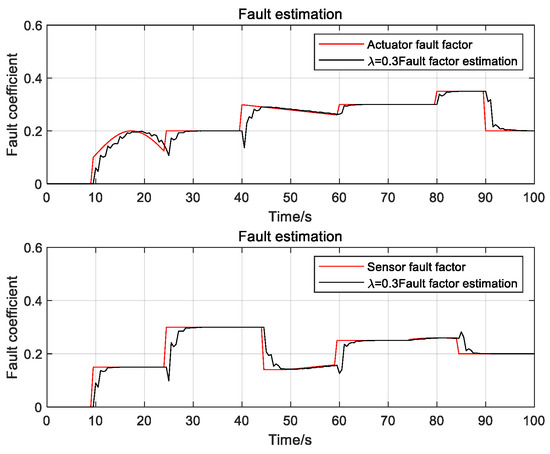
Figure 7.
Joint estimation of the actuator and sensor fault factors.
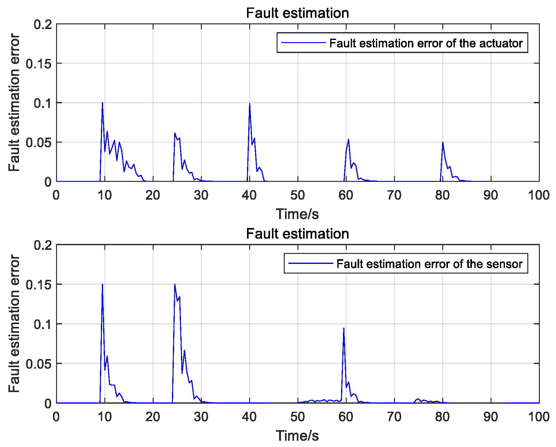
Figure 8 shows that when there are time-varying faults in the system, and when a fault changes abruptly, the fault estimation value also changes abruptly; however, the fault estimation error curve rapidly approaches zero, which implies that the DDAF-FD method can adaptively estimate time-varying faults. This proves the effectiveness of the proposed DDAF-FD algorithm.

Figure 8.
Estimation errors of the actuator and sensor fault factors.
6. Conclusions
In this paper, a data-driven method was adopted to effectively combine system parameter identification and state estimation by using only system I/O data without a system model, and a data-driven adaptive filtering method is proposed for the actuator and sensor fault diagnosis of a class of SISO nonlinear discrete systems. The simultaneous online estimation of actuator and sensor fault factors is achieved. Both the theoretical analysis via Lyapunov theory and the numerical simulation validate the effectiveness and accuracy of the proposed method. At present, there are few studies on data-driven fault diagnosis for nonlinear systems, which will be further studied in the future.
Author Contributions
Conceptualization, L.F. and H.J.; methodology, L.F.; validation, L.F., S.L. and K.G.; formal analysis, K.G.; writing—original draft preparation, K.G.; writing—review and editing, Y.W.; supervision, S.L.; project administration, L.F.; funding acquisition, L.F. All authors have read and agreed to the published version of the manuscript.
Funding
This work is supported by National Natural Science Foundation (NNSF) of China under Grant 61803036 and 61903004, Beijing Municipal Natural Science Foundation under Grant 4204098 and 4212035, North China University of Technology YuYou Talent Training Program, North China University of Technology Scientific Research Foundation, Beijing Information Science and Technology University Scientific Research Classified Development Program under Grant 2121YJPY214.
Institutional Review Board Statement
Not applicable.
Informed Consent Statement
Not applicable.
Conflicts of Interest
The author declares that there are no conflict of interest.
References
- Guo, Y.Y.; Sun, Y.C.; Li, L.B. Research on probabilistic risk assessment of aeroengine rotor failure. Proc. Inst. Mech. Eng. Part G-J. Aerosp. Eng. 2020, 234, 2337–2347. [Google Scholar] [CrossRef]
- Zhang, W.P.; Xu, D.H.; Enjeti, P.N.; Li, H.; Hawke, J.T.; Krishnamoorthy, H.S. Survey on Fault-Tolerant Techniques for Power Electronic Converters. IEEE Trans. Power Electron. 2014, 29, 6319–6331. [Google Scholar] [CrossRef]
- Volkanovski, A.; Veira, M.P. Analysis of Loss of Essential Power System Reported in Nuclear Power Plants. Sci. Technol. Nucl. Install. 2018, 2018, 3671640. [Google Scholar] [CrossRef]
- Beard, R.V. Failure accommodation in linear systems through self-reorganization. Mass. Inst. Technol. 1971, 199, 1–20. [Google Scholar]
- Mehra, R.K.; Peschon, J. An innovations approach to fault detection and diagnosis in dynamic systems. Automatica 1971, 7, 637–640. [Google Scholar] [CrossRef]
- Gao, Z.; Cecati, C.; Ding, S.X. A Survey of Fault Diagnosis and Fault-Tolerant Techniques-Part I: Fault Diagnosis with Model-Based and Signal-Based Approaches. IEEE Trans. Ind. Electron. 2015, 62, 3757–3767. [Google Scholar] [CrossRef] [Green Version]
- Gao, Z.; Cecati, C.; Ding, S.X. A Survey of Fault Diagnosis and Fault-Tolerant Techniques-Part II: Fault Diagnosis with Knowledge-Based and Hybrid/Active Approaches. IEEE Trans. Ind. Electron. 2015, 62, 3768–3774. [Google Scholar] [CrossRef]
- Safaeipour, H.; Forouzanfar, M.; Casavola, A. A survey and classification of incipient fault diagnosis approaches. J. Process. Control 2021, 97, 1–16. [Google Scholar] [CrossRef]
- Ekanayake, T.; Dewasurendra, D.; Abeyratne, S.; Ma, L.; Yarlagadda, P. Model-based fault diagnosis and prognosis of dynamic systems: A review. Procedia Manuf. 2019, 30, 435–442. [Google Scholar] [CrossRef]
- Gu, Y.; Cao, J.; Song, X.; Yao, J. A Denoising Autoencoder-Based Bearing Fault Diagnosis System for Time-Domain Vibration Signals. Wirel. Commun. Mob. Comput. 2021, 2021, 9790053. [Google Scholar] [CrossRef]
- Tariq, M.F.; Khan, A.Q.; Abid, M.; Mustafa, G. Data-Driven Robust Fault Detection and Isolation of Three-Phase Induction Motor. IEEE Trans. Ind. Electron. 2019, 66, 4707–4715. [Google Scholar] [CrossRef]
- Naderi, E.; Khorasani, K. A data-driven approach to actuator and sensor fault detection, isolation and estimation in discrete-time linear systems. Automatica 2017, 85, 165–178. [Google Scholar] [CrossRef] [Green Version]
- Gao, Z. Fault Estimation and Fault-Tolerant Control for Discrete-Time Dynamic Systems. IEEE Trans. Ind. Electron. 2015, 62, 3874–3884. [Google Scholar] [CrossRef] [Green Version]
- Ma, H.J.; Yang, G.H. Simultaneous fault diagnosis for robot manipulators with actuator and sensor faults. Inf. Sci. 2016, 366, 12–30. [Google Scholar] [CrossRef]
- Zhang, Q. Adaptive Kalman Filter for Actuator Fault Diagnosis. Automatica 2018, 93, 333–342. [Google Scholar] [CrossRef] [Green Version]
- Skriver, M.; Helck, J.; Hasan, A. Adaptive Extended Kalman Filter for Actuator Fault Diagnosis. In Proceedings of the 2019 4th International Conference on System Reliability and Safety (ICSRS), Rome, Italy, 20–22 November 2019; pp. 339–344. [Google Scholar]
- Gao, J.X.; Zhang, Q.; Chen, J.Y. EKF-Based Actuator Fault Detection and Diagnosis Method for Tilt-Rotor Unmanned Aerial Vehicles. Math. Probl. Eng. 2020, 2020, 8019017. [Google Scholar] [CrossRef]
- Gholizadeh, M.; Yazdizadeh, A.; Mohammad-Bagherpour, H. Fault detection and identification using combination of EKF and neuro-fuzzy network applied to a chemical process (CSTR). Pattern Anal. Appl. 2019, 22, 359–373. [Google Scholar] [CrossRef]
- Zhou, N.N.; He, H.W.; Liu, Z.T. UKF-based Sensor Fault Diagnosis of PMSM Drives in Electric Vehicles. In Proceedings of the 9th International Conference on Applied Energy, Jeju, Korea, 21–24 November 2017; Volume 142, pp. 2276–2283. [Google Scholar]
- Song, W.; Feng, J.; Sun, S. Data-based output tracking formation control for heterogeneous MIMO multiagent systems under switching topologies. Neurocomputing 2021, 422, 322–331. [Google Scholar] [CrossRef]
- Esmaeili, B.; Madani, S.S.; Salim, M.; Baradarannia, M.; Khanmohammadi, S. Model-free adaptive iterative learning integral terminal sliding mode control of exoskeleton robots. J. Vib. Control 2021. [Google Scholar] [CrossRef]
- Chi, R.; Hui, Y.; Zhang, S.; Huang, B.; Hou, Z. Discrete-Time Extended State Observer-Based Model-Free Adaptive Control Via Local Dynamic Linearization. IEEE Trans. Ind. Electron. 2020, 67, 8691–8701. [Google Scholar] [CrossRef]
- Hou, Z.; Jin, S. Model Free Adaptive Control: Theory and Applications; CRC Press: Boca Raton, FL, USA, 2013. [Google Scholar]
- Hou, Z.; Xiong, S. On Model-Free Adaptive Control and Its Stability Analysis. IEEE Trans. Autom. Control 2019, 64, 4555–4569. [Google Scholar] [CrossRef]
- Fan, L.; Hou, Z.; Cao, R.; Ji, H. A Novel Data-Driven Filtering Algorithm for a Class of Discrete-Time Nonlinear Systems. In Proceedings of the 2018 IEEE 7th Data Driven Control and Learning Systems Conference (DDCLS), Enshi, China, 22–27 May 2018; pp. 763–769. [Google Scholar]
- Haddad, W.M. Nonlinear Dynamical Systems and Control: A Lyapunov-Based Approach; Princeton University Press: Princeton, NJ, USA, 2008. [Google Scholar]
Publisher’s Note: MDPI stays neutral with regard to jurisdictional claims in published maps and institutional affiliations. |
© 2021 by the authors. Licensee MDPI, Basel, Switzerland. This article is an open access article distributed under the terms and conditions of the Creative Commons Attribution (CC BY) license (https://creativecommons.org/licenses/by/4.0/).