
Robust Nonlinear Control Scheme for Electro-Hydraulic Force Tracking Control with Time-Varying Output Constraint


Abstract
:1. Introduction
2. Problem Formulation and Preliminaries
3. Dos-Based TVCRC Design
3.1. DOs Design
3.2. The TVCRC Design
3.3. Stability of the Closed Loop
4. Simulation and Experimental Study
4.1. Simulation Study
- (1)
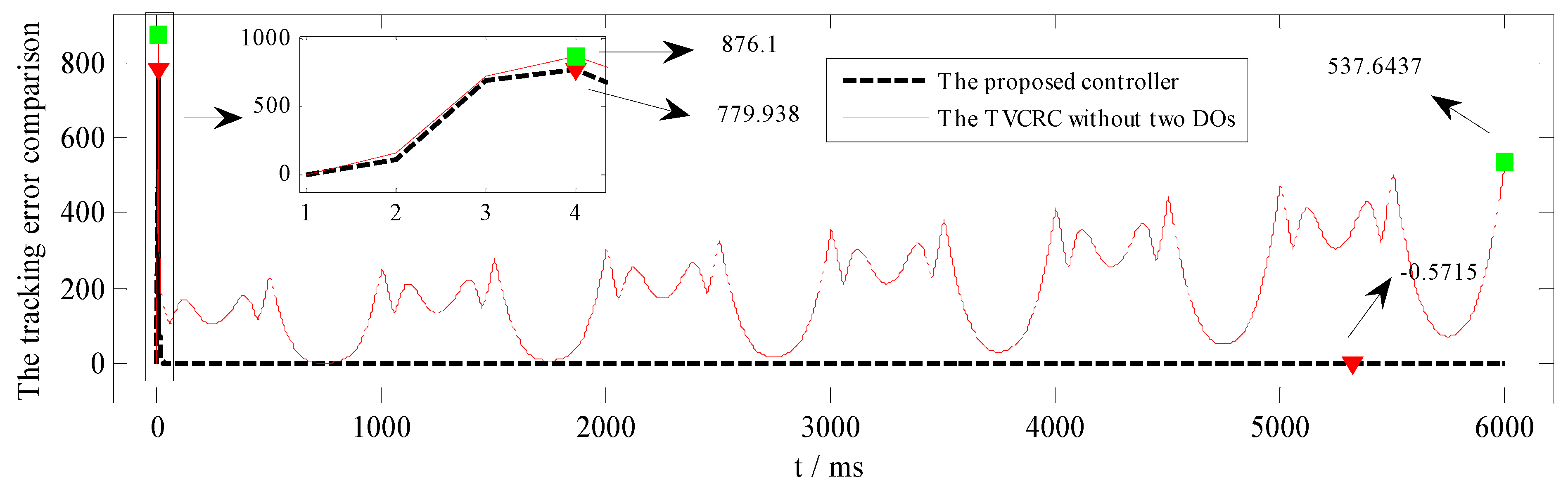
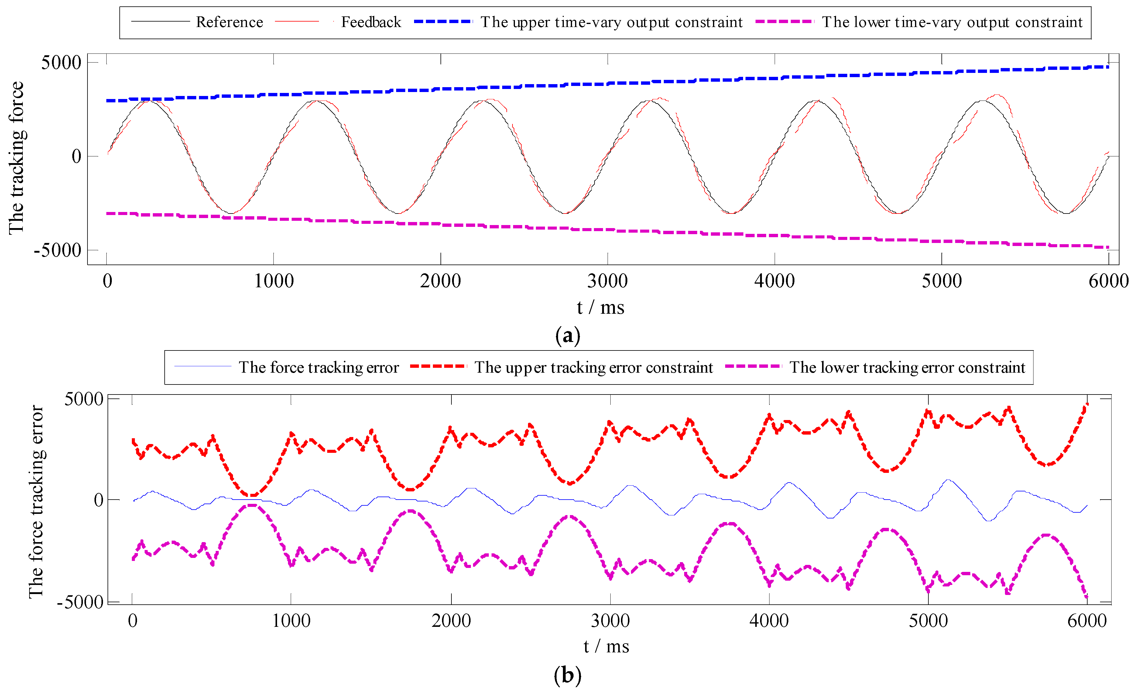
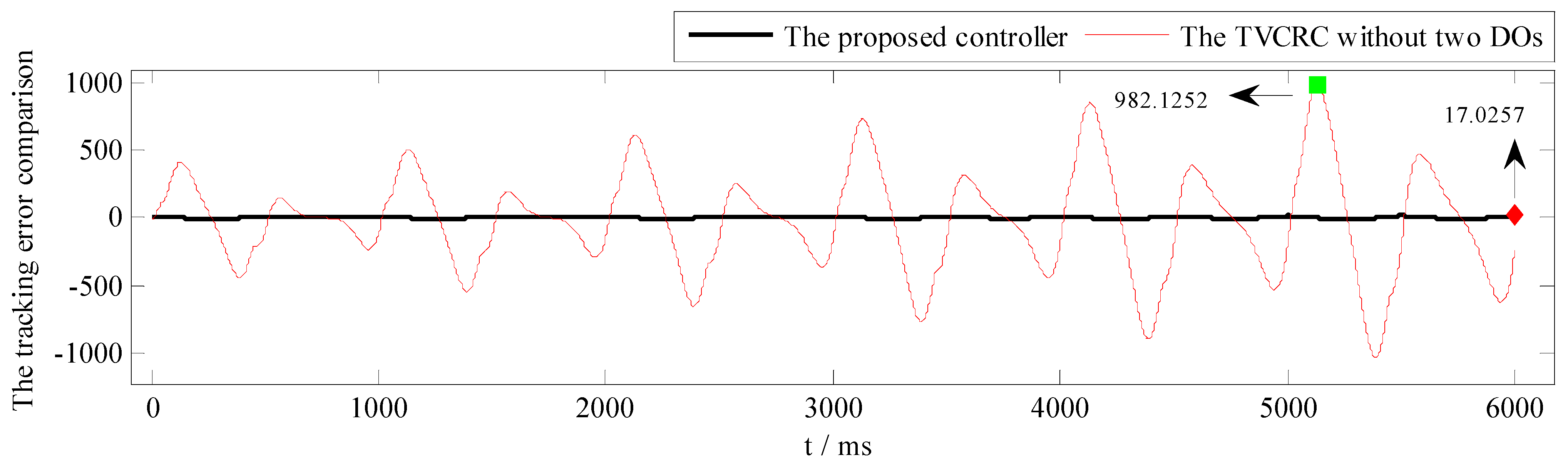
- The TVCRC without two DOs: with and , the simulation study is conducted on the software MATLAB/Simulink to validate the efficiency of the TVCRC without two DOs.
- (2)
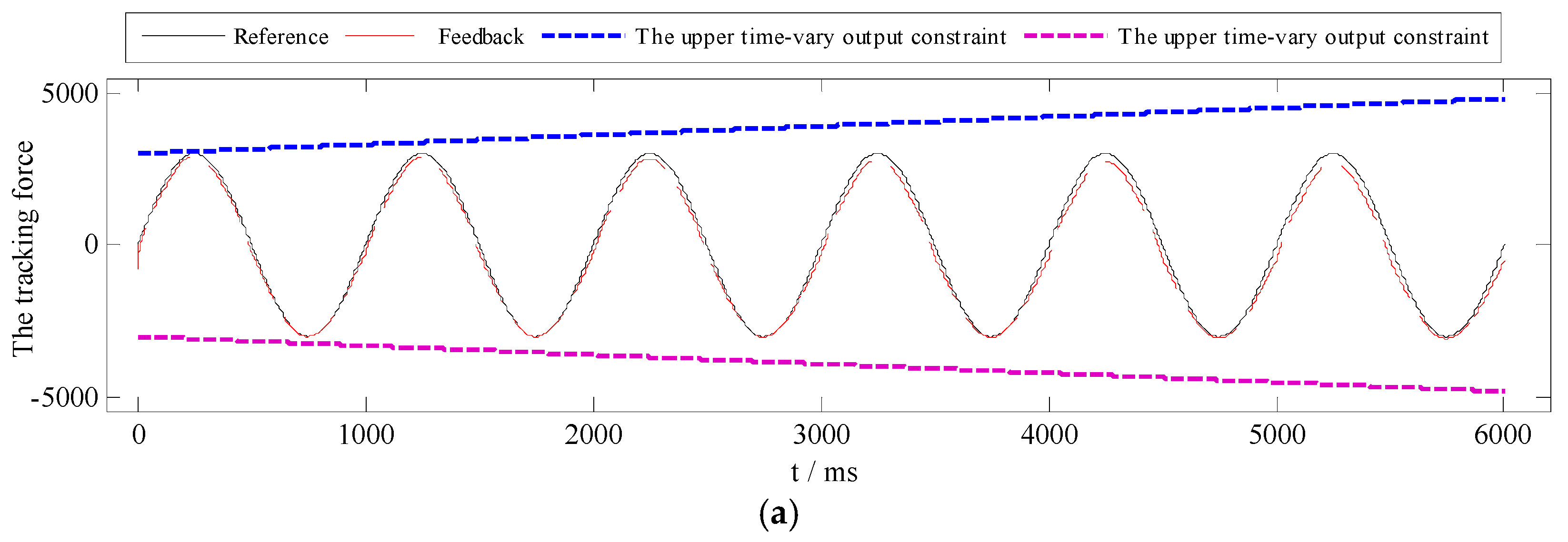
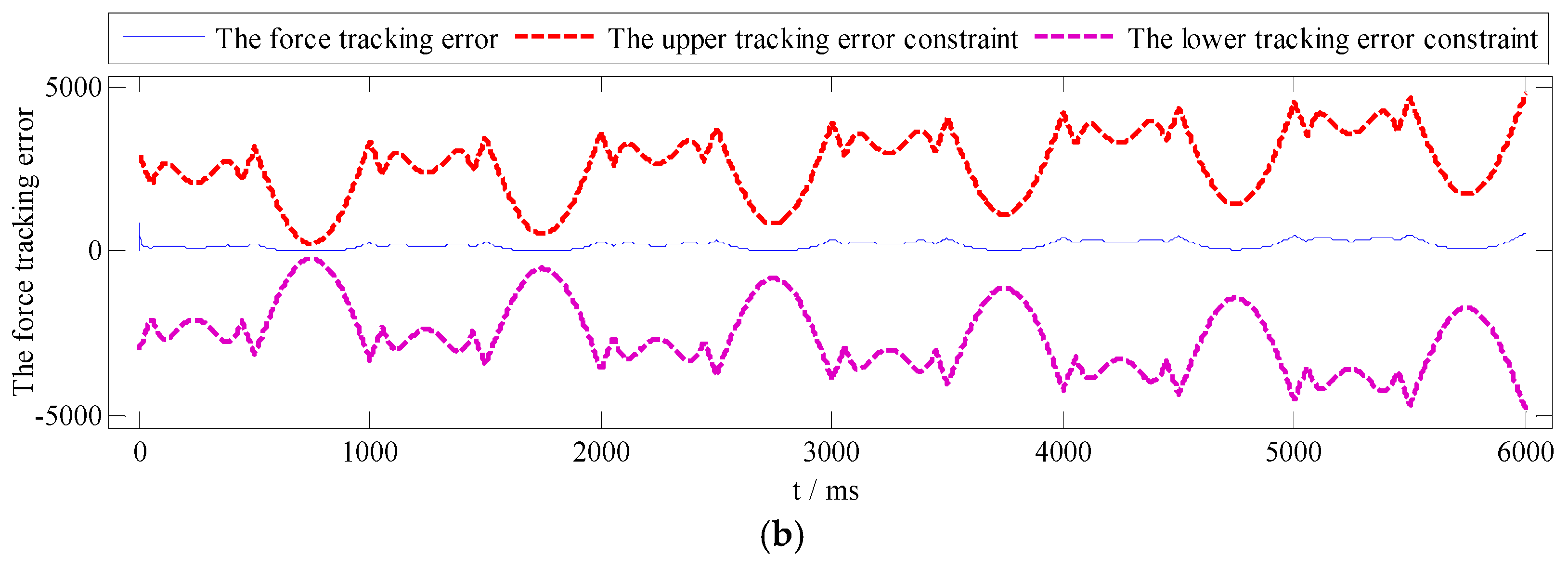
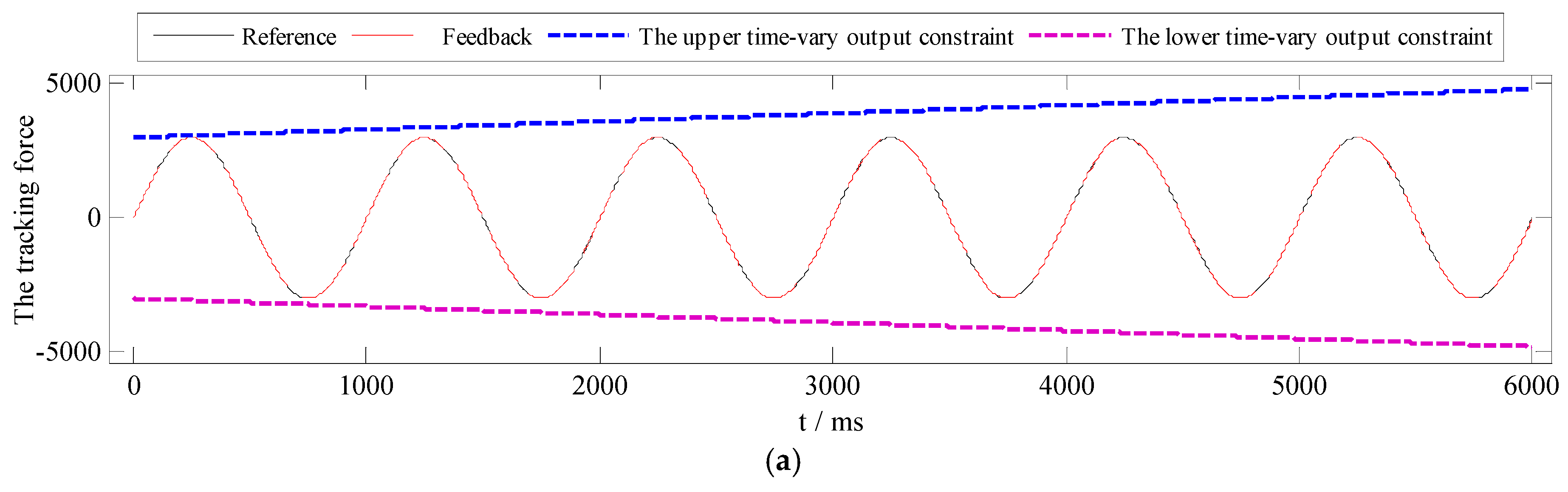
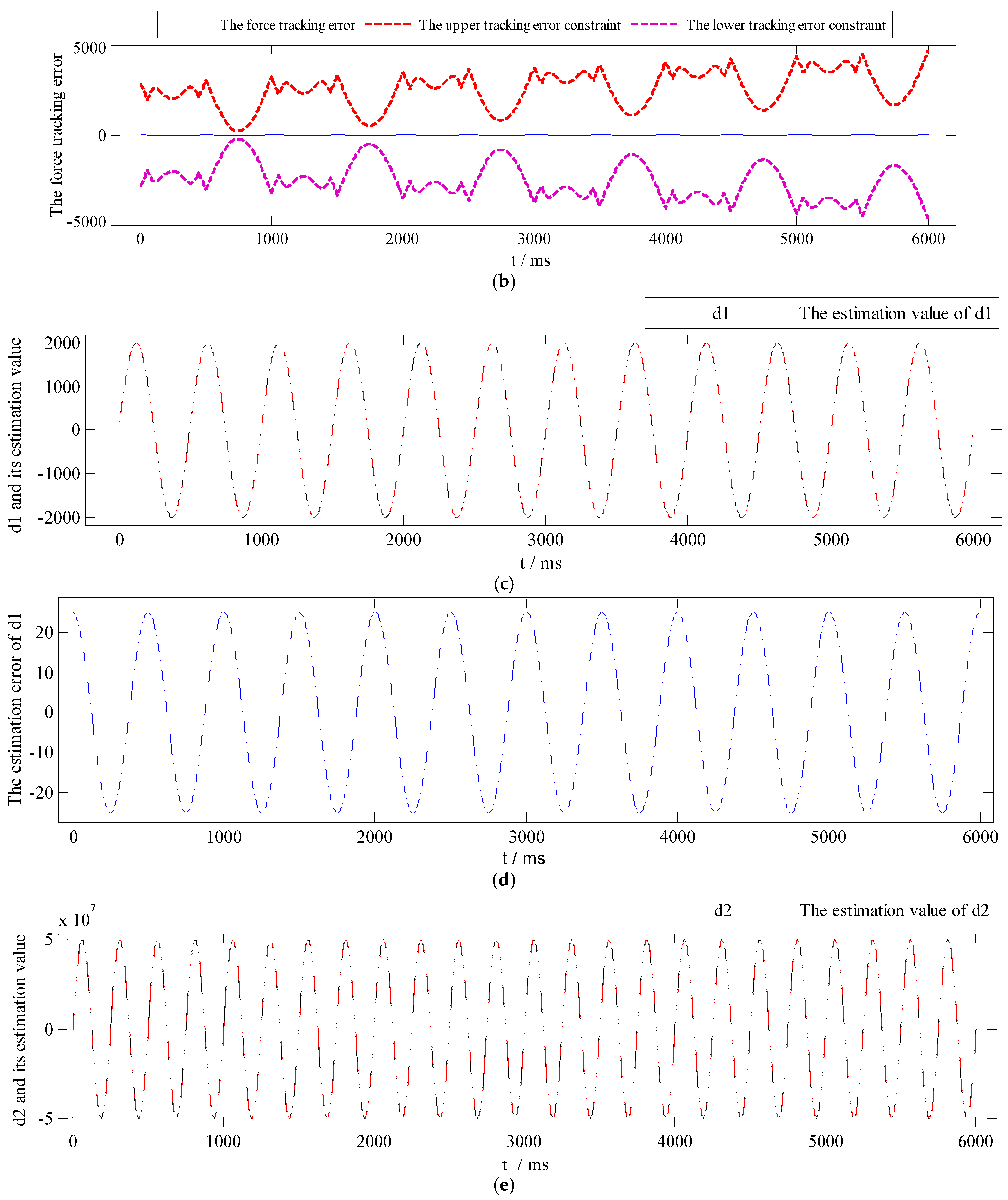
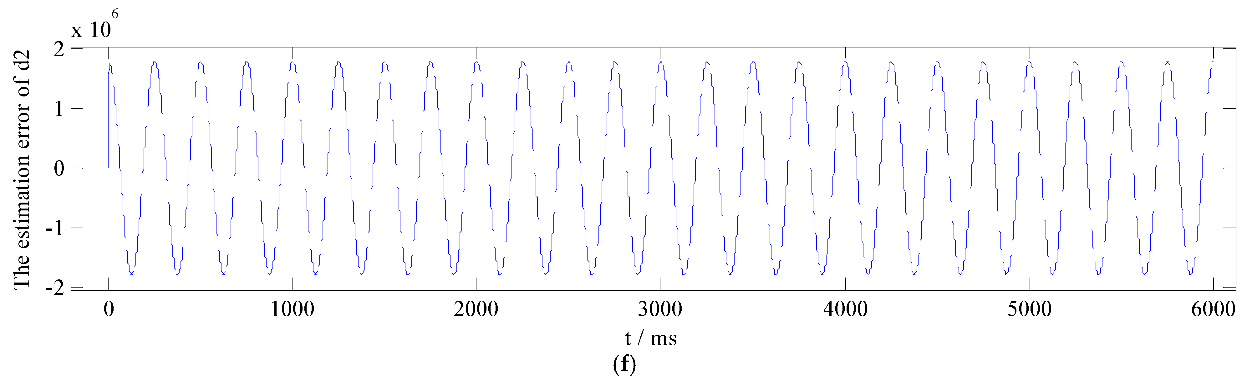
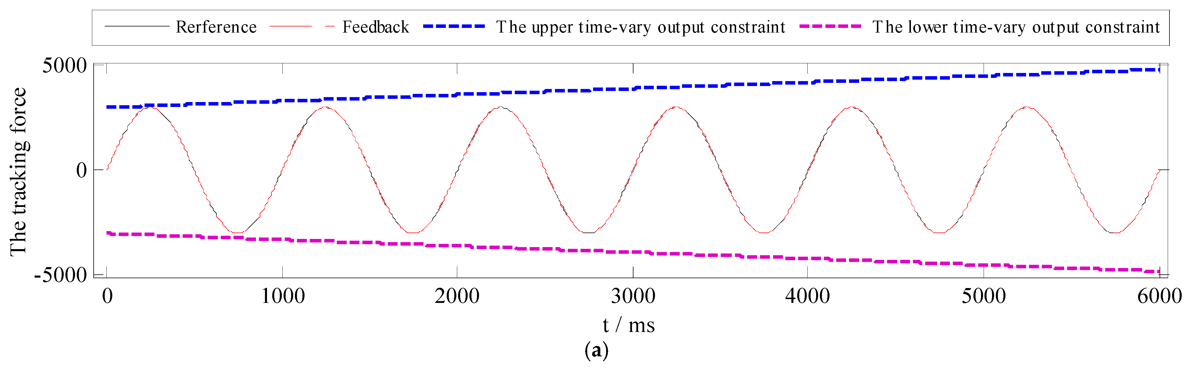
- The TVCRC with two DOs: in order to further improve the force tracking performance, two DOs based TVCRC are employed. Based on [32], the time-varying output constraint for the EHFCS can be selected as , and as a function of , is presented in Equation (57).
- (1)
- (2)
- (3)
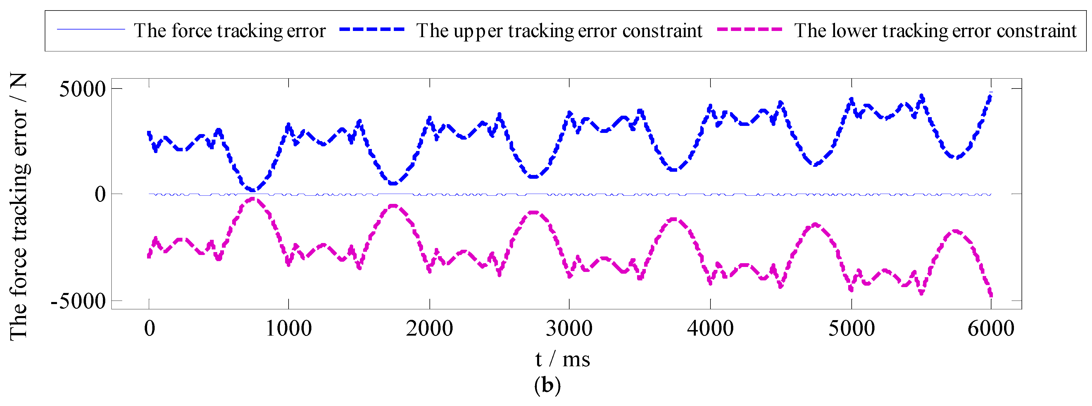
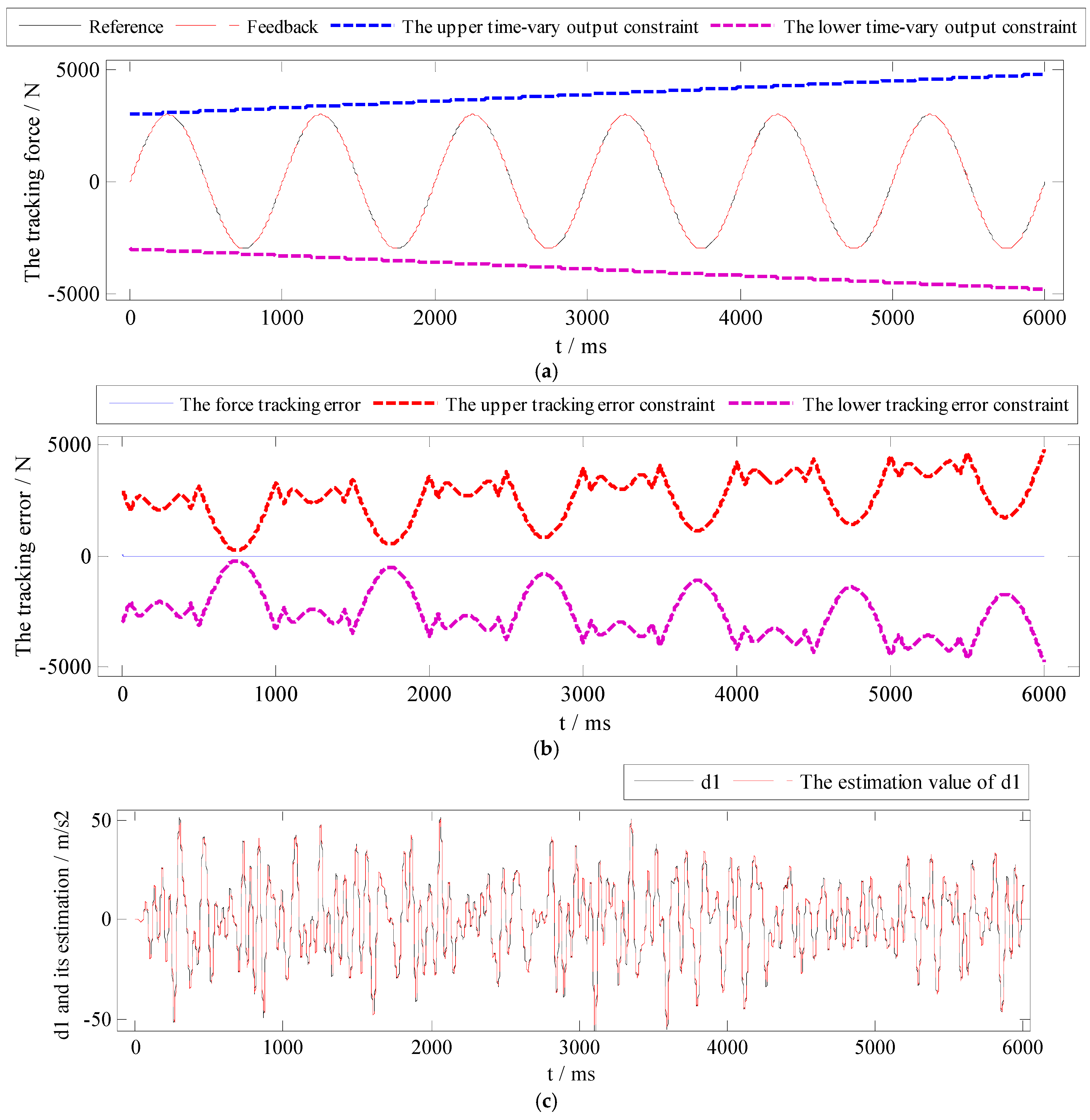
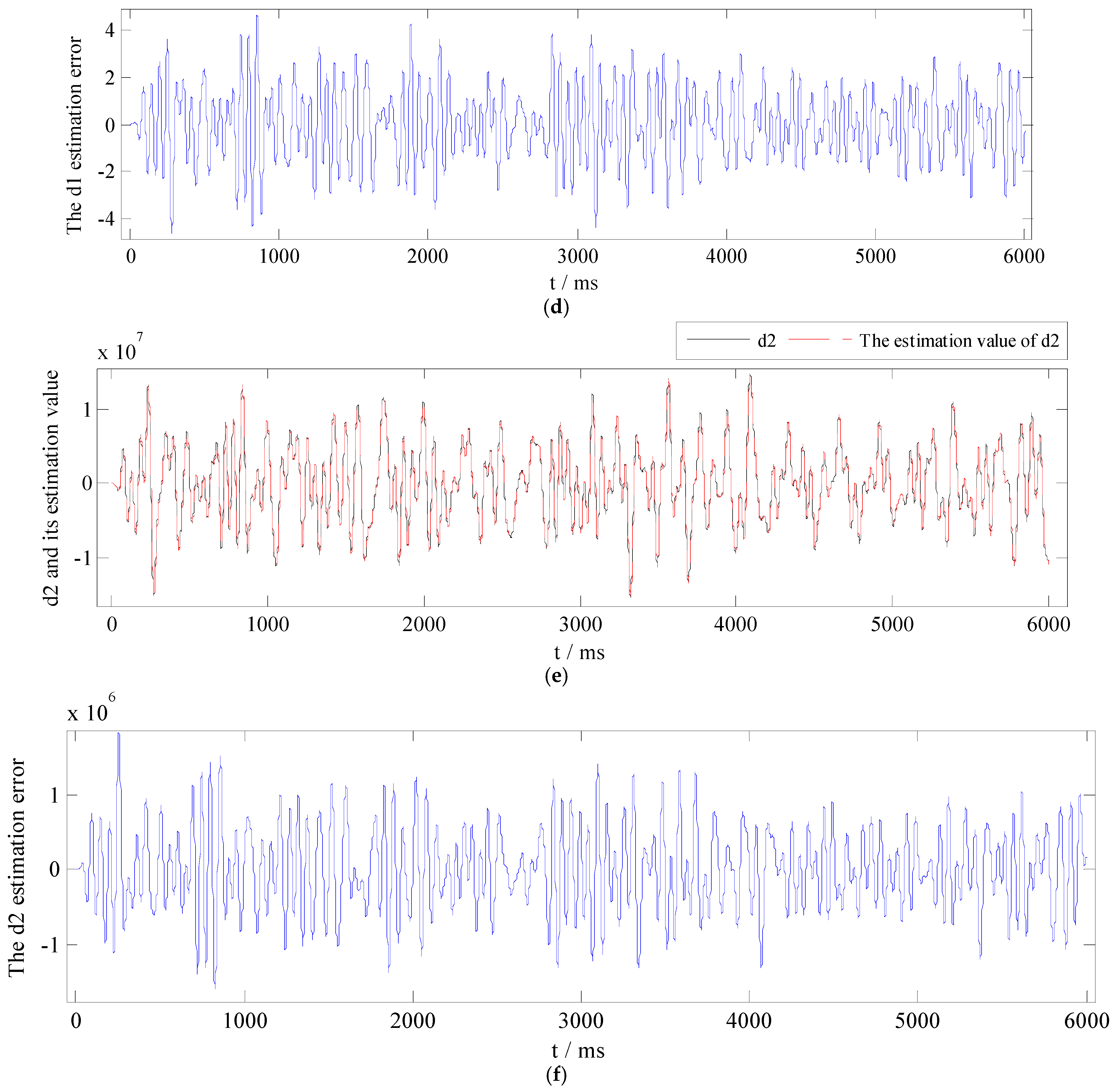
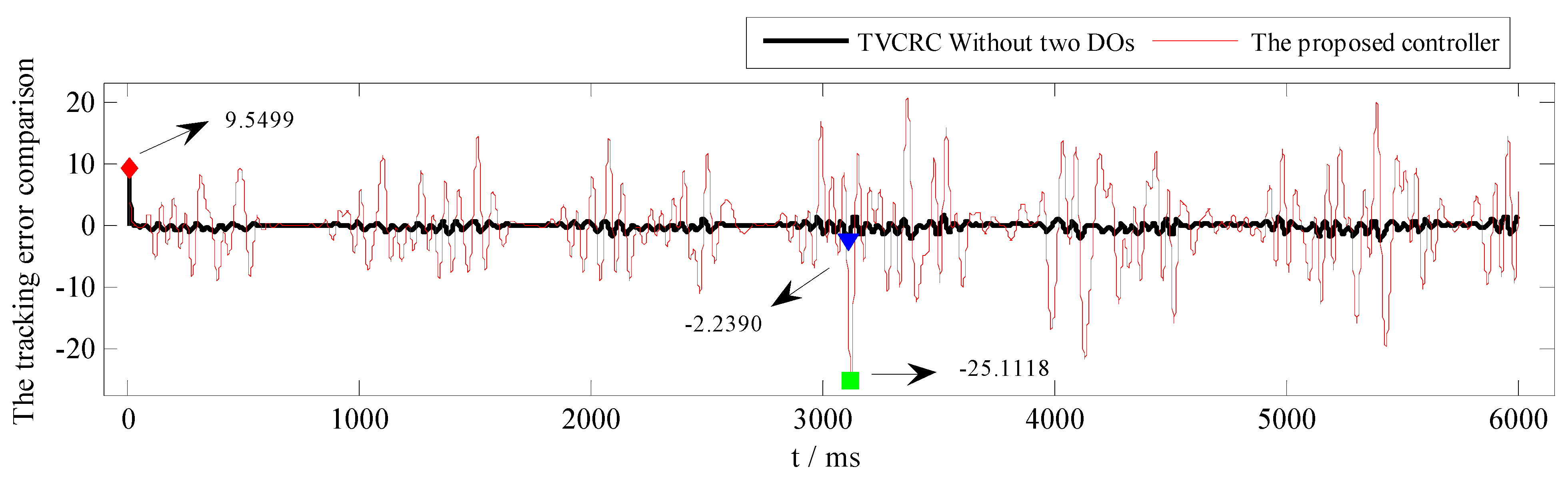
- Case 3: uniform random disturbances: d1 is a uniform random number with amplitude from −200 to 200 and a bandpass filter from 4 Hz to 20 Hz, d2 is a uniform random number with amplitude from −50,000,000 to 50,000,000 and a bandpass filter from 2 Hz to 20 Hz. The power of d1 and d2 is 373.5790 and 2.6454 × 10¹³ respectively. The simulation results are presented in Figure 9, Figure 10 and Figure 11.
- Simulation results of Case 1:
- Simulation results of Case 2:
- Simulation results of Case 3:
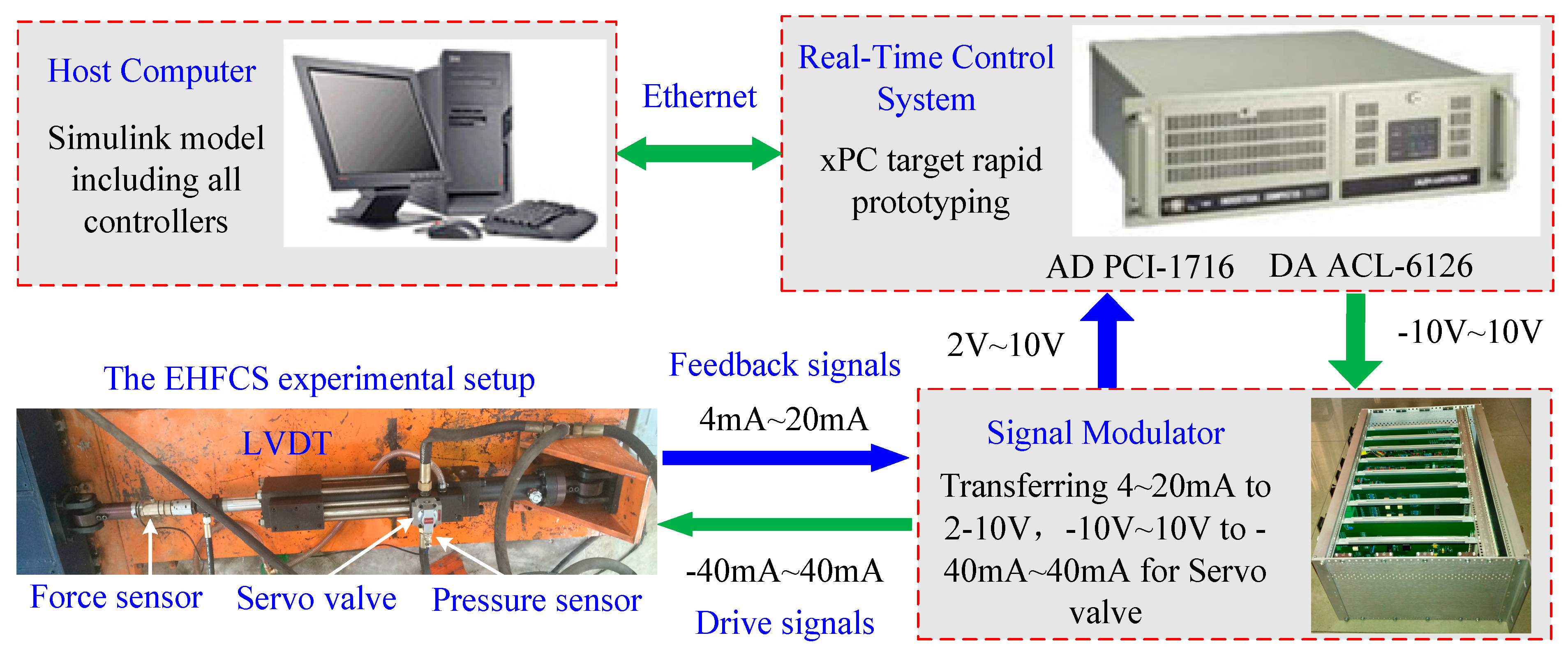
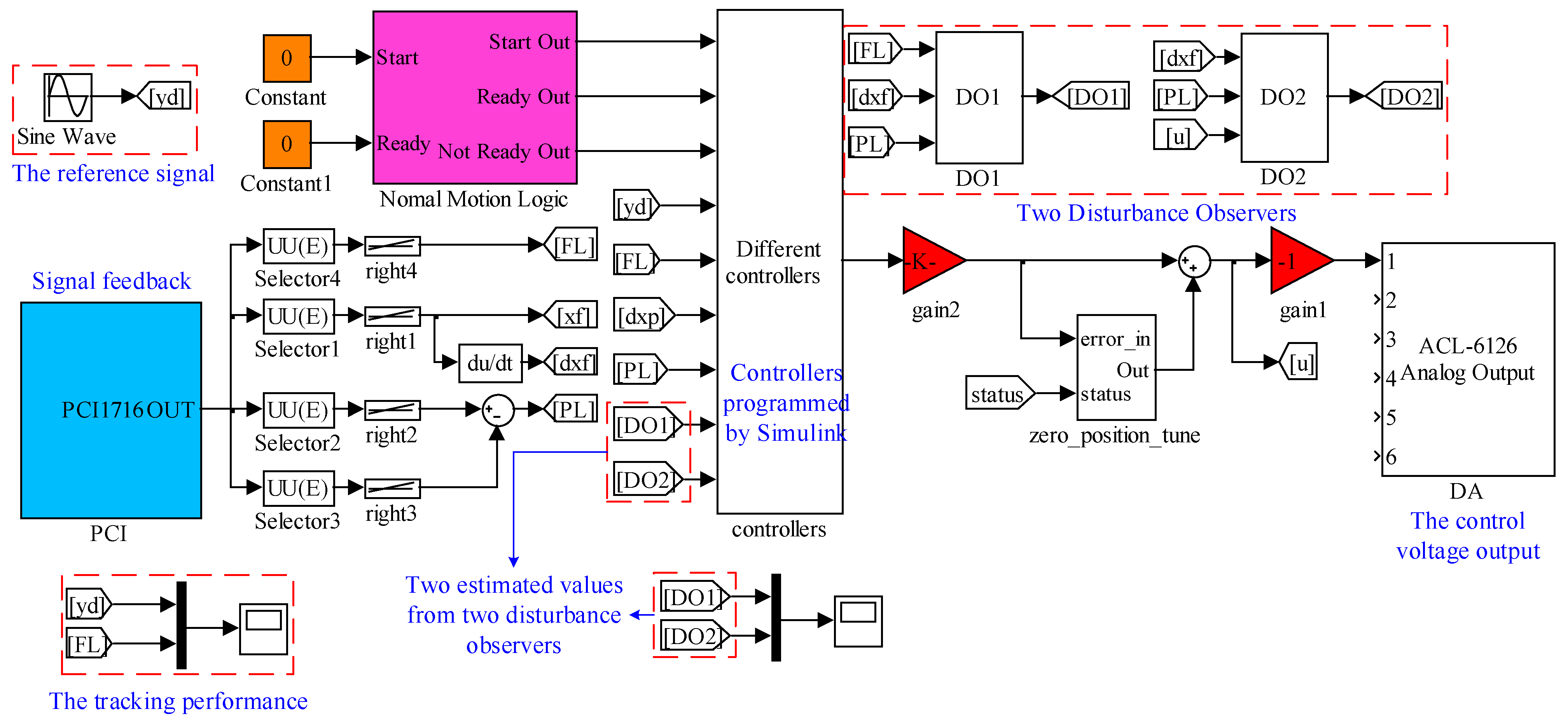
4.2. The EHFCS Experimental Setup
4.3. Comparative Experimental Results
- (1)
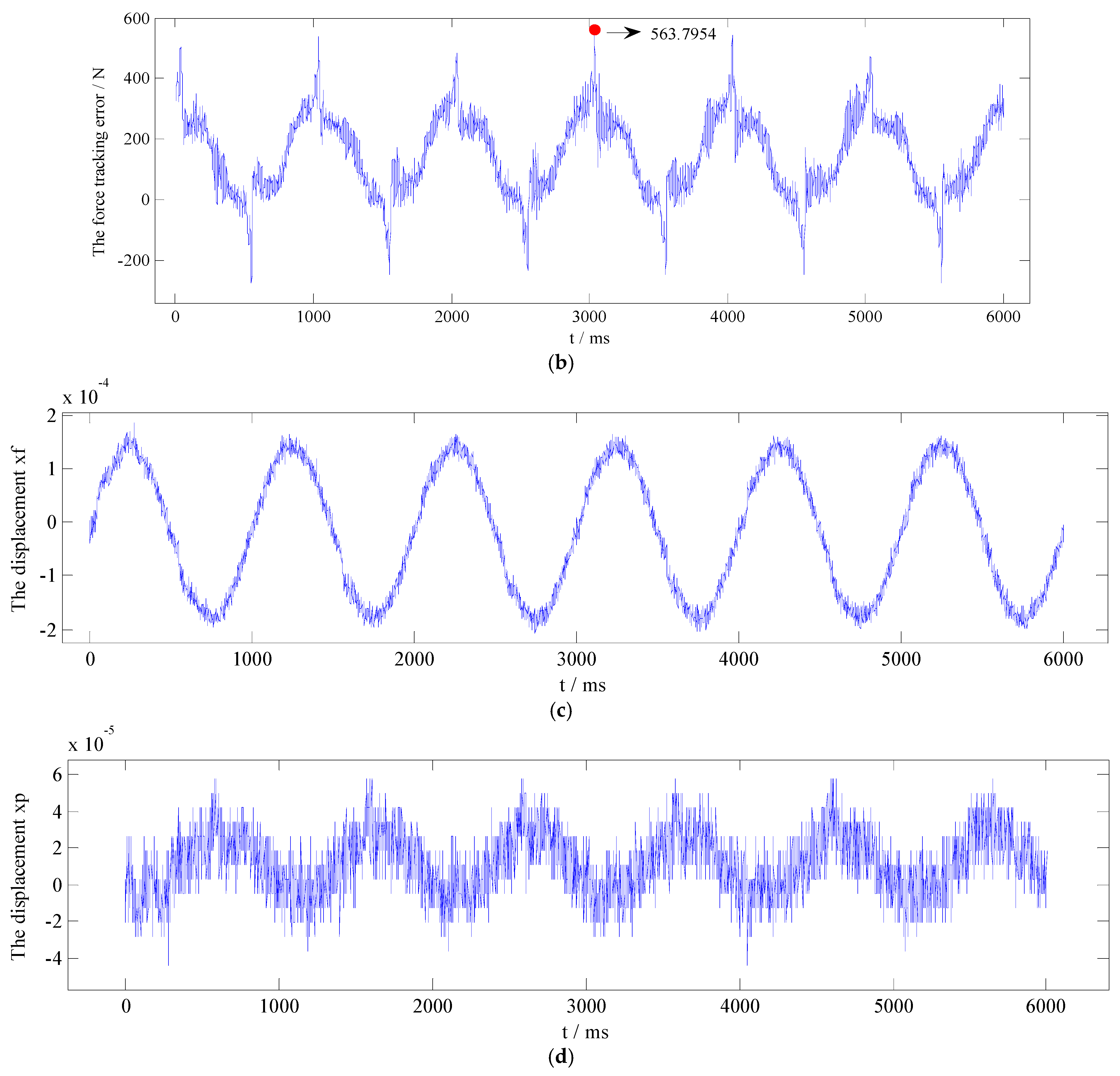
- The PI controller: the PI controller for the EHFCS can be expressed as uL = Kp*e + KIΣe. e denotes the force tracking error, uL is the control voltage. After several times tests, the tracking performance is best with control gains being selected as Kp = 0.0012 and KI = 0.03. The corresponding experimental results are shown in Figure 14;
- (2)
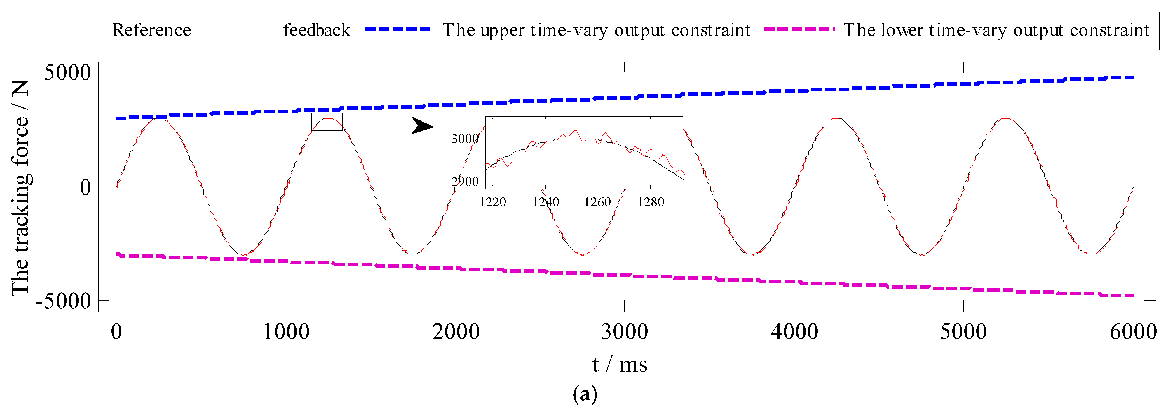
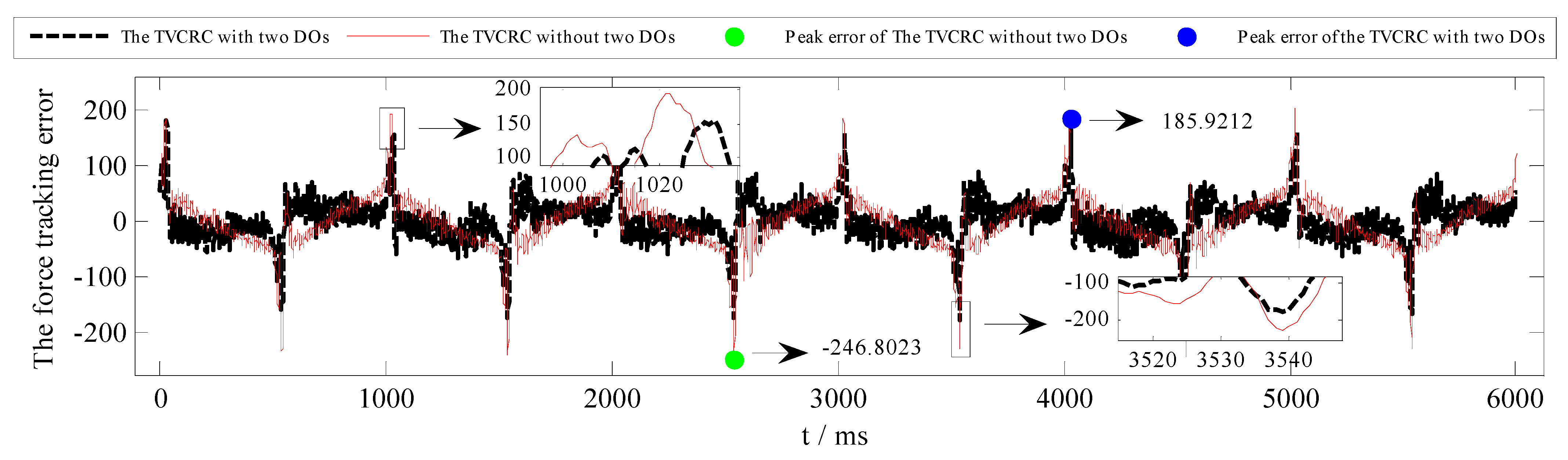
- The TVCRC without two DOs: with and , when control gains are chosen as κ1 = 420, κ2 = 421, κ3 = 365, the tracking performance are the best. The corresponding experimental results are presented in Figure 15;
- (3)
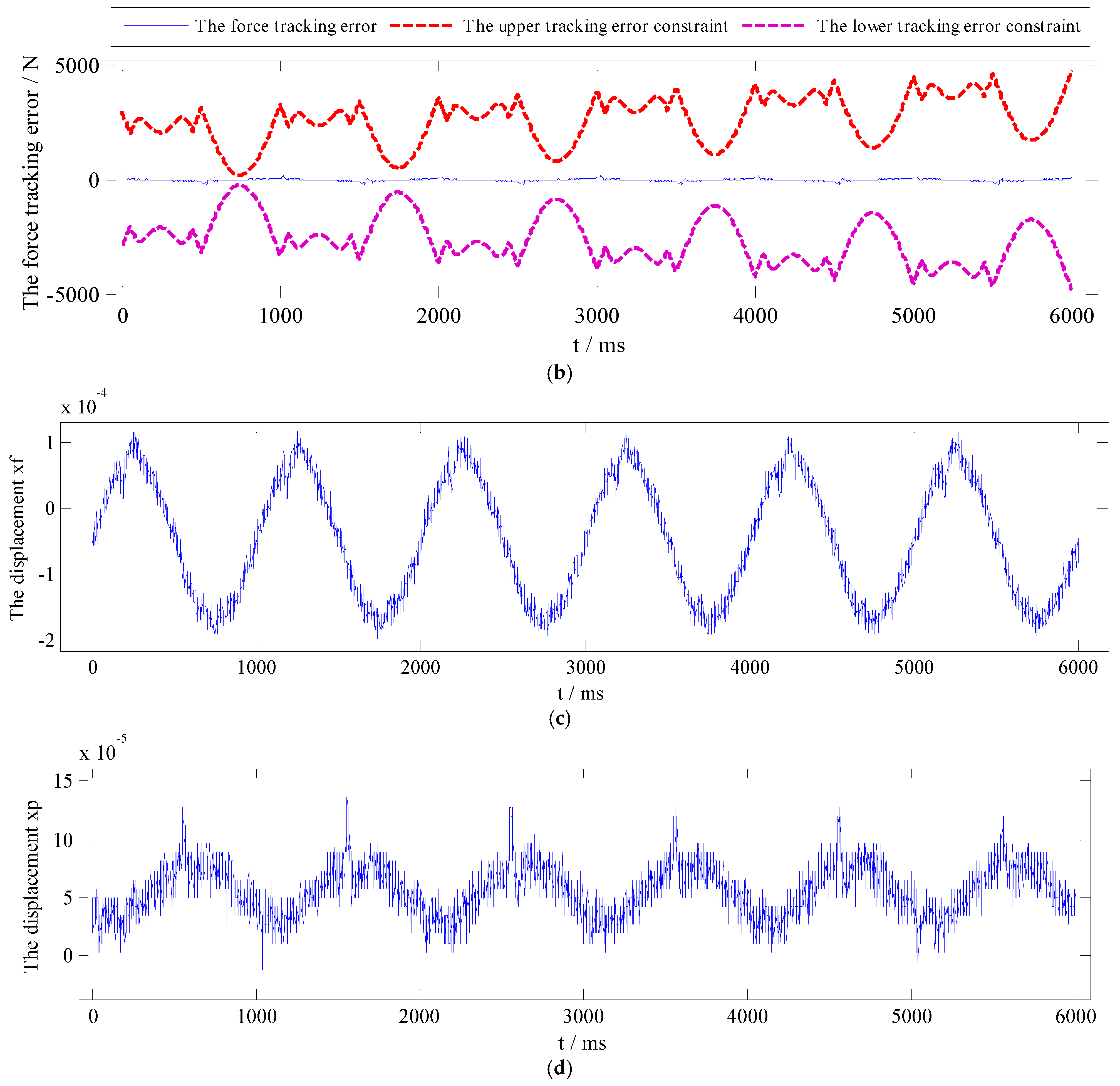
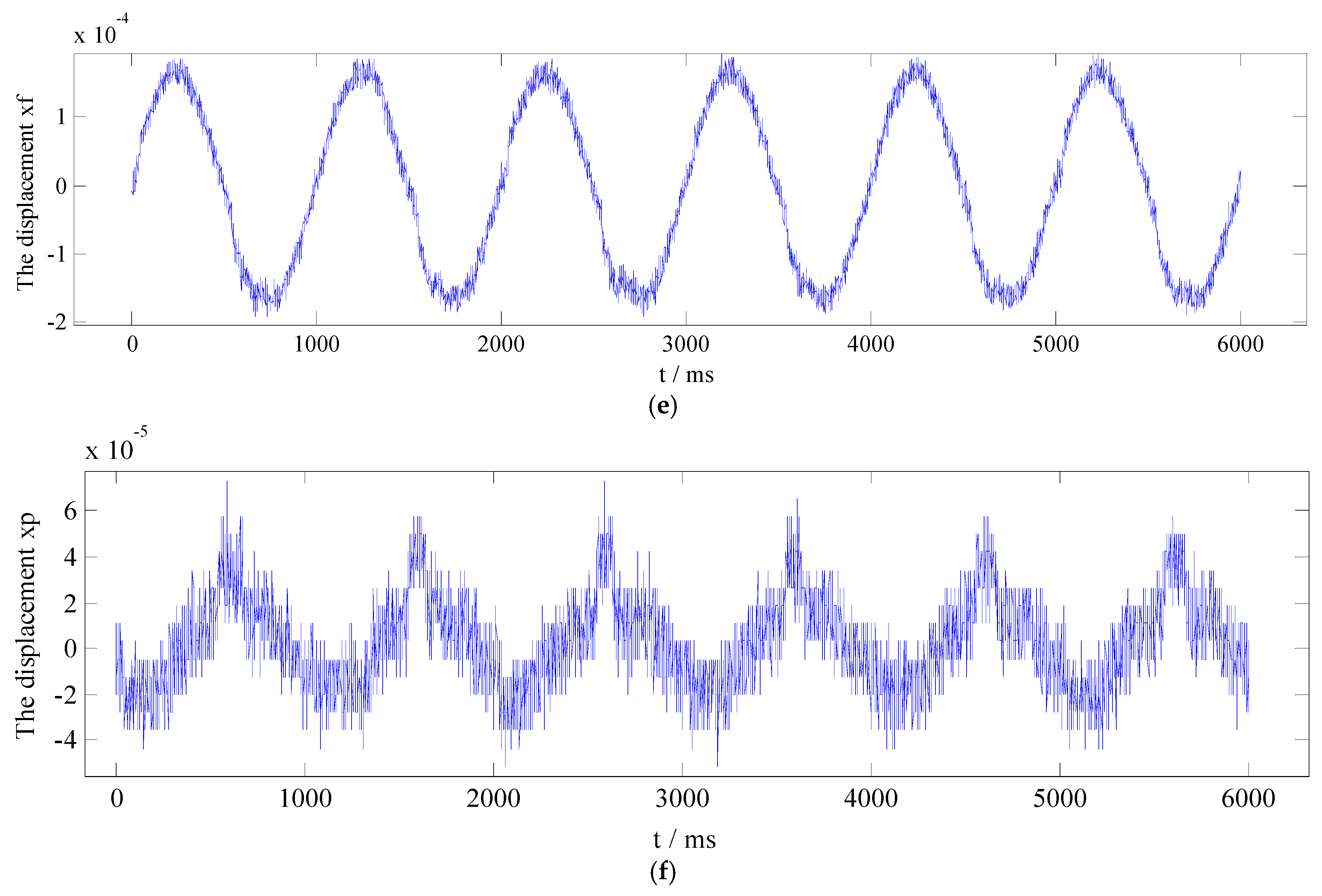
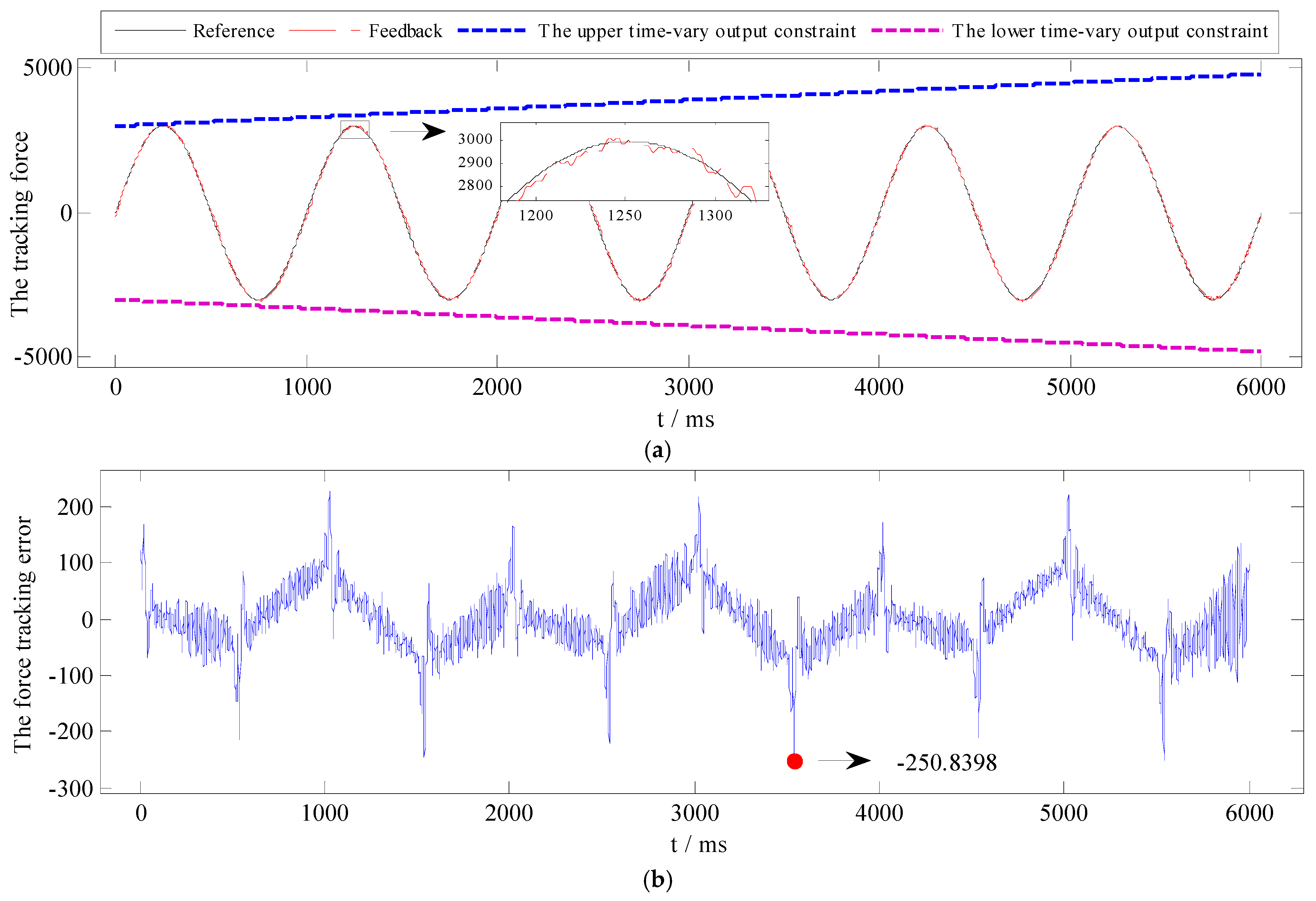
- The TVCRC with two DOs: in order to further improve the force tracking performance, the TVCRC with two DOs are employed. Control gains of two DOs and the TVCRC are selected as λ1 = 0.05, λ2 = 0.025, κ1 = 435, κ2 = 426, κ3 = 375. The performance of the TVCRC is the best among three controllers with estimated values from two DOs. The corresponding experimental results under a normal condition are presented in Figure 16. In order to further validate the robustness of the TVCRC with two DOs, a sine waves reference signal with a 0.006 m amplitude and a 0.5 Hz frequency is conducted at the position hydraulic cylinder. The corresponding experimental results under a sinusoidal position disturbance are presented in Figure 16.
5. Conclusions
- (1)
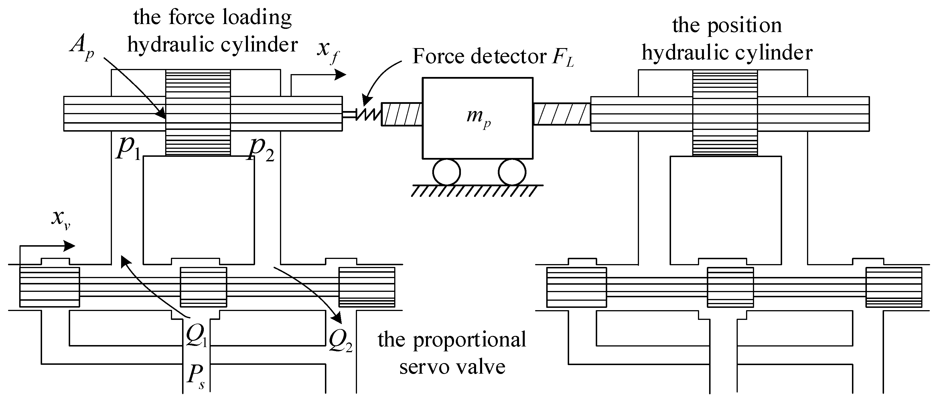
- Consider nonlinear factors like the external disturbance, parameter uncertainties as well as unmodeled characteristics in the EHFCS, the state space representation of the EHFCS is presented.
- (2)
- Based on the state representation, two DOs for the EHFCS is presented and its stability is proved by defining proper Lyapunov functions. Consequently, the TVCRC with backstepping design scheme is presented in detail.
- (3)
- Results from simulation and experimental study show that the proposed controller exhibits better performance than the TVCRC without two DOs and the conventional PI controller.
Author Contributions
Funding
Institutional Review Board Statement
Informed Consent Statement
Data Availability Statement
Conflicts of Interest
References
- Wang, C.; Quan, L.; Jiao, Z.; Zhang, S. Nonlinear adaptive control of hydraulic system with observing and compensating mismatching uncertainties. IEEE Trans. Control Syst. Technol. 2017, 26, 927–938. [Google Scholar] [CrossRef]
- Yunhua, L. Development of hybrid control of electrohydraulic torque load simulator. J. Dyn. Syst. Meas. Control Trans. ASME 2002, 124, 415–419. [Google Scholar] [CrossRef]
- Namba, R.; Yamamoto, T.; Kaneda, M. Design and experimental evaluation of a self-tuning controller supplementing a robust PID controller. JSME Int. J. Ser. C Mech. Syst. Mach. Elem. Manuf. 2001, 44, 53–60. [Google Scholar] [CrossRef] [Green Version]
- Truong, D.Q.; Ahn, K.K. Force control for hydraulic load simulator using self-tuning grey predictor-fuzzy PID. Mechatronics 2009, 19, 233–246. [Google Scholar] [CrossRef]
- Truong, D.Q.; Ahn, K.K. Parallel control for electro-hydraulic load simulator using online self tuning fuzzy PID technique. Asian J. Control 2011, 13, 522–541. [Google Scholar] [CrossRef]
- Niksefat, N.; Sepehri, N. Design and experimental evaluation of a robust force controller for an electro-hydraulic actuator via quantitative feedback theory. Control Eng. Pract. 2000, 8, 1335–1345. [Google Scholar] [CrossRef]
- Ahn, K.; Yokota, S. Design and experimental evaluation of a robust force controller for a 6-link electro-hydraulic manipulator via H∞ control theory. KSME Int. J. 2003, 17, 999–1010. [Google Scholar] [CrossRef]
- Min, L.J.; Hwan, P.S.; Shik, K.J. Design and experimental evaluation of a robust position controller for an electrohydrostatic actuator using adaptive antiwindup sliding mode scheme. Sci. World J. 2013, 2013, 590708. [Google Scholar]
- Zhao, J.; Shen, G.; Zhu, W.; Yang, C.; Yao, J. Robust force control with a feed-forward inverse model controller for electro-hydraulic control loading systems of flight simulators. Mechatronics 2016, 38, 42–53. [Google Scholar] [CrossRef]
- Dashti, Z.A.S.; Jafari, M.; Gholami, M.; Shoorehdeli, M.A. Neural—Adaptive control based on backstepping and feedback linearization for electro hydraulic servo system. In Proceedings of the 2014 Iranian Conference on Intelligent Systems (ICIS), Bam, Iran, 4–6 February 2014; IEEE: Piscataway, NJ, USA, 2014; pp. 1–6. [Google Scholar]
- Mintsa, H.A.; Venugopal, R.; Kenne, J.P.; Belleau, C. Feedback linearization-based position control of an electrohydraulic servo system with supply pressure uncertainty. IEEE Trans. Control Syst. Technol. 2012, 20, 1092–1099. [Google Scholar] [CrossRef]
- Wang, S.; Xu, Q.; Lin, R.; Yang, M.; Zheng, W.; Wang, Z. Feedback linearization control for electro-hydraulic servo system based on nonlinear disturbance observer. In Proceedings of the 2017 36th Chinese Control Conference (CCC), Dalian, China, 26–28 July 2017; IEEE: Piscataway, NJ, USA, 2017; pp. 4940–4945. [Google Scholar]
- Kaddissi, C.; Kenne, J.P.; Saad, M. Indirect adaptive control of an electrohydraulic servo system based on nonlinear backstepping. IEEE/ASME Trans. Mechatron 2011, 16, 1171–1177. [Google Scholar] [CrossRef]
- Yanada, H.; Furuta, K. Adaptive control of an electrohydraulic servo system utilizing online estimate of its natural frequency. Mechatronics 2007, 17, 337–343. [Google Scholar] [CrossRef]
- Ahn, K.K.; Nam, D.N.C.; Jin, M. Adaptive backstepping control of an electrohydraulic actuator. IEEE/ASME Trans. Mechatron. 2014, 19, 987–995. [Google Scholar] [CrossRef]
- Guo, Q.; Sun, P.; Yin, J.M.; Yu, T.; Jiang, D. Parametric adaptive estimation and backstepping control of electro-hydraulic actuator with decayed memory filter. ISA Trans. 2016, 62, 202–214. [Google Scholar] [CrossRef] [PubMed]
- Cheng, L.; Zhu, Z.C.; Shen, G.; Wang, S.; Tang, Y. Real-time force tracking control of an electro-hydraulic system using a novel robust adaptive sliding mode controller. IEEE Access 2019, 8, 13315–13328. [Google Scholar] [CrossRef]
- Yan, H.; Xu, L.L.; Dong, L.J. Finite-Time Sliding Mode Control of the Valve-Controlled Hydraulic System. In Proceedings of the 2018 10th International Conference on Modelling, Identification and Control (ICMIC), Guiyang, China, 2–4 July 2018; IEEE: Piscataway, NJ, USA, 2018; pp. 1–5. [Google Scholar]
- Chen, H.M.; Renn, J.C.; Su, J.P. Sliding mode control with varying boundary layers for an electro-hydraulic position servo system. Int. J. Adv. Manuf. Technol. 2005, 26, 117–123. [Google Scholar] [CrossRef]
- Bessa, W.M.; Dutra, M.S.; Kreuzer, E. Sliding mode control with adaptive fuzzy dead-zone compensation of an electro-hydraulic servo-system. J. Intell. Robot. Syst. 2010, 58, 3–16. [Google Scholar] [CrossRef]
- Yao, J.; Jiao, Z.; Ma, D. Extended-state-observer-based output feedback nonlinear robust control of hydraulic systems with backstepping. IEEE Trans. Ind. Electron. 2014, 61, 6285–6293. [Google Scholar] [CrossRef]
- Tri, N.M.; Nam, D.N.C.; Park, H.G.; Ahn, K.K. Trajectory control of an electro-hydraulic actuator using an iterative backstepping control scheme. Mechatronics 2015, 29, 96–102. [Google Scholar] [CrossRef]
- Guo, Q.; Zhang, Y.; Celler, B.G.; Su, S.W. Backstepping control of electro-hydraulic system based on extended-state-observer with plant dynamics largely unknown. IEEE Trans. Ind. Electron. 2016, 63, 6909–6920. [Google Scholar] [CrossRef]
- Won, D.; Kim, W.; Shin, D.; Chung, C.C. High-gain disturbance observer-based backstepping control with output tracking error constraint for electro-hydraulic systems. IEEE Trans. Control Syst. Technol. 2014, 23, 787–795. [Google Scholar] [CrossRef]
- Seo, J.H.; Shim, H.; Back, J. Consensus of high-order linear systems using dynamic output feedback compensator: Low gain approach. Automatica 2009, 45, 2659–2664. [Google Scholar] [CrossRef]
- Tee, K.P.; Ge, S.S.; Tay, E.H. Barrier Lyapunov functions for the control of output-constrained nonlinear systems. Automatica 2009, 45, 918–927. [Google Scholar] [CrossRef]
- Liu, Y.J.; Tong, S. Barrier Lyapunov functions-based adaptive control for a class of nonlinear pure-feedback systems with full state constraints. Automatica 2016, 64, 70–75. [Google Scholar] [CrossRef]
- Cao, F.; Liu, J. Vibration control for a rigid-flexible manipulator with full state constraints via Barrier Lyapunov Function. J. Sound Vib. 2017, 406, 237–252. [Google Scholar] [CrossRef]
- Niu, B.; Zhao, J. Barrier Lyapunov functions for the output tracking control of constrained nonlinear switched systems. Syst. Control Lett. 2013, 62, 963–971. [Google Scholar] [CrossRef]
- Zhang, J. Integral barrier Lyapunov functions-based neural control for strict-feedback nonlinear systems with multi-constraint. Int. J. Control Autom. Syst. 2018, 16, 2002–2010. [Google Scholar] [CrossRef]
- Tee, K.P.; Ren, B.; Ge, S.S. Control of nonlinear systems with time-varying output constraints. Automatica 2011, 47, 2511–2516. [Google Scholar] [CrossRef]
- Yang, G. Dual extended state observer-based backstepping control of electro-hydraulic servo systems with time-varying output constraints. Trans. Inst. Meas. Control 2020, 42, 1070–1080. [Google Scholar] [CrossRef]
- Liu, Y.J.; Lu, S.; Tong, S. Neural network controller design for an uncertain robot with time-varying output constraint. IEEE Trans. Syst. Man Cybern. Syst. 2016, 47, 2060–2068. [Google Scholar] [CrossRef]


| Parameters | Values | Parameters | Values |
|---|---|---|---|
| Ap | 1.88 × 10⁻³ m2 | mp | 500 kg |
| βe | 6.9 × 10⁸ Pa | Vt | 0.38 × 10⁻³ m3 |
| △Pr | 6 × 10⁶ Pa | umax | 10 V |
| Ps | 8 × 10⁶ Pa | Qr | 38 L/min |
| Bp | 7500 N/(m/s) | Ctl | 4.6 × 10⁻¹⁷ m3/s/Pa |
| Controllers | The PE/N | The RMSE/N |
|---|---|---|
| In the Case 1 simulation study | ||
| The TVCRC without two DOs | 876.1 | 225.39 |
| The TVCRC with two DOs | 779.938 | 15.8003 |
| In the Case 2 simulation study | ||
| The TVCRC without two DOs | 982.1252 | 375.4193 |
| The TVCRC with two DOs | 17.0257 | 5.2238 |
| In the Case 3 simulation study | ||
| The TVCRC without two DOs | 25.1118 | 5.8018 |
| The TVCRC with two DOs | 9.5499 | 0.6556 |
| Hardware | Quantity | Type |
|---|---|---|
| The servo valve | 2 | G762/Moog |
| PCI-1716 | 1 | Advantech |
| ACL-6126 | 1 | Linghua |
| The displacement sensor | 1 | 18 Series/Germanjet |
| The pressure sensor | 2 | NS-P-I/Tianmu |
| The force detector | 1 | NS-WL2/Tianmu |
| Controllers | The PE/N | The RMSE/N |
|---|---|---|
| The PI controller | 563.7953 | 198.1104 |
| The TVCRC without two DOs | 246.8023 | 47.9127 |
| The TVCRC with two DOs | 185.9212 | 36.7162 |
| Controllers | The PE/N | The RMSE/N |
|---|---|---|
| The TVCRC with two DOs under a sinusoidal position disturbance | 250.8398 | 56.6911 |
Publisher’s Note: MDPI stays neutral with regard to jurisdictional claims in published maps and institutional affiliations. |
© 2021 by the authors. Licensee MDPI, Basel, Switzerland. This article is an open access article distributed under the terms and conditions of the Creative Commons Attribution (CC BY) license (https://creativecommons.org/licenses/by/4.0/).
Share and Cite
Zang, W.; Zhang, Q.; Su, J.; Feng, L. Robust Nonlinear Control Scheme for Electro-Hydraulic Force Tracking Control with Time-Varying Output Constraint. Symmetry 2021, 13, 2074. https://doi.org/10.3390/sym13112074
Zang W, Zhang Q, Su J, Feng L. Robust Nonlinear Control Scheme for Electro-Hydraulic Force Tracking Control with Time-Varying Output Constraint. Symmetry. 2021; 13(11):2074. https://doi.org/10.3390/sym13112074
Chicago/Turabian StyleZang, Wanshun, Qiang Zhang, Jinpeng Su, and Long Feng. 2021. "Robust Nonlinear Control Scheme for Electro-Hydraulic Force Tracking Control with Time-Varying Output Constraint" Symmetry 13, no. 11: 2074. https://doi.org/10.3390/sym13112074