Machine Learning for Conservative-to-Primitive in Relativistic Hydrodynamics

Abstract

The numerical solution of relativistic hydrodynamics equations in conservative form requires root-finding algorithms that invert the conservative-to-primitive variables map. These algorithms employ the equation of state of the fluid and can be computationally demanding for applications involving sophisticated microphysics models, such as those required to calculate accurate gravitational wave signals in numerical relativity simulations of binary neutron stars. This work explores the use of machine learning methods to speed up the recovery of primitives in relativistic hydrodynamics. Artificial neural networks are trained to replace either the interpolations of a tabulated equation of state or directly the conservative-to-primitive map. The application of these neural networks to simple benchmark problems shows that both approaches improve over traditional root finders with tabular equation-of-state and multi-dimensional interpolations. In particular, the neural networks for the conservative-to-primitive map accelerate the variable recovery by more than an order of magnitude over standard methods while maintaining accuracy. Neural networks are thus an interesting option to improve the speed and robustness of relativistic hydrodynamics algorithms.

1. Introduction

Relativistic hydrodynamics is often written as a set of conservation laws (with source terms)

$$\frac{\partial \mathbf{u}}{\partial t}+\frac{\partial {\mathbf{F}}^i(\mathbf{u})}{\partial x^i}=\mathbf{s},$$

(1)

where the state vector $\mathbf{u}=\left(D,S_i,\tau \right)$ is composed of the conserved variables: rest-mass density, momentum density and the energy density relative to D, $\tau :=E-D$, all measured in the laboratory frame [1] ($i=1,2,3$) (we focus here on Cartesian coordinates and special relativity, although the main results of the paper are directly applicable to arbitrary coordinate system and general relativistic hydrodynamics). Conserved variables are related to primitive variables, $\mathbf{w}=\left(\rho ,v^i,ϵ,p\right)$, defined in the local rest frame of the fluid through (in units of light speed $c=1$)

$$D=\rho W,S_i=\rho h{W}^2{v}_i,\tau =\rho h{W}^2-p-D,$$

(2)

where $\rho$ is the rest-mass density, $v^i$ the fluid’s 3-velocity, $ϵ$ the specific internal energy (the total energy is $e=\rho (1+ϵ)$), p is the pressure, $h=1+ϵ+p/\rho$ is the specific enthalpy and $W={(1-v^2)}^{-1/2}$ is the Lorentz factor between the two reference frames. ${\mathbf{F}}^i=(D{v}^i,S^1{v}^i+p{\delta }^{1i},S^2{v}^i+p{\delta }^{2i},S^3{v}^i+p{\delta }^{3i},S^i-D{v}^i)$ are the flux vectors. The conservative-to-primitive transformation $\mathbf{w}(\mathbf{u})$ inverting (2) cannot be written in closed form. The system (1) is closed with an equation of state (EOS). In its simplest form, the EOS is the thermodynamical relation connecting the pressure to the fluid’s rest-mass density and internal energy, $p=\overline{p}(\rho ,ϵ)$. If more particle species are considered, then the EOS also includes additional thermodynamical potentials. For example, the Helmholtz and Lattimer–Swesty EOS used in various relativistic astrophysics simulations [2,3] return the pressure as function of the rest-mass density (or baryon number density), the temperature and the electron fraction, i.e., $p=\overline{p}(\rho ,T,Y_e)$. In this case, Equation (1) can also contain additional continuity equations for the rest-mass or number densities of the different species (e.g., for the variable $D{Y}_e$). For a causal EOS, the system (1) is hyperbolic [4]. The conservative form of the equations allows the application of robust mesh-based numerical methods that correctly capture weak solutions, e.g., shocks [5,6]. In an astrophysical context, these high-resolution shock-capturing (HRSC) methods are routinely employed for the simulation of relativistic jets [1,7], supernova explosions [8] and binary neutron star mergers in general relativity [9,10,11].

A central algorithmic step in hydrodynamics codes is the computation of the conservative-to-primitive (C2P) inversion. This calculation is performed by applying root finders at each mesh point and for each r.h.s. evaluation during the time evolution and it involves an evaluation of the EOS. In multi-dimensional simulations including microphysics, this procedure can become cumbersome and can lead to numerical errors and failures, see e.g., discussions in [12,13,14]. For example, general relativistic simulation of neutron star mergers with microphysics typically employ a C2P procedure composed of two nested root finders (Newton–Raphson algorithms) during which 3D interpolations of EOS tables are performed to find the searched-for variable (e.g., the pressure $\overline{p}(\rho ,T,Y_e)$), e.g., [15,16,17]. This procedure is called at each grid point for each time subcycle, resulting in more than ${10}^9$ calls per millisecond of evolution in simulations that currently span up to hundreds of milliseconds [17,18,19]. The computational cost of the C2P amounts up to ∼18% of the total cost for computing the r.h.s. of general relativistic equations in hyperbolic form. The C2P also impacts parallel computations and produces load imbalances since different mesh points (ranks) require different workloads. Moreover, the C2P computation is memory intensive as about 300 MB of EOS data must be loaded for these operations. A key goal of numerical relativity is to use such simulations to generate highly accurate gravitational wave signals. These are used to detect binary neutron star mergers in gravitational wave detectors such as the Laser Interferometer Gravitational Wave Observatory (LIGO) and then to perform parameter estimation to extract the parameters of the neutron stars from the wave signal. Improving the performance of simulations such as those detailed above will allow numerical relativity codes to generate more accurate gravitational waveforms more efficiently.

This paper explores a new approach to the conservative-to-primitive inversion based on supervised learning. Specifically, the use of artificial neural networks is investigated in order to produce fast algorithms that can substitute either a multi-dimensional EOS interpolation or the entire transformation of variables without affecting the accuracy of the solution. Section 2 summarizes the construction of simple neural networks for the EOS and the C2P adopting an analytical $\mathsf{\Gamma }$-law EOS as a benchmark,

$$\overline{p}(\rho ,ϵ)=(\mathsf{\Gamma }-1)\rho ϵ.$$

(3)

Section 3 discusses the performances of the neural networks in terms of speed and accuracy by comparing them against the results of the C2P performed with a standard inversion algorithm and using both the analytical and a 3D tabulated representation of the EOS. The performances of the neural networks are also evaluated on two simple test problems for 1D (special) relativistic hydrodynamics: a relativistic shock tube and a smooth solution. In Section 4 we conclude that neural network representations of the C2P are an interesting option to improve the speed and robustness of relativistic hydrodynamics. Appendix A reviews a standard method to compute the conservative-to-primitive inversion using root finders.

2. Method

The basis of any neural network (NN) is the neuron that, just like its biological counterpart, receives input values, builds a weighted sum over these input values, adds a bias and then generates an output by applying a (nonlinear) activation function, $\sigma$, to the sum; see e.g., [20,21,22] for an introduction on NNs. A feedforward NN contains multiple layers of such neurons. The first and last layers are called the input and output layer respectively, while the intermediate layers are called hidden layers. In case of a fully connected NN, the output of each layer becomes the input for all neurons in the next layer. The output of the output layer is handed back as the output of the neural network.

All NNs used for this work are fully connected feedforward neural networks with two hidden layers. The NN parameters are the weights and biases and are collectively indicated as $\theta$. They are determined in the training step by minimizing the difference between the NN’s output, ${\widehat{y}}_i(\theta )$, and the exact values ($y_i$), called “labels” of a training dataset. The minimization is performed iteratively by (i) computing a loss function E, (ii) taking the gradient of E with respect to all parameters using the chain rule (backpropagation step), (iii) applying a gradient descent algorithm to adjust all parameters in order to minimize E. An epoch is completed when steps (i–iii) are performed for all samples of the training dataset. Here, the training data are split into random mini-batches and the gradients of the parameters $\theta$ are collected for all samples of a mini-batch. The gradient descent algorithm is then applied after each mini-batch. New mini-batches are created randomly after each epoch. The specific loss function minimized in the training process is

$$\begin{array}{c}\hfill E(\theta )=\frac{1}{n}\sum _{i=1}^n{({\widehat{y}}_i(\theta )-y_i)}^2,\end{array}$$

(4)

and the Adam optimizer is used for the gradient descent [23].

For the construction of each NN we experimented with different hyperparameters (e.g., number of layers, layer sizes, activation functions). In particular, we considered NNs with two and three hidden layers and layer sizes from 100 to 1200. The considered activation functions are $tanh(z)$ and

$$\begin{array}{cc}\hfill \mathrm{ReLU}(z)& =max(0,z)\hfill \end{array}$$

(5)

$$\begin{array}{cc}\hfill \mathrm{Sigmoid}(z)& =\frac{1}{1+e^{-z}}.\hfill \end{array}$$

(6)

The NNs proposed and described below hit a balance between simplicity, accuracy and size. The measured improvement in accuracy of larger NNs was only marginal in contrast to a longer evaluation time. Similarly, the use of three hidden layers resulted in minor improvements over two layers for the same size while increasing training and evaluation time significantly. The best results were achieved with the $\mathrm{Sigmoid}$ activation function (Equation (6)) as the activation function of the hidden layers and $\mathrm{ReLU}$ (5) as the nonlinearity applied on the output. In order to evaluate the the NNs’ performance, a test dataset is used which is held back from the training. Note that overfitting the training data did not occur in our tests, as all our networks have a lower loss (4) on an independent (smaller) testing dataset than on the training dataset. Thus, e.g., dropout methods do not improve the training. All algorithms described in this paper are implemented in Python and NNs are implemented with PyTorch [24]. All implementations are vectorized and make use of NumPY [25] optimizations. We note, however, that the NN implementations are expected to be more optimized than, e.g., the root-finding algorithms. For implementations of this approach within production codes (e.g., those for general relativistic hydrodynamics) it will be necessary to interface with compiled languages such as C++. The evaluation of neural networks, however, only requires the computation of the activation functions and basic linear algebra operations, for which there are several optimized routines available. The training of the NNs is completed beforehand and can be done in any programming language, as only the parameter values (i.e., weights and biases) have to be imported to later applications. Since PyTorch as well as other widely used libraries such as TensorFlow have C++ APIs it will also be possible to implement the evaluation of NNs in these codes, after training them using a Python code. Libraries such as cuDNN can further be used in codes designed for GPUs.

Throughout this paper, errors on data series are evaluated using the two norms

$$\begin{array}{cc}\hfill L_1& :=\frac{1}{n}\sum _{i=1}^n\left|{\widehat{y}}_i-y_i\right|,\hfill \end{array}$$

(7)

$$\begin{array}{cc}\hfill L_{\infty }& :=\underset{i}{max}|{\widehat{y}}_i-y_i|,\hfill \end{array}$$

(8)

where ${\widehat{y}}_i$ are the outputs of the NN (or any derived quantity) and $y_i$ are the exact values.

2.1. NN for EOS

As a first approach, NNs are built to represent the EOS in Equation (3). These NNs output the pressure for given values of the rest-mass density and specific internal energy. We also consider an example of NN that additionally outputs the derivatives $\chi :=\partial p/\partial \rho$ and $\kappa :=\partial p/\partial ϵ$. The latter are usually necessary to compute the speed of sound (see (A6)), which is crucially required for the computation of the numerical fluxes in HRSC algorithms. The derivatives of pressure (or other thermodynamical potentials) are usually provided also by microphysical EOS tables and can therefore be used as labels during the training process.

For later applications in Section 3, we fix the adiabatic exponent in Equation (3) to $\mathsf{\Gamma }=5/3$ and create a training set by randomly sampling the EOS on a uniform distribution over $\rho \in (0,10.1)$ and $ϵ\in (0,2.02)$. This range of primitives is specific to the problems described in Section 3, hence the NNs used are specifically trained for these problems. When applying these techniques to other problems, where the primitive ranges may differ considerably, the NN should be trained on appropriately sampled data that matches the range of primitives expected in that problem. The training dataset has size of $80,000$, and it is split into random mini-batches of 32 samples each. The test dataset has size $10,000$.

Two different NN representations of the EOS are investigated:

 NNEOSA 

Type A NN only outputs the pressure. Its gradient can be computed using the backpropagation algorithm, but the error of the derivatives is not taken into account during the training process.

 NNEOSB 

Type B NN has three output neurons, for the pressure and its derivatives respectively. Therefore, the loss of all three values is minimized simultaneously during training.

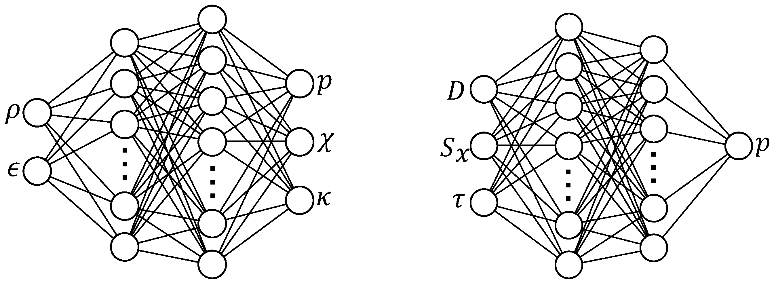
The NNEOS layouts for each type are summarized in

Table 1. Hyperparameters and errors for the NNs considered in this work. All NNs use two hidden layers (H.L.), both using a Sigmoid activation function, while all output layers use a ReLU activation function. The respective test datasets are used to evaluate the accuracy of the representations. Both error norms are shown.

Network	Size of H.L.		Error $\mathbf{\Delta }\mathit{p}$		Error $\mathbf{\Delta }\mathit{\chi }$		Error $\mathbf{\Delta }\mathit{\kappa }$
	H.L. 1	H.L. 2	${\mathit{L}}_1$	${\mathit{L}}_{\mathbf{\infty }}$	${\mathit{L}}_1$	${\mathit{L}}_{\mathbf{\infty }}$	${\mathit{L}}_1$	${\mathit{L}}_{\mathbf{\infty }}$
NNEOSA	600	300	$2.13·{10}^{-4}$	$6.16·{10}^{-3}$	$6.03·{10}^{-4}$	$1.81·{10}^{-1}$	$2.58·{10}^{-3}$	$1.15·{10}^{-1}$
NNEOSB	400	600	$1.03·{10}^{-4}$	$2.52·{10}^{-3}$	$4.97·{10}^{-5}$	$5.11·{10}^{-4}$	$7.66·{10}^{-5}$	$9.28·{10}^{-4}$
NNC2PS	600	200	$3.84·{10}^{-4}$	$8.14·{10}^{-3}$	-	-	-	-
NNC2PL	900	300	$3.62·{10}^{-4}$	$9.26·{10}^{-3}$	-	-	-	-

and NNEOSB is visualized on the left of Figure 1. For the training, an initial learning rate of the Adam optimizer [23] is set to $1·{10}^{-4}$ ($6·{10}^{-4}$) for the training of NNEOSA (NNEOSB) and automatically adapted when saturations of the error on the training dataset occurred. The training is completed when the training error does not continue to decrease even after learning rate adaptions (see Appendix B for an example of the training of NNEOSA). Comparing to the test dataset after training, the difference in the error of the returned pressure p is within the same order of magnitude for both networks, but it is approximately twice as large for NNEOSA in both the $L_1$ and $L_{\infty }$ norms. As expected, NNEOSB returns much more accurate values for the derivatives of the pressure as, unlike NNEOSA, it is specifically trained to return these as outputs. As measured in the $L_1$-norm ($L_{\infty }$-norm), we find that the error in the derivative $\chi$ in NNEOSB is a factor of ∼12 (354) smaller than that of NNEOSA and a factor of ∼34 (124) smaller for the derivative $\kappa$.

2.2. NN for C2P

As a second approach, NNs are built to represent the entire C2P transformation. These NNs output the pressure p from the three conserved quantities in $\mathbf{u}$. All the other primitive quantities are then computed analytically from the conserved variables and the pressure, see Appendix A.

The EOS parameter is again $\mathsf{\Gamma }=5/3$. The training dataset is constructed by uniformly sampling the primitive variables over the following intervals $\rho \in (0,10.1),ϵ\in (0,2.02),v_x\in (0,0.721)$, and then calculating the corresponding conservative variables through Equation (2). The training and test datasets contain $80,000$ and $10,000$ samples respectively, and random mini-batches of a size of 32 were used for the training process.

When choosing an NN architecture, a balance between accuracy and speed must be found. In order to investigate the differences in larger versus smaller NN, two NN representations of the C2P differing in the number of neurons are considered:

 NNC2PS 

Type S NN outputs the pressure from the conservative variable using a small number of neurons that still guarantee pressure errors of order ∼${10}^{-4}$, as for the NNEOS.

 NNC2PL 

Type L NN has a larger size but it is otherwise identical to NNC2PS.

The networks’ architecture is visualized on the right of Figure 1. The NNC2P layout for each type is summarized in Table 1. They are trained with a learning rate of $6·{10}^{-4}$ and learning rate adaptions until the error on the training dataset is minimized (an example of the training of NNC2PS can be found in Appendix B). Again we measure the error in the calculated pressure after the trained NN performs the C2P by comparing to a test dataset. Here we find that both NNC2PS and NNC2PL perform very similarly, with an NNC2PL returning an error smaller by a factor of 1.06 in the $L_1$ norm. We also note that this error is consistent in size with the errors in the pressure produced by NNEOSA and NNEOSB, being the same order of magnitude, with NNEOSB returning errors a factor ∼4 (3.5) smaller than NNC2PS (NNC2PL) in the $L_1$-norm. Since the NN performs the entire C2P, we do not need to perform the intermediate step of calculating the derivatives of the pressure in this case.

3. Results

In this section we present comparative timing and accuracy tests of the developed NNs. Section 3.1 directly considers different C2P algorithms using NNs and compares them against a standard algorithm for the C2P used in current numerical relativity simulations of neutron stars spacetimes [17,18,19]. Section 3.2 and Section 3.3 consider the use of different C2P algorithms with NNs in two standard 1D benchmarks for relativistic hydrodynamics implementations: a relativistic shock tube (problem 1 of [1]) and the evolution of a smooth density profile.

In order to properly evaluate the benefits of NN representation of the EOS and C2P in a realistic and yet controlled benchmark, the EOS in Equation (3) is stored as a table and evaluated via an eight point (3D) linear Lagrangian interpolation [26]. The tables contain a logarithmic grid of 500 values of the density $\rho$ and the temperature T (the specific internal energy is tabulated from $ϵ=1/(\mathsf{\Gamma }-1)N_A{k}_{B}T$, where $N_A$ is the Avogadro number and $k_B$ the Boltzmann constant) and a linear grid of 500 dummy values of the electron fraction $Y_e$. The grids are of the same range as the training dataset of the NNs, i.e., with maximum values 10% over the maxima of the shock tube test problem. The derivatives needed for the root-finders are taken from the linear interpolation.

The following tests are performed using either a standard C2P procedure based on Newton–Raphson (NR) algorithm and described in Appendix A (hereafter referred to as the NR algorithm) with the analytical, tabular, NNEOSA or NNEOSB representation of the EOS or the NNC2PS and the NNC2PL representation of the C2P procedure. A tolerance level of ${10}^{-8}$ is employed in the Newton–Raphson algorithm.

3.1. Accuracy and Timing of C2P

The accuracy of the NNs is evaluated on linear sampling $(\rho ,ϵ)$ on ranges $\rho \in [0.05,10]$ and $ϵ\in [0.01,2]$ with $n=200$, inverting the conservatives with varius C2P algorithms and comparing to the exact values. The considered C2P algorithms are:

• The NR algorithm with the analytical EOS;
• The NR algorithm with the EOS in tabulated form;
• The NR algorithm with the NNEOSA and NNEOSB representation of the EOS;
• The NNC2PS and NNC2PL algorithms.

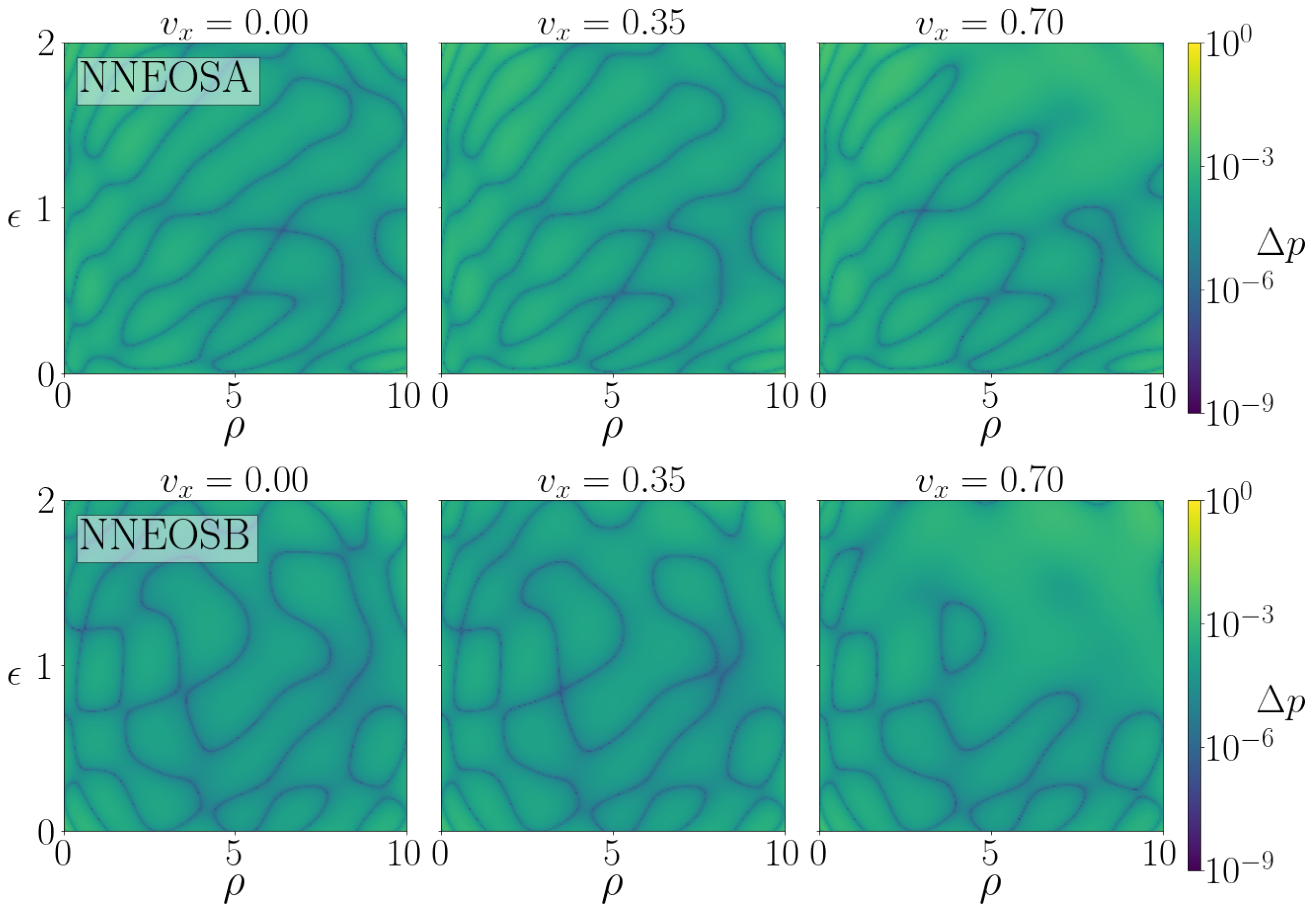
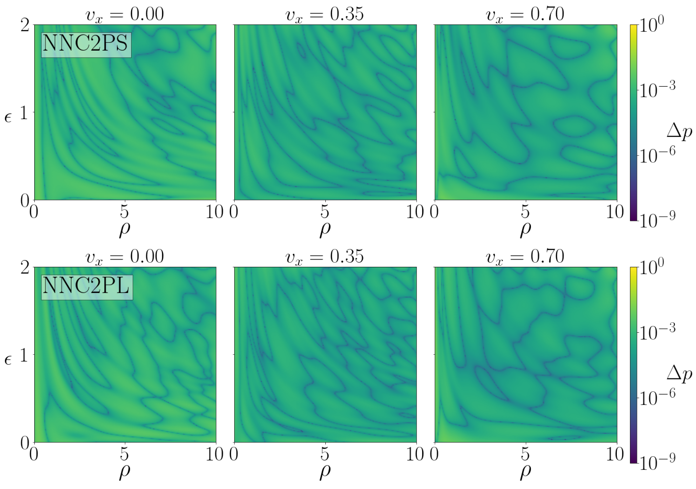
Figure 2 and Figure 3 report the absolute errors in the recovery of pressure as a function of $(\rho ,ϵ)$ in the testing datasets for the NR algorithm with the NN EOS representation and the NNC2P algorithms respectively.

The best attainable accuracy is given by the tolerance of the NR algorithm, ${10}^{-8}$, when taken with the analytical EOS. When combined with the tabulated EOS, we find that the errors grow to an average value of $1.4·{10}^{-3}$ for all three velocity values considered in Figure 2 and Figure 3. The maximum error reaches $1.04·{10}^{-2}$ for the highest velocity $v_x=0.7$, and it is dominated by the contribution from the table interpolation. The accuracy of the NNs proves superior to the tabulated EOS. Firstly we consider the NNs for evaluation of the EOS coupled with the NR algorithm. For the range of velocities shown NNEOSA has an average error ranging from $2.03·{10}^{-4}$ to $3.44·{10}^{-4}$, while NNEOSB ranges from $9.80·{10}^{-5}$ to $2.34·{10}^{-4}$. The latter is an order of magnitude smaller than the error with tabulated EOS. As expected, NNEOSB performs up to a factor of two better than NNEOSA. The maximum error of NNEOSA is comparable to the tabulated EOS; however, the maximum error of NNEOSB is almost an order of magnitude better ($2.29·{10}^{-3}$). Again, the size of the errors here demonstrate that the tolerance of the NR algorithm is much lower than the contribution to the error from the NN evaluation of the EOS. Secondly we consider the NNs which evaluate the total C2P, NNC2PS and NNC2PL. Here we find the range of average errors for NNC2PS $3.53·{10}^{-4}$–$9.73·{10}^{-4}$ and NNC2PL $2.99·{10}^{-4}$–$9.25·{10}^{-4}$ to be up to an order of magnitude superior to the tabulated EOS and at worst a factor of $\sim 1.4$ better. The maximum error for either NN is found for the highest velocity in NNC2PL of $9.66·{10}^{-3}$, ∼10% better than the tabulated EOS. As expected we find that NNC2PL has slightly smaller average errors than NNC2PS, reducing errors between a factor of 1.05 and 1.18 in the three representative velocities considered. Finally, we compare the two sets of NNs to each other. As it can be seen from the ranges quoted above, the average errors of all four NNs are of a consistent order of magnitude ∼${10}^{-4}$, with the lowest errors in the EOS, rather than C2P NNs, with NNEOSB performing between a factor of 1.8 and 9.9 better than the C2P NNs in terms of average error.

Timing tests are performed in a similar manner to accuracy tests but with building grids of states of increasing size from $n=100$ to $n=3200$. The results are summarized in

Table 2. Timing test of C2P with different algorithms and for different grid sizes n. The average time per call of different C2P schemes (analytic 2d EOS, interpolated 3d EOS, NN representation of the EOS, NN representations of the C2P are given). In addition, the speedup (acc.) with respect to the interpolated EOS is shown. Note that a C2P call transforms all grid points.

Grid Size	Analyt.	Interp.	NNEOSA		NNEOSB		NNC2PS		NNC2PL
	[${10}^{-4}$ s]	[${10}^{-2}$ s]	[${10}^{-3}$ s]	acc.	[${10}^{-3}$ s]	acc.	[${10}^{-3}$ s]	acc.	[${10}^{-3}$ s]	acc.
100	$2.45$	$1.56$	$4.94$	$3.15$	$2.69$	$5.79$	$0.98$	$15.83$	$1.23$	$12.71$
200	$2.79$	$2.70$	$6.76$	$3.99$	$3.65$	$7.38$	$1.12$	$24.13$	$1.90$	$14.17$
400	$3.33$	$4.91$	$12.28$	$4.00$	$6.49$	$7.58$	$1.82$	$27.02$	$3.71$	$13.23$
800	$4.58$	$9.39$	$22.40$	$4.19$	$13.95$	$6.73$	$4.16$	$22.57$	$6.84$	$13.73$
1600	$6.64$	$18.46$	$44.05$	$4.19$	$25.67$	$7.19$	$8.46$	$21.82$	$13.96$	$13.23$
3200	$10.99$	$36.10$	$83.86$	$4.30$	$49.06$	$7.36$	$16.25$	$22.21$	$26.82$	$13.46$

. As expected, all NN representations perform significantly slower than the NR algorithm with analytic EOS. Moreover, the cost of all the algorithms that do not employ the analytical EOS representation increases proportionally to the grid size. All the algorithms employing NN representations perform significantly faster than the NR algorithm with tabulated EOS. This is primarily due to the nested iteration of the NR scheme, see Appendix A. The NR algorithm using the NNEOSB runs up to two times faster than the same with NNEOSA, despite the fact that NNEOSB is a larger NN. This is due to the different computations of the derivatives of p: while NNEOSB returns the pressure and its derivatives as outputs, NNEOSA returns only the pressure, and then the pressure derivatives must be calculated from backpropagation. This latter procedure increases the run time of the evaluation. e.g., for $n=800$ gridpoints, generating an output with NNEOSB takes on average $6.07·{10}^{-3}$ s. While NNEOSA only needs $4.61·{10}^{-3}$ s to compute p, an additional $5.68·{10}^{-3}$ s are needed to compute the derivatives via backpropagation. Following expectations, the NNC2PL is slower (by on average a factor of more than 1.5) than the NNC2PS. While faster NN EOS representations are always achievable by limiting the network size, this can compromise accuracy. The most significant result is however the comparison of the NNC2P with the NR algorithm using the interpolated EOS. The NNC2PL completes the C2P on average ∼13 times faster than the NR algorithm with interpolated EOS. NNC2PS is instead ∼22 times faster. Thus, these NNs accelerate the C2P by more than an order of magnitude without significantly compromising the accuracy. We note also that, for all grid sizes, both NNC2P approaches are always faster than both NNEOS approaches, with the faster EOS approach (NNEOSB) slower than the slowest C2P approach (NNC2PL) by at least a factor of 1.7.

3.2. Shock Tube

We consider here the 1D shock tube problem discussed in [1] where the initial left/right states are given by $p=(13.33,{10}^{-6})$ and $\rho =(10,1)$ and the initial velocity is zero. The EOS is given by Equation (3) with $\mathsf{\Gamma }=5/3$. The exact solution of the Riemann problem exists and can be computed, e.g., with the method given in references [1,27,28]. Initial data are evolved with a standard HRSC algorithm using the HLLE flux [29], linear reconstruction of primitive variables with centered monotonized limiters and a third order Runge–Kutta time integration with Courant–Friedrich–Lewi factor of 0.5.

In the left panel of Figure 4 we demonstrate the numerical evolution of the shock tube problem using NNEOSA, NNEOSB and an analytical evaluation of the EOS to recover primitive variables. As a reference, the exact solution of the shock tube problem is also displayed. Here we observe a close agreement between all three approaches and the exact solution. Similarly, the right panel of Figure 4 compares the performance of NNC2PS and NNC2PL with the analytical evaluation of the equation of state, as well as a comparison with an interpolation of an EOS table. Again the NN approaches provide a close agreement with the exact solution.

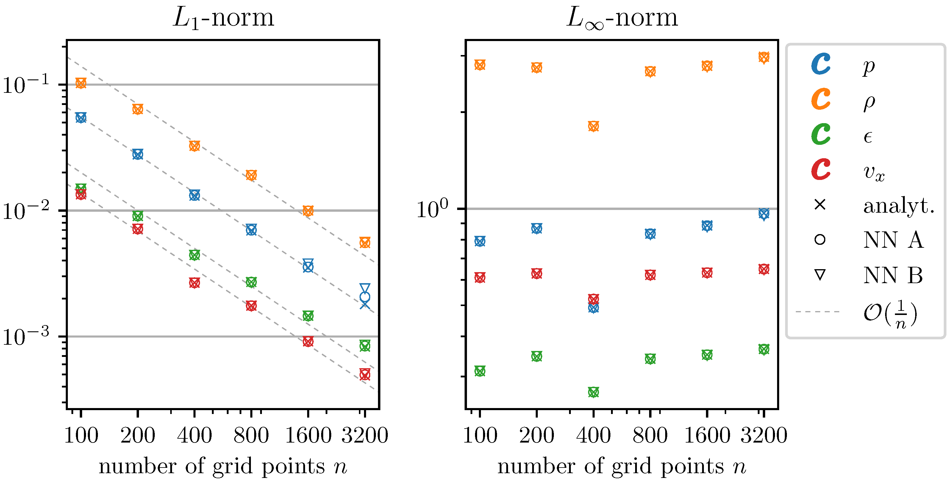
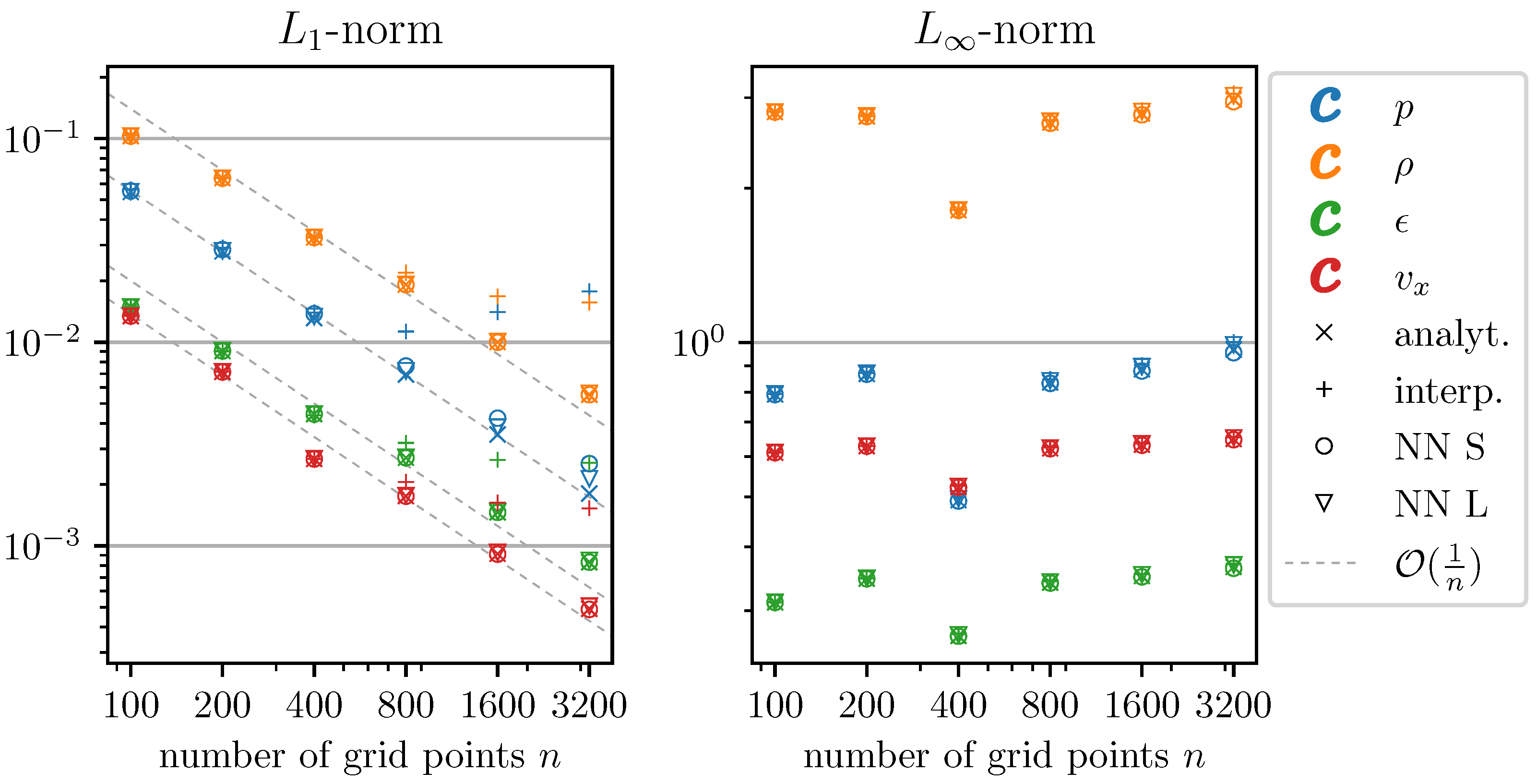
The respective errors between these methods are shown in Figure 5 and Figure 6. Firstly in Figure 5 (left) we demonstrate the $L_1$ norm of the error between the exact solution and the three EOS evaluation approaches used: analytical, NNEOSA and NNEOSB. Consistent with the numerical methods used, and the discontinuous nature of the shock tube profile, we find that the $L_1$ norm converges at first order, as demonstrated by dashed lines. When comparing the two NNs we find that the error in NNEOSA is consistent with that in NNEOSB and in fact for the largest grid sizes is slightly superior in the calculation of the pressure, by $\sim 17\%$, despite the superior performance detailed in Table 1. This results from the error in the NNs in representing the initial data of the shock tube problem, with NNEOSA representing the initial pressure in the right state with an error of $\sim 1·{10}^{-6}$, whereas NNEOSB returns a value deviating several orders of magnitude more (error of $\sim 5·{10}^{-4}$). As demonstrated in Figure 5, however, any loss of accuracy in replacing the analytic EOS evaluation with either NN is minimal.

In Figure 5 (right) we observe that, as in the $L_1$-norm, the errors in both NNs and the analytic EOS evaluation are consistent with each other. Here, however, we fail to see the error converging at the expected first order as the resolution increases. This is as a result of the $L_{\infty }$-norm selecting the point of our domain with maximum error, the location of the shock wave in the shock tube problem (shown at point $x\approx 0.83$ in Figure 4), at which specific point the HRSC algorithm fails to converge.

For the case in which the entire C2P is replaced by an NN, we show the $L_1$-norm of the errors in Figure 6 (left). Here we again show the expected first order convergence with dashed lines and include the case of the NR algorithm with the EOS in tabulated form. For lower resolutions (up to 800 grid points) we see first order convergence for all four methods. Beyond this resolution we see the interpolated tabulated EOS fails to converge in all variables due to the resolution of the EOS tables, while both NNC2PS and NNC2PL continue to converge at higher resolutions. For all primitives other than the pressure, we see almost identical performances between the remaining three approaches, whereas for the pressure, we see that, as expected, the analytical evaluation of the EOS is most accurate, followed by NNC2PL and then NNC2PS.

In Figure 6 (right) we demonstrate the error as calculated in the $L_{\infty }$-norm. As discussed above for the NNEOS approach, due to the failure of convergence of the HRSC algorithm at the shock wave, the error fails to converge in this norm. However, we again see a consistent error between all three schemes demonstrated, and, at the highest resolution, begin to see that NNC2PS slightly outperforms the other approaches when calculating the density and pressure. Finally, in Figure 7 we compare the errors of all four NN approaches. In Figure 7 (left), for the $L_1$-norm we observe that the errors in all methods are of a consistent order of magnitude. For the pressure, we see that at the highest resolution the best performance is found using NNEOSA, followed closely by NNC2PL, with the performance in all other variables and at all other resolutions being indistinguishable in terms of accuracy.

3.3. Smooth Sine-Wave

In addition to the shock tube problem, we also test this approach on a smooth sine wave profile. In contrast to the shock tube problem, the smooth nature of this test should allow us to investigate the higher order convergence properties which are absent in the presence of discontinuities formed in the shock tube problem. The initial profile of the fluid is given by

$$\begin{array}{cc}\hfill p=1,\rho & =1+0.2·sin(2\pi x),v_x=0.2,\hfill \end{array}$$

(9)

over the interval $x\in [-1,1]$ and periodic boundary conditions are imposed. The same EOS and HRSC algorithm as above is employed for the numerical solution.

In the left panel of Figure 8 we demonstrate the agreement between the exact sinewave data after evolving for a single period and the numerically evolved data after the same time calculated with an analytic evaluation of the equation of state, compared with NNEOSA and NNEOSB. Similarly, the right panel of Figure 8 demonstrates the agreement between the exact sinewave profile and the numerical data obtained through evolution using NNC2PS, NNC2PL, an analytical evaluation of the EOS and through interpolating a tabulated EOS.

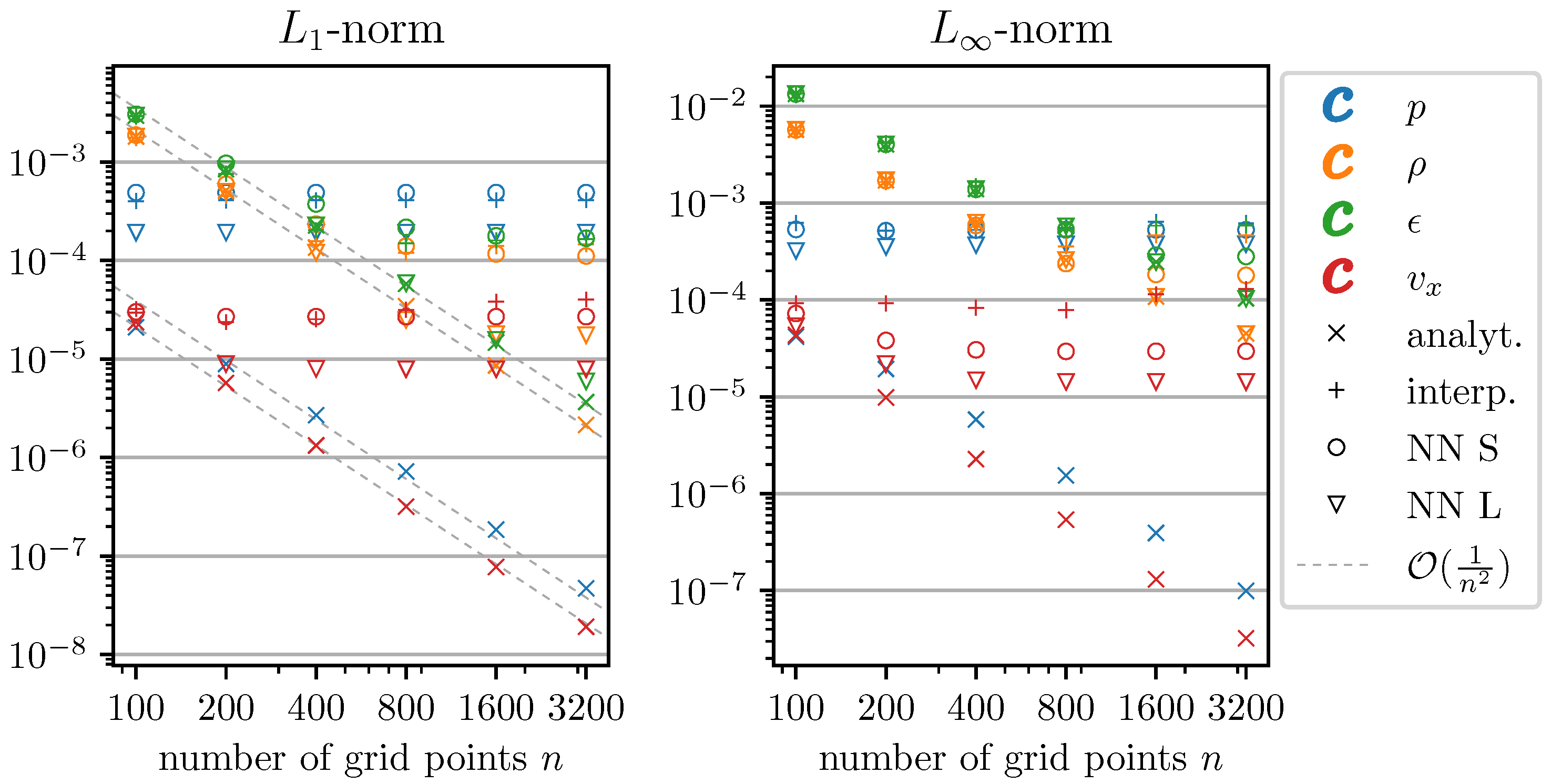
We again demonstrate the error properties of these evolved numerical data in further detail. Firstly the $L_1$-norm of the error for NNEOSA and NNEOSB is shown in Figure 9 (left). In contrast to the shock tube problem above, the smooth nature of the profile leads us to expect second order convergence, demonstrated by dashed lines. As expected, we see perfect second order convergence when the EOS is evaluated analytically; however, for both NNs we see the error saturate at a floor value (note the absolute values of these errors are considerably smaller than those for the shock tube above). This behavior arises as the error in the EOS representation is independent of the grid resolution, and so, for a small enough grid spacing, will eventually dominate the error arising from the HRSC scheme. The values at which the NN errors dominate, and therefore convergence is lost, are consistent with the accuracies in Table 1 of $\sim {10}^{-4}$ accuracy in pressure. In Figure 9 (right) we see similar behavior for the $L_{\infty }$-norm with slightly larger floor values consistent with the slightly larger values reported in Table 1 for the $L_{\infty }$-norm. Overall we see that NNEOSB consistently provides smaller errors than NNEOSA. We further note that this floor value in error could be reduced by enlarging the size of the NN, with the trade-off of making the EOS calculation slower and more expensive.

For NNC2PS and NNC2PL the $L_1$ norm of the error is shown in Figure 10 (left), again with second order convergence denoted by a dashed line. As before, we see that the analytic EOS call converges perfectly, with the NNC2PS and the interpolated tabulated EOS converging until a floor value in the error is reached. In contrast, however, NNC2PL performs better than the other NNs, and, while the error in certain quantities such as the pressure and velocity saturate almost immediately, the error in the internal energy $ϵ$ still converges and does not appear to have reached its minimum value at the highest resolution used, $n=3200$. In the $L_1$-norm we find that NNC2PL outperforms NNC2PS in all primitive variables, and, for $n\ge 400$ NNC2PL outperforms the tabulated EOS also. At the highest resolution we find that NNC2PL outperforms NNC2PS by a factor of $\sim 2.6$ and the tabulated EOS by a factor of $\sim 2$ for the error in the pressure and, for the internal energy, which is still converging, this factor increases to $\sim 29$ compared to NNC2PS and $\sim 28$ compared to the tabulated EOS.

In Figure 9 we see that even on the coarsest grid used, $n=100$, the error in the NNEOSA representation of the velocity is about a factor three larger than the analytic EOS representation. In contrast, when replacing the entire C2P with an NN, we see in Figure 10 that at this resolution the velocity error is now comparable to the analytic value. In Figure 11 (left) we compare the error between all NN approaches in the $L_1$-norm. Here we can see that, once the error has saturated at its floor value for the velocity and density, NNC2PL provides the lowest errors, performing an order of magnitude better than NNEOSA. This is also true for the specific internal energy which has not saturated its error at the highest resolution measured. In contrast, once the error has saturated, NNEOSB gives the lowest error for the pressure, performing an order of magnitude better than NNC2PS and a factor $\sim 4.5$ better than NNC2PL.

As above we see a similar picture in the $L_{\infty }$-norm albeit with larger absolute errors.

4. Conclusions

In this work, we explored artificial neural networks (NN) for the transformation of conservative quantities to primitives (C2P) in relativistic hydrodynamics. Working in a controlled yet complete framework, we demonstrated that the EOS evaluation or, alternatively, the entire C2P variables transformation can be substituted by simple and efficient NNs.

Our tests show that an NN representation of the EOS, either outputting the pressure (NNEOSA) or also including pressure derivatives (NNEOSB), can speed up by a factor between 3.1 and 7.4 standard C2P algorithms based on root-finders that are called 3D tabulated EOS. Moreover, the C2P employing NNEOSB runs up to two times faster than the same with NNEOSA, despite being a larger NN. This is due to the cost of the backpropagation needed to compute derivatives for NNEOSA and highlights an advantage of an NN including derivatives as regular output. The average error reached in the pressure recovery is of order of magnitude ${10}^{-4}$ for NNEOSA and NNEOSB, an order of magnitude smaller than that obtained with a tabulated EOS of typical size, with NNEOSB also outperforming NNEOSA and the tabulated EOS by an order of magnitude in its maximum error. These accuracies allow the use of the NNs in full hydrodynamical evolutions. Standard 1D benchmarks in special relativity indicate that the error of the NN EOS representation does not significantly affect solutions of Riemann problems up to very high resolutions of $n=3200$ grid points. This result is expected to hold also in multi-dimensional simulations since in those cases shocks and other elementary waves are resolved with fewer grid points. Note that at such high resolutions table interpolation errors can instead affect the convergence of the solution, as demonstrated by our tests. Similar considerations hold for smooth solutions. The second order convergence of a smooth flow solution is lost as the errors reach the finite precision of the NN representing the EOS. However, this issue is expected to arise also when using EOS tables and interpolation. We further note that, since any given physical EOS model (based for example on tabulated data) will only be accurate up to a certain error, an NN based on such a model should only be trained to a matching level of precision.

Our results indicate that an NN representation of the entire C2P is overall more effective than an NN representation of the EOS solely. In this case, the acceleration of the C2P algorithm is significant when compared to root-finding algorithms with multi-dimensional (3D) table interpolation for the EOS. In the discussed benchmarks, the speedup for the C2P is about a factor $\sim 13$ for the larger NN (NNC2PL) up to $\sim 22$ for the smaller NN (NNC2PS), thus depending mainly on the NN size. Our NNs aim to balance speed and accuracy, though further experimentation may be able to further improve this performance. NNC2PL significantly exceeded the accuracy of the solutions with EOS table interpolation in both shock-tube and sinewave benchmarks, with all primitives calculated more accurately up to an improvement by a factor of ∼28 still allowing a speed-up of more than an order of magnitude. The benchmark tests also show that, for a shock-tube problem with larger overall errors, the two approaches of NNEOS and NNC2P give similar errors, with NNEOSA improving the accuracy of NNC2PL by $\sim 4\%$. However, for a sinewave problem with smaller overall errors, NNC2PL gives the most accurate calculation of the velocity, density and internal energy, outperforming NNEOSB by up to a factor of ∼9.2, while NNEOSB performs best on the pressure outperforming NNC2PL by a factor of ∼4.5. We also remark that the time needed for a C2P using a standard root finder also depends on the problem it is applied on: large and sudden changes, e.g., of shock waves and other discontinuities, cause more iterations of the root-finding algorithms and thus need more time. An NN representation of the C2P does not suffer from this drawback and thus can also improve the robustness of the simulation.

In summary, the results reported in this paper indicate clear advantages in including machine learning representations of the C2P in relativistic hydrodynamics. Going beyond these preliminary tests, future work will investigate the applicability of our findings to full multi-dimensional simulations in relativistic astrophysics.

References

1. Martí, J.M.; Müller, E. Numerical Hydrodynamics in Special Relativity. Living Rev. Relativ. 2003, 6, 7. [Google Scholar] [CrossRef] [PubMed] [Green Version]
2. Timmes, F.X.; Swesty, F.D. The Accuracy, Consistency, and Speed of an Electron-Positron Equation of State Based on Table Interpolation of the Helmholtz Free Energy. Astrophys. J. Suppl. 2000, 126, 501–516. [Google Scholar] [CrossRef]
3. Lattimer, J.M.; Swesty, F.D. A Generalized equation of state for hot, dense matter. Nucl. Phys. 1991, A535, 331–376. [Google Scholar] [CrossRef]
4. Anile, A.M. Relativistic Fluids and Magneto-Fluids: With Applications in Astrophysics and Plasma Physics; Cambridge Monographs on Mathematical Physics; Cambridge University Press: Cambridge, UK, 1989. [Google Scholar] [CrossRef]
5. Toro, E.F. Riemann Solvers and Numerical Methods for Fluid Dynamics, 2nd ed.; Springer: Berlin/Heidelberg, Germany, 1999. [Google Scholar]
6. LeVeque, R.J. Finite Volume Methods for Hyperbolic Problems; Cambridge University Press: Cambridge, UK, 2002. [Google Scholar]
7. Blandford, R.; Meier, D.; Readhead, A. Relativistic Jets from Active Galactic Nuclei. Ann. Rev. Astron. Astrophys. 2019, 57, 467–509. [Google Scholar] [CrossRef] [Green Version]
8. Janka, H.T. Explosion Mechanisms of Core-Collapse Supernovae. Ann. Rev. Nucl. Part. Sci. 2012, 62, 407–451. [Google Scholar] [CrossRef] [Green Version]
9. Font, J.A. Numerical hydrodynamics and magnetohydrodynamics in general relativity. Living Rev. Rel. 2007, 11, 7. [Google Scholar] [CrossRef] [Green Version]
10. Radice, D.; Bernuzzi, S.; Perego, A. The Dynamics of Binary Neutron Star Mergers and GW170817. Ann. Rev. Nucl. Part. Sci. 2020, 70, 95–119. [Google Scholar] [CrossRef]
11. Bernuzzi, S. Neutron Star Merger Remnants. Gen. Rel. Grav. 2020, 52, 108. [Google Scholar] [CrossRef]
12. Noble, S.C.; Gammie, C.F.; McKinney, J.C.; Del Zanna, L. Primitive Variable Solvers for Conservative General Relativistic Magnetohydrodynamics. Astrophys. J. 2006, 641, 626–637. [Google Scholar] [CrossRef] [Green Version]
13. Siegel, D.M.; Mösta, P.; Desai, D.; Wu, S. Recovery schemes for primitive variables in general-relativistic magnetohydrodynamics. Astrophys. J. 2018, 859, 71. [Google Scholar] [CrossRef]
14. Kastaun, W.; Kalinani, J.V.; Ciolfi, R. Robust Recovery of Primitive Variables in Relativistic Ideal Magnetohydrodynamics. Phys. Rev. D 2021, 103, 023018. [Google Scholar] [CrossRef]
15. Sekiguchi, Y.; Kiuchi, K.; Kyutoku, K.; Shibata, M. Dynamical mass ejection from binary neutron star mergers: Radiation-hydrodynamics study in general relativity. Phys.Rev. 2015, D91, 064059. [Google Scholar] [CrossRef] [Green Version]
16. Foucart, F.; O’Connor, E.; Roberts, L.; Kidder, L.E.; Pfeiffer, H.P.; Scheel, M.A. Impact of an improved neutrino energy estimate on outflows in neutron star merger simulations. Phys. Rev. 2016, D94, 123016. [Google Scholar] [CrossRef] [Green Version]
17. Radice, D.; Perego, A.; Hotokezaka, K.; Fromm, S.A.; Bernuzzi, S.; Roberts, L.F. Binary Neutron Star Mergers: Mass Ejection, Electromagnetic Counterparts and Nucleosynthesis. Astrophys. J. 2018, 869, 130. [Google Scholar] [CrossRef] [Green Version]
18. Bernuzzi, S.; Breschi, M.; Daszuta, B.; Endrizzi, A.; Logoteta, D.; Nedora, V.; Perego, A.; Radice, D.; Schianchi, F.; Zappa, F.; et al. Accretion-induced prompt black hole formation in asymmetric neutron star mergers, dynamical ejecta and kilonova signals. Mon. Not. Roy. Astron. Soc. 2020, 497, 1488–1507. [Google Scholar] [CrossRef]
19. Nedora, V.; Bernuzzi, S.; Radice, D.; Daszuta, B.; Endrizzi, A.; Perego, A.; Prakash, A.; Safarzadeh, M.; Schianchi, F.; Logoteta, D. Numerical Relativity Simulations of the Neutron Star Merger GW170817: Long-Term Remnant Evolutions, Winds, Remnant Disks, and Nucleosynthesis. Astrophys. J. 2021, 906, 98. [Google Scholar] [CrossRef]
20. Goodfellow, I.; Bengio, Y.; Courville, A. Deep Learning; MIT Press: Cambridge, MA, USA; London, UK, 2016. [Google Scholar]
21. Mehta, P.; Bukov, M.; Wang, C.H.; Day, A.G.R.; Richardson, C.; Fisher, C.K.; Schwab, D.J. A high-bias, low-variance introduction to Machine Learning for physicists. Phys. Rep. 2019, 810, 1–124. [Google Scholar] [CrossRef] [PubMed]
22. Schmidhuber, J. Deep Learning in Neural Networks: An Overview. Neural Netw. 2015, 61, 85–117. [Google Scholar] [CrossRef] [Green Version]
23. Kingma, D.P.; Ba, J. Adam: A Method for Stochastic Optimization. arXiv 2014, arXiv:1412.6980. [Google Scholar]
24. Paszke, A.; Gross, S.; Massa, F.; Lerer, A.; Bradbury, J.; Chanan, G.; Killeen, T.; Lin, Z.; Gimelshein, N.; Antiga, L.; et al. PyTorch: An Imperative Style, High-Performance Deep Learning Library. In Advances in Neural Information Processing Systems 32; Wallach, H., Larochelle, H., Beygelzimer, A., d’Alché-Buc, F., Fox, E., Garnett, R., Eds.; Curran Associates, Inc.: New York, NY, USA, 2019; pp. 8024–8035. [Google Scholar]
25. Harris, C.R.; Millman, K.J.; van der Walt, S.J.; Gommers, R.; Virtanen, P.; Cournapeau, D.; Wieser, E.; Taylor, J.; Berg, S.; Smith, N.J.; et al. Array programming with NumPy. Nature 2020, 585, 357–362. [Google Scholar] [CrossRef]
26. O’Connor, E.; Ott, C.D. A new open-source code for spherically symmetric stellar collapse to neutron stars and black holes. Class. Quantum Gravity 2010, 27, 114103. [Google Scholar] [CrossRef] [Green Version]
27. Martí, J.M.; Müller, E. The analytical solution of the Riemann problem in relativistic hydrodynamics. J. Fluid Mech. 1994, 258, 317–333. [Google Scholar] [CrossRef]
28. Mach, P. Analytic solutions of the Riemann problem in relativistic hydrodynamics and their numerical applications. Acta Phys. Pol. Proc. Suppl. 2009, 2, 575. [Google Scholar]
29. Harten, A.; Lax, P.D.; van Leer, B. On Upstream Differencing and Godunov-Type Schemes for Hyperbolic Conservation Laws. SIAM Rev. 1983, 25, 35–61. [Google Scholar] [CrossRef]
30. Wilson, J.R.; Mathews, G.J. Relativistic Numerical Hydrodynamics; Cambridge University Press: Cambridge, UK, 2010. [Google Scholar] [CrossRef] [Green Version]
Figure 1. Schematic diagram of NNEOSB (left) and NNC2P (right). Input layers are on the left of each network and output layers are on the right. NNEOSA is identical to the scheme of NNEOSB but without the output neurons for χ and κ .
Symmetry 13 02157 g001
Figure 2. Accuracy of the NNEOS. Discrete per point evaluation of the accuracy of the NN EOS representations on a linear grid of ρ and ϵ values for three values of the velocity v x . The colors show the absolute deviation from the exact values (Equation (3)). Top (bottom) panels refer to NNEOSA (NNEOSB).
Symmetry 13 02157 g002
Figure 3. Accuracy of the NNC2P. Discrete per point evaluation of the accuracy of the NN C2P representations on a linear grid of ρ and ϵ values for three values of the velocity v x . The colors show the absolute deviation from the exact values (Equation (3)). Top (bottom) panels refer to NNC2PS (NNC2PL).
Symmetry 13 02157 g003
Figure 4. Solution to the shock tube problem at t = 0.4 as computed by different algorithms. Primitive variables are indicated with different colors; the exact solution is indicated in solid gray lines. The y axis represents the value of the primitive variables, rescaled by factors shown in the legend for readability. The left panel compares NNEOSA and NNEOSB to the exact solution and the solution obtained with the analytical EOS representation. The right panel compares NNC2PS and NNC2PL to the exact solution, the solution obtained with the NR algorithm and the analytical EOS representation and the tabular EOS. The numerical solutions are computed at a resolution of n = 100 grid points with step size of d t = 5 · 10 3 . The close agreement between the results using NNs and the results obtained with traditional C2P evaluations shows that the dominant source of error arises form the HRSC scheme used to solve the Euler equations and not the introduction of NNs.
Symmetry 13 02157 g004
Figure 5. Errors of NNEOS algorithms in the shock tube problem. L 1 (left) and L (right) norms of the solutions at t = 0.4 are shown for different primitive quantities. First order convergence in L 1 norm is measured in all quantities and for all algorithms.
Symmetry 13 02157 g005
Figure 6. Errors of NNC2P algorithms in the shock tube problem. L 1 (left) and L (right) norms of the solutions are shown for different primitive quantities. The slope of a first order convergence is illustrated by the dashed gray lines in the L 1 plot. First order convergence in L 1 norm is measured in all quantities and for all algorithms, up to the precision of the tabulated EOS.
Symmetry 13 02157 g006
Figure 7. Errors of NNC2P and NNEOS algorithms in the shock tube problem. L 1 (left) and L (right) norms of the solutions are shown for different primitive quantities. The slope of a first order convergence is illustrated by the dashed gray lines in the L 1 plot. First order convergence in L 1 norm is measured in all quantities and for all algorithms.
Symmetry 13 02157 g007
Figure 8. Solution to the sine-wave density profile at t = 5 (i.e., after one period) as computed by different algorithms Primitive variables are indicated with different colors; the exact solution is indicated in solid gray lines. The left panel compares NNEOSA and NNEOSB to the exact solution and the solution obtained with the analytical EOS representation. The right panel compares NNC2PS and NNC2PL to the exact solution, the solution obtained with the NR algorithm and the analytical EOS representation and the tabular EOS. The numerical solutions are computed at a resolution of n = 100 grid points with step size of d t = 10 2 .
Symmetry 13 02157 g008
Figure 9. Errors of NNEOS algorithms in the sine-wave density profile problem. L 1 (left) and L (right) norms at t = 5 of the solutions are shown for different primitive quantities. Second order convergence in L 1 norm is measured in all quantities and for all algorithms until the NN error dominates.
Symmetry 13 02157 g009
Figure 10. Errors of NNC2P algorithms in the sine-wave density profile problem. L 1 (left) and L (right) norms at t = 5 of the solutions are shown for different primitive quantities. Second order convergence in L 1 norm is measured in all quantities and for all algorithms until the NN error or precision of the tabulated EOS dominates.
Symmetry 13 02157 g010
Figure 11. Errors of NNC2P and NNEOS algorithms in the sine-wave density profile problem. L 1 (left) and L (right) norms at t = 5 of the solutions are shown for different primitive quantities.
Symmetry 13 02157 g011