
Dynamical Reason for a Cyclic Universe

School of Mathematical Science, Fudan University, Shanghai 200433, China
Symmetry 2021, 13(12), 2272; https://doi.org/10.3390/sym13122272
Submission received: 26 October 2021
/
Revised: 14 November 2021
/
Accepted: 19 November 2021
/
Published: 29 November 2021
(This article belongs to the Special Issue Physics and Mathematics of the Dark Universe)
Abstract
By analyzing the energy-momentum tensor and equations of state of ideal gas, scalar, spinor and vector potential in detail, we find that the total mass density of all matter is always positive, and the initial total pressure is negative. Under these conditions, by qualitatively analyzing the global behavior of the dynamical equation of cosmological model, we get the following results: (i) , namely, the global spatial structure of the universe should be a three-dimensional sphere ; (ii) , the cosmological constant should be zero or an infinitesimal; (iii) , the initial singularity of the universe is unreachable, and the evolution of the universe should be cyclic in time. Since the matter components considered are quite complete and the proof is very elementary and strict, these conclusions are quite reliable in logic and compatible with all observational data. Obviously, these conclusions will be very helpful to correct some popular misconceptions and bring great convenience to further research other problems in cosmology such as the properties of dark matter and dark energy. In addition, the macroscopic Lagrangian of fluid model is derived.
1. Introduction
In cosmology, we have two important constants to be determined. They are cosmic curvature K and cosmological constant . Some characteristic parameters of the universe, such as the age , Hubble constant , total mass density , etc., have been measured to high accuracy [1,2,3,4,5,6]. To determine the cosmic curvature K, the usual approach is to transform the Friedmann equation into an algebraic equation . In theory, can be judged by contrasting observational data or . From the observations we have , which is very close to the case of flat space. Considering measurement errors, it is hard to determine what type the space is. In fact, no matter what the case of spatial curvature is, for a young universe, it is easy to calculate that we always have . So this criterion is rather ambiguous.
Cosmological constant has a dramatic history. Since Einstein introduced in 1917 to get a static and closed universe, the debate over whether is zero or not has been repeated many times [7,8,9]. Now dark matter and dark energy are attracting the attention of scientists around the world, becoming the hottest topic, challenging traditional standard models of particle and cosmology. The usual description of dark matter and dark energy uses the equation of state and or , and many specific models have been obtained by fitting the observed data [7,8,9,10,11,12,13,14]. However, the problem is far from being solved [15].
In [12], by introducing the potential function , the Friedmann equations with some known dark energy models are converted into Hamiltonian dynamics, and the evolving trajectory is analyzed to explain the accelerating expansion of the universe. The literatures [16,17,18,19,20,21,22] provide some similar discussion on specific gravitational sources. The nonlinear scalar fields were discussed in reference [16,17,18] to obtain the cyclic universe model. In [19], a set of precise cyclic solutions with ordinary dust and radiation are obtained, and in [20], the exact solutions of ghost and electromagnetic fields are derived. The quantized nonlinear spinor fields and trajectories are calculated and a cyclic solution is solved in [21,22]. In [23,24], the authors use phase plane to discuss the dynamical behavior of the universe, and conclude that a cyclical universe is reasonable from a dynamical systems perspective, and requires in addition to standard cosmological assumptions, only two conditions: (i) the spatial sections must have positive spatial curvature , and (ii) the late time effective cosmological “constant” must decay fast enough as a function of the scale factor. Both of these conditions are consistent with all current observations to date. In 2008, M. Novello and S. E. Perez Bergliaffa reviewed the general features of nonsingular universes and cyclic universes, discussed the mechanisms behind the bounce, and analyzed examples of solutions that implement these mechanisms [25].
In [26], after analyzing the Planck Legacy 2018 release, the authors found enhanced gravitational lens amplitude in the power spectrum of the cosmic microwave background (CMB), which is different from the data of the standard CDM model. The cosmic space is more like a giant balloon that is closed and curved. The main task of the Planck satellite is to detect the tiny fluctuation of the CMB temperature. The study of the fluctuation of the CMB temperature is the key to uncover the relevant cosmological models and parameters. This information defines the expansion, composition and origin of the cosmic large-scale structure. The authors use ‘closed universe’ to explain this anomalous effect. The spectra are now more inclined to a positive curvature greater than 99% confidence level. The positive curvature can explain the anomalous amplitude of the gravitational lens.
This paper is a development of [21,27]. In [21], the calculations showed the term is a higher order infinitesimal as , so its influence on the behavior of the early universe is negligible. Some nonlinear effects of the matter fields should be important for the early behavior. The calculations show that the nonlinear potential of spinors leads to a higher order term , which is equivalent to negative pressure and becomes dominant factor for the behavior of the early universe. In [27], we showed that the global behavior of Friedmann equation is mainly determined by two hypotheses of positive mass density and initial negative pressure. In order to verify the reasonability of the two hypotheses, some contents were added continually, and we obtain the present paper.
Under two ordinary hypotheses for functions of state, namely the total mass density of all matter is always positive, and the initial total pressure is negative, by qualitatively analyzing the global behavior of the dynamical equation of cosmological model, we get the following results: the global spatial structure of the universe should be a closed 3-d sphere , the cosmological constant should be zero or a tiny number and the initial singularity of the universe is unreachable, and the evolution of universe should be cyclic in time. Obviously, these conclusions will be very helpful to correct some popular misconceptions and bring great convenience in further researching other problems in cosmology such as the properties of dark matter and dark energy.
2. Energy-Momentum Tensor of Matter
In order to understand the mystery and dynamically behavior of the universe, Energy-momentum tensor(EMT) and equation of state(EOS) of all kinds of matter are crucial factors. In this paper, we establish EMT and EOS of some elementary components according to credible theories in detail. Cosmology contains a variety of contents, so it is necessary to clarify the conventions and notations frequently used in the paper at first. The line element of the space-time is given by [28]
where and are tetrad expressed by Dirac matrices
which satisfies the Clifford algebra
The Pauli matrices are expressed by
where . We take as unit of speed. For index, we use the Greek characters for curvilinear coordinates, Latin characters for local Minkowski coordinates and for spatial indices. The Einstein’s summation is used.
Similarly to the case of metric , the definition of Ricci tensor can also differ by a negative sign. We take the definition as follows
Since the Lagrangian of a compound physical system is a superposable real scalar, in cosmology the Lagrangian of main kinds of gravitational sources is generally given by
in which , is the cosmological constant, the total Lagrangian of all matter.
where is the global slow-roll scalar field. is the Lagrangian of ideal dust, whose statistical average is perfect fluid model. is the speed of n-th particle in usual sense. is the Lagrangian for spinors with nonlinear potential , electromagnetic potential and strong short distance interaction , in which the momentum operator
where is current operator and spin operator. They are defined respectively by
is Keller connection and is Gu-Nester potential. They are calculated by [28,29,30,31].
If the metric of the space-time can be orthogonalized, we have , so the spin-gravity coupling term in cosmology. means taking real part of a complex number. In this paper we take the following simplest nonlinear potential as example to show its dynamical effects in cosmology
The Hamiltonian formalism and classical mechanics can be clearly described only in the Gu’s natural coordinate system [32]
where defines the Newton’s realistic cosmic time, which is different from the proper time of a particle . The Dirac- is defined as
which means . Only scalar, spinor and vector fields can construct a proper Lagrangian [22], so (7)–(10) become the representation of all kinds of matter. In cosmology, to study them clearly is enough for theoretical analysis.
Variation of the Lagrangian (6) with respect to , we get Einstein’s field equation
where is the Euler derivative, and is EMT of all matter defined by
In (21) for decomposition of metric.
So, we get the classical approximation for EMT of dark spinor with self-interaction
acts like negative pressure and takes the place of cosmological constant in Equation (16). If , the spinor moves along geodesic like a mass-point. Some researchers studied varying cosmological ‘constant’ [34,35,36,37,38,39,40,41], but a directly varying violates covariance of dynamics. The following calculation discloses that the main physical origin of a covariant may be just the nonlinear potential .
For energy-momentum tensor, we have the following useful theorem, which means the energy-momentum of any independent system is conserved respectively.
Theorem 1.
Assume matter consists of two subsystems I and II, namely , then we have
If the subsystems I and II have not interaction with each other, namely,
then the two subsystems have independent energy-momentum conservation laws respectively,
Proof.
By the definition of EMT (17), the variation is a linear mapping, so (27) holds. By (28), the variables and have decoupling dynamic equations. Since the dynamics of variables is sufficient condition of energy-momentum conservation law, we can derive from dynamic equation of , and from dynamic equation of independently, so (29) holds. The proof is completed. □
By Theorem 1, we find in (7) the slow-roll scalar have not interaction with other components of matter, so we have . In (8), each particle of ideal gas has not interaction with other components, so each particle satisfies energy-momentum conservation law. For k-th particle, by (20) we have
By , we get geodesic equation for k-th particle
Therefore, for ideal mass point, energy momentum conservation law is equivalent to dynamics. For perfect fluid model, also gives dynamical equations, but an additional equation of state is needed and some information of the system is lost in the simplification of fluid.
If or , spinor interacts with or , so we should take it as one system. For an isolated particle, the classical approximation of static or of the particle can be treated as an additional mass due to linearity of and . We calculate in the next section. The propagating is photon, which can be treated as massless particles. Thus except the global scalar , the classical approximation of EMT for other fields is usually depicted by
The statistical expectation of nonlinear potentials is function of state which acts like negative pressure. By (14) we find is scale dependent, so we have .
The following calculation discloses that the function of state may be partly the physical origin of cosmological ‘constant’ . By the energy-momentum conservation law of (32), we have equation of motion for dark spinor gas
3. Equation of State in Cosmology
3.1. Basic Relations and Assumptions for EMT
In cosmology, we have Friedmann-Lemaitre-Robertson-Walker(FLRW) metric
in which correspond to respectively. By symmetry we get
For all gravitational sources we have EMT in traditional form
The dynamics of cosmology (16) and are overdetermined due to high symmetry of FLRW metric. It is easy to check, among all dynamical equations, only the following equations are independent equations, but the spatial components of the Einstein’s field equations can be derived from these equations. So we have dynamics for FLRW universe as
where index i means independent subsystem. All other equations can be derived from the above equations. Together with initial values and equations of state , the above equations are closed and the solution is uniquely determined.
The analysis in the next section shows that the asymptotic property of P as is crucial for the fate of the universe, so we give detailed discussion on this problem. By (39) we have energy conservation law for all matter
If as , then we have
Since as , by (42) we certainly have as . Therefore, the existence of inflation in the early universe implies the initial negative pressure [11,12,13,14].
According to the above analysis, we have the following conclusions for total EMT (37) in general:
The total mass-energy density is always positive, namely
The total pressure when the universe is small enough, namely
These two conditions are the fundamental hypotheses of the following dynamical analysis, which are decisive for the evolution of the universe. Next, we give more discussions for the reasonability of the assumptions according to EOS of various materials.
3.2. Equation of State of Ideal gases
At first, we examine the ideal gases. To solve the geodesic of the particles, we prove a useful theorem.
Theorem 2.
Assume the line element of a manifold has the following form
then we have the first integral for the geodesic in the manifold,
where are integral constants.
Proof.
The nonzero Christoffel symbols are , and
where , . Since can be directly derived from (45), it is unnecessary to calculate and . Denoting , the geodesic equation of is given by
Multiplying on both sides we get
In the FLRW space-time (34), if a particle moves along r coordinate, then the first integral of its geodesic in this subspace-time can be solved as
where C is a constant determined by initial data. By (52) we get the drifting speed of n-th particle in usual sense
So the momentum of the particle satisfies
where is the proper mass of the particle. By the symmetry of the space-time, (54) holds for all particles. For the massless photons, it is easy to check that the wavelength , so their momentum p also satisfy (54); that is to say, (54) is also suitable for photon gas.
Now we establish the relation between the state functions of the ideal gases and scale factor a. By (54) we have , where are constants determined by initial data at . Then on the one hand, for all particles we have the average square momentum as
where is a constant only determined by initial data at .
On the other hand, the relativistic relation between momentum p and the kinetic energy is given by
so can be also calculated by statistics. Assuming the distribution of kinetic energy of the ideal gases is given by . Then it satisfies the equation of moments
where the second formula is the definition of temperature T of the gases, J/K is the Boltzmann constant, is a constant reflecting the distribution function of particles. In the case of Maxwell distribution [31], we have .
By (56) and the moments (57) we have
where is average proper mass of all particles. Comparing (58) with (55), we get the relation ,
where is a constant determined by initial data. We take a as independent variable in statistical calculation.
In microscopic view, the energy momentum tensor of ideal gas is given by (20). The average energy-momentum tensor takes the form (37). By (20), in average sense we have [31]
By (20) and (59) we have
where , and is the angular density of proper mass, which is a constant. Substituting (61) into energy conservation law (39) we get
While we find . Ideal gases cannot provide negative pressure.
In the above derivation, the FLRW metric (34) is used as piston-cylinder system to drive the ideal gas, and we can prove that the elastic collisions of particles have no influence on these results [31]. So the results are actually valid in general cases. By (59) we have relation
where J is dimensionless temperature. The above results conclude the following theorem.
Theorem 3.
For relativistic ideal gas, we have the EOS as
For adiabatic process the functions of state satisfy parameter equation
where J acts as independent variable, is a constant of density dimension.
The above derivation is compatible with relativity and includes the driving effect of gravity. In the case of low temperature, Theorem 3 gives the EOS for the adiabatic monatomic gas
which is identical to the empirical law of thermodynamics. Letting or , we get and the Stefan-Boltzmann’s law . Thus the above results are automatically suitable for photons, and the Stefan-Boltzmann’s law is also valid for the ultra-relativistic particles. In general relativity, all processes occur automatically, and is independent of any practical process. An EOS omitting the driving effect of gravity is invalid in general relativity.
3.3. Asymptotic Behavior of Scalar Field in the Early Universe
For scalar field , by (19) we have
In the case , we have , so we only need to consider the highest order term in . For potential , by variation with respect to we get dynamical equation
(68) can be also derived by substituting (67) into energy conservation law (39). If the universe has an initial singularity, we set . For low temperature particles, we have . By Friedmann Equation (38), we find while . So we assume in general
About the range of j, Barrow made some analysis in [43]. In the mode of accelerating expansion , we should have . Substituting (69) into (68) we get solution in the case of ,
Substituting into (71), we get
By (72), we find the nonlinear scalar provides initial negative pressure if . We have if , if and if .
In the case of , (68) is a linear equation of , and its solution is an oscillating function of . For asymptotic solution of (68) as , is a higher order infinity than , so we certainly have and then . The linear scalar cannot provides initial negative pressure. However, all asymptotic solutions are similar to the following one with ,
where are constants. The corresponding pressure is given by
which is also an oscillating function with . Of course, P becomes negative when is large enough. Substituting the above results into (67) we get
3.4. Equation of State of Spinor Gas
The above calculation shows that perfect fluid and scalar model cannot provide negative pressure. Now we examine the dark spinor with nonlinear potential. In this case, the classical approximation of spinor EMT is given by (26). The spinor moves approximately along geodesic, i.e., for nonlinear spinors the equivalence principle holds approximately, so the functions of state should approximately equal given by (61) and (62). We only need to derive the function . By (26), the definition of in microscopic view reads
The statistical expectation of cannot be directly calculated according to moments (57). By (53), we get
Substituting it into (76) and using (59), we get expectation value
where the average parameters are defined by
For nonlinear spinors, by (32) we have
The above results suggest that dark nonlinear spinors may be the real dark energy and dark matter, which determines the large scale structure of the universe. acts like dark matter in energy density , but acts like dark energy in ‘pressure’ . We confirm this conclusion in the next section.
Now we consider the classical approximation of EMT (22) of electromagnetic field. We have two types of energy-momentum for . The propagating photon can be directly treated as a particle with . The stationary electromagnetic field of satisfies
By the principle of superposition, we have . (84) in the comoving coordinate system with natural boundary condition is static electromagnetic field, which can be solved by means of Green function. Then the general solution of (84) can be derived from static solution by local Lorentz transformation. We calculate the classical approximation of EMT (22) concretely.
The stationary field has only a very tiny geometrical structure like a Dirac-, so we can omit the effect of curved space-time in comoving frame and calculate it in tangent Minkowski space-time. For simplicity, we take one particle as example to calculate EMT, and omit the particle index temporarily. By local Lorentz transformation we have [31,44]
where is the comoving coordinate of the particle, is Lorentz transformation, and is the static EMT of the spinor .
In the comoving coordinate system, we have classical approximation
For static charge, we have , and then ,
in which is the proper electromagnetic mass of the particle defined by
Different from the nonlinear potential, is a constant independent of scale.
By symmetry of , we have , so is diagonal.
Thus, in comoving coordinate system we get average classical approximation of EMT as
which provided negative energy and negative pressure. Converting (91) into general form we get
From defined in (11), we find and are not independent systems, and some EMT components of electromagnetic field are included in given by (21). Therefore, the EMT (91) of stationary can be merged into , and we don’t need to calculate it separately. The situation of field is the same of , we don’t discuss it any more.
From the discussion of this section, we get some important knowledge about the total mass density and the total pressure . Except for the global scalar field , the classical approximation of EMT of all other matter has a standard formalism (32), and the EOS is algebraic equation. By local structure in the universe such as galaxies, the uniform scalar is obviously much weaker than other kind components of matter. While , is controlled by function [30,31], and we have as . In cosmology, although we call pressure, but it is actually a variable including the potentials of all fields, so the negative pressure is reasonable [11,21,22].
3.5. About the Macroscopic Lagrangian of Fluid
By (8) and (60) we get relation for ideal gases in comoving coordinate system
where is energy density acting as dynamical variable, EOS is . Variation of (92) with respect to results in , which shows too many degrees of freedom of the system have been lost in the transformation from (8) into (92). The usual treatment requires some auxiliary conditions such as the first law of thermodynamics. However, this is unreasonable, because the Lagrangian is the most primitive constraint on a system, and can only determine the energy conservation law of the system by Lagrangian, but not the contrary.
Next we discuss this problem. For perfect fluid, its microscopic Lagrangian has the following form,
where represents various scalar potentials related to specific interactions such as W in (32). These potentials may be complex but often easy to handle. Now we mainly explore how to reduce (93) to a reasonable macroscopic formalism.
Assuming the fluid has a mean velocity field relative to the Gu’s natural frame (15), so we have a local Lorentz transformation in the co-moving frame as
in which and . For mass density (60), we have
where is the co-moving energy density. Obviously, this formula is the right mass energy density of a star moving with velocity relative to the natural coordinate system.
By (8), in average sense we have
We find . For the static ideal dust without other interaction, should have the structure of (92) as . In order to get the right equation of motion, we assume
where is a function of P to be determined, and the particle index ‘’ is omitted for simplicity. still represents other potentials. From (95) we find is a scalar, but is not. As a matter of fact, energy and energy density indeed are not scalars. (95) seems to be a reasonable model for realistic fluid.
For Lagrangian (95) of fluid, we have action as
where . If does not manifestly depend on , variation of (96) with respect to we get
in which
By (97) we obtain the EMT of the fluid as
The Lagrangian and EMT of fluid can be derived only in natural coordinate system (15). Comparing (98) with (37) we obtain
For static ideal dust we have . According to (100) we should set , where P is the normal pressure defined by (60). Therefore we finally obtain the Lagrangian of fluid as
(100) includes another source of negative pressure , which is a spatial effect. The symmetry between time and space is broken by the factor .
For the microscopic Lagrangian (8) of ideal dust, we have action
where , so is a function independent of . Variation of (102) with respect to we get
Thus we have EMT of the dust as
For (103) we find that the symmetry between time and space holds due to .
4. Dynamical Constraints on and
Since the Friedmann equation is a dynamical equation, it is hard to determine its constants by static analysis. In [12,18,23,24], under respective assumptions the authors have provided some dynamical analysis for the behavior of the universe. Here we also qualitatively analyze the dynamical properties of the Friedmann equation according to the above results. Under the assumptions of positive mass density (43) and negative initial pressure (44), we find that the universe cannot reach the initial singularity, as well as the parameters and . That is to say, the spatial structure of the universe is closed 3 dimensional sphere , and the cosmological constant is likely to be zero. Besides, the universe should be cyclic in time. Obviously, these conclusions will help to correct some popular misconceptions and bring great convenience to further study the properties of other problems in cosmology such as dark matter and dark energy.
From the previous analysis, we find that the scale factor is nonanalytic at origin, which increases difficulty for analysis, so we adopt the conformal FLRW metric,
Then the Friedmann Equation (38) becomes
where . (105) can be rewritten as
where corresponds to the total conformal density of proper mass,
which is a constant. (107) means that the total conformal energy of the universe is bounded. By (106) we find has length dimension, it is the average scale of the universe [21].
Comparing (106) with (105), we get relation
corresponds to the rest and unknown parts of , which satisfies as and as . In physics, is mainly determined by nonlinear potential . The specific form of is not important for qualitative analysis, only its asymptotic properties as have influence on the following discussion. The property of the solution of (106) can be clearly discussed by means of phase trajectories.
We find is irrelative to . Since the derivatives of pressure and potential correspond to ordinary forces which should be finite, so should be at least continuous. Then by (110) we have at least . Consequently, by the definition of in (106), we also have .
The following discussion is based on Friedamnn Equation (106) as well as two assumptions (43) and (44), namely, the positive total energy density and negative initial pressure . Clearly the two assumptions are compatible with observational facts [24].
Proof.
Consequently, by the definition of in (106), we get
In the case of , again by (110) and condition (44), we have
by we find . According to the definition of in (106), we get
Then we prove (111) holds in all cases. □
The above theorem implies the following important conclusion:
, the evolution of the universe cannot reach the initial singularity.
Now we check . For the solution of Friedmann Equation (106), we have . By (111) and the continuity of , the equation certainly have a positive root .
If has only this positive root , by , then can be expressed as
If has a series of different positive roots , for the practical universe should be simply connected and then can be expressed as
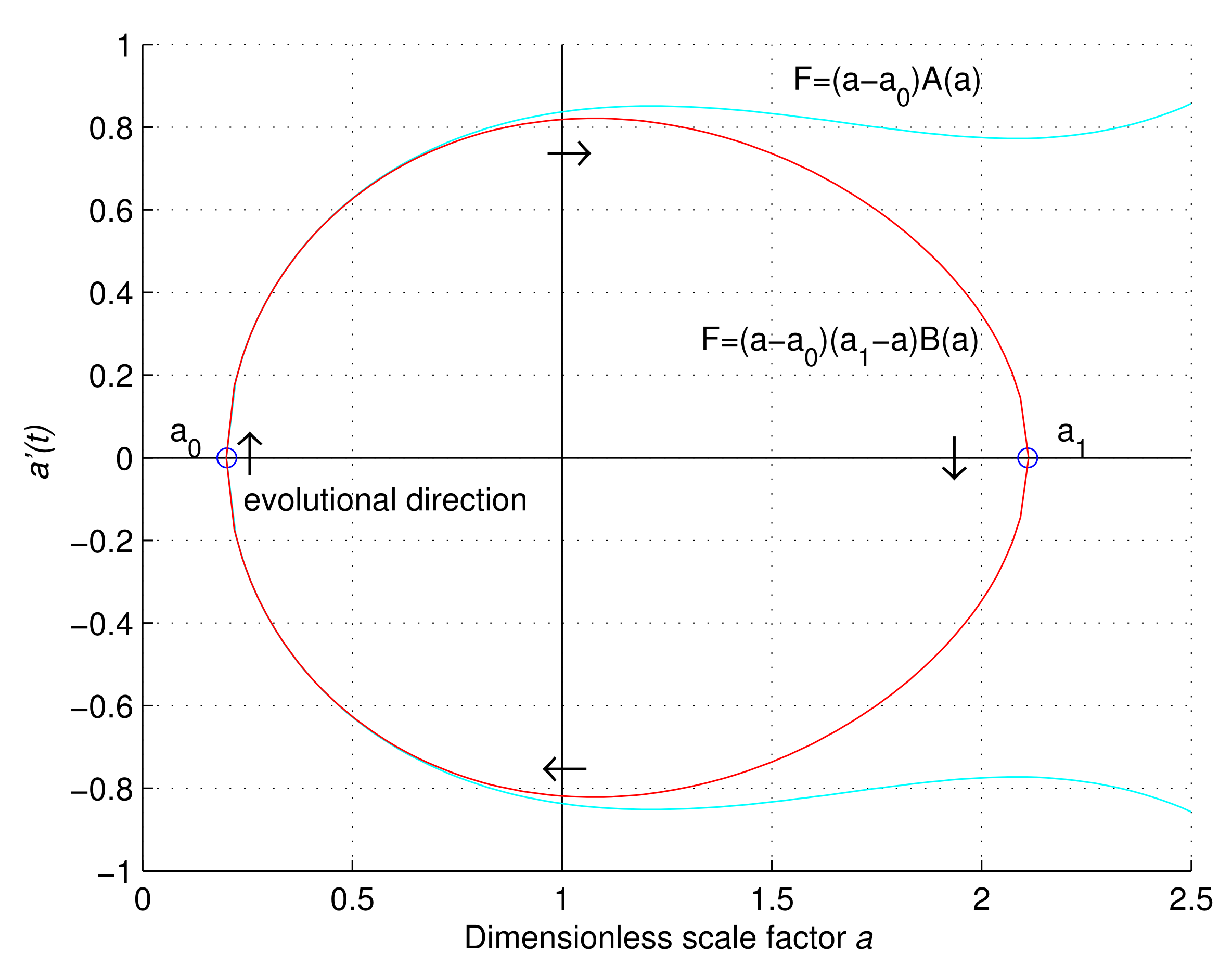
Since Friedmann equation is an equation in average sense, the multiple roots are meaningless in physics. The connected phase trajectories of dynamical Equation (106) with (116) or (117) are displayed in Figure 1, in which we have set the average scale . (117) corresponds to the cyclic cosmological model, and (116) to the bouncing one. We set the time origin at the turning point . Form Figure 1 we learn clearly the initial singularity is absent, i.e., a cannot reaches 0 point.
Since in cosmology, by (117) we certainly have due to . Then we get another conclusion:
, the space of the universe is a closed 3 dimensional sphere.
In the cyclic closed case (117), we have an estimation of upper bound for the cosmological constant . Substituting (117) into (108) and letting , by (43) we have
Since forms the main part of mass-energy density at present time, which can be estimated by observational data [21], and as can be omitted. For we have and estimation
So for the cosmological constant in a cyclic and closed universe, we get the third conclusion:
, the cosmological constant is an infinitesimal.
This estimation is less than the present observational data. This difference can be explained by the potentials W in energy-momentum tensor, which is a fast decaying in Friedmann equation. Therefore setting constant is a good choice in cosmology.
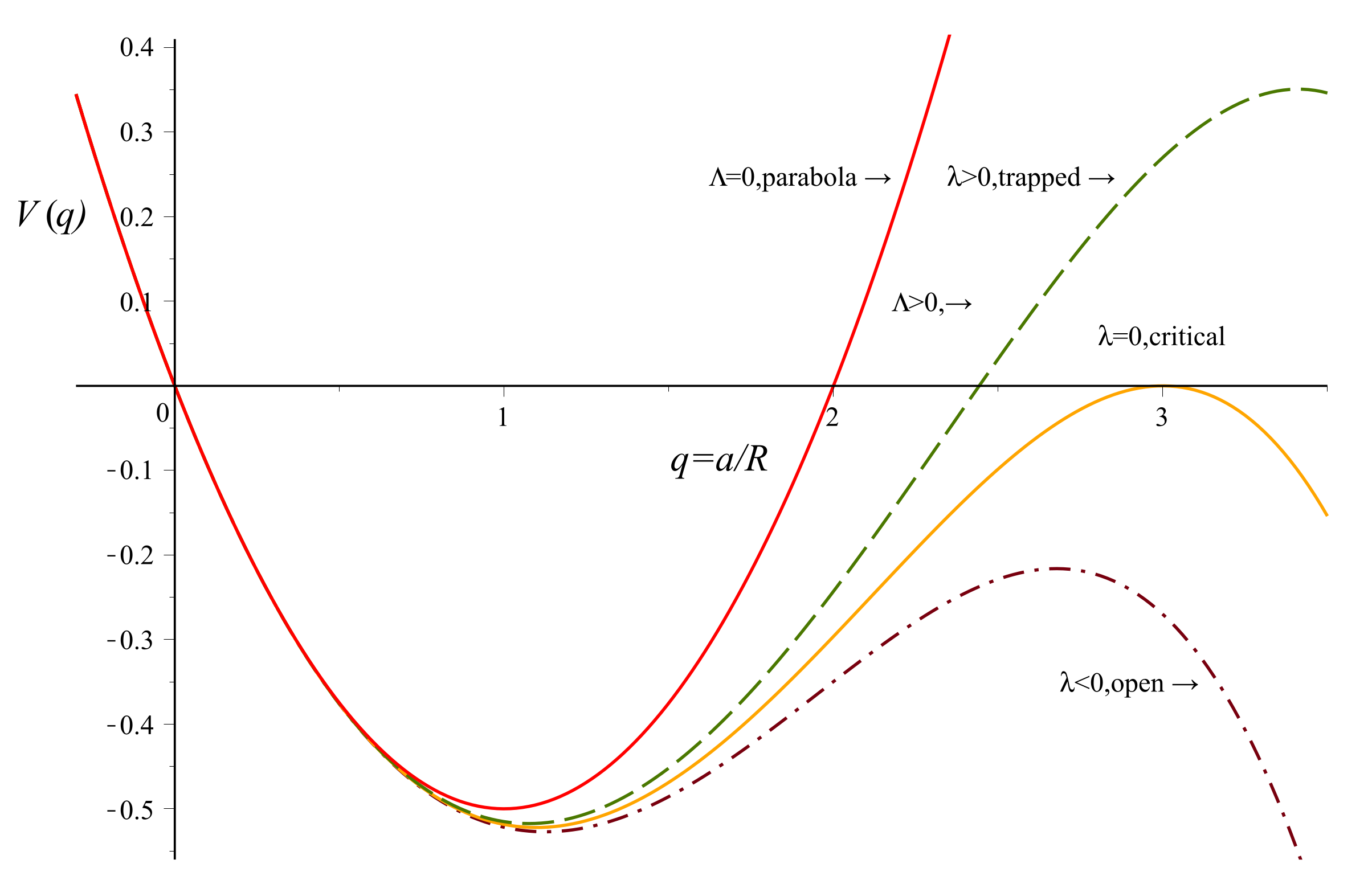
For a bouncing cosmological model, while , the behavior of Friedmann Equation (106) is controlled by dominant term , and the fast decaying term can be omitted. In this case, to be clear, (106) can be replaced by the following dimensionless Hamiltonian-like equation
in which
For solution of Friedmann equation we have , which is conserved.
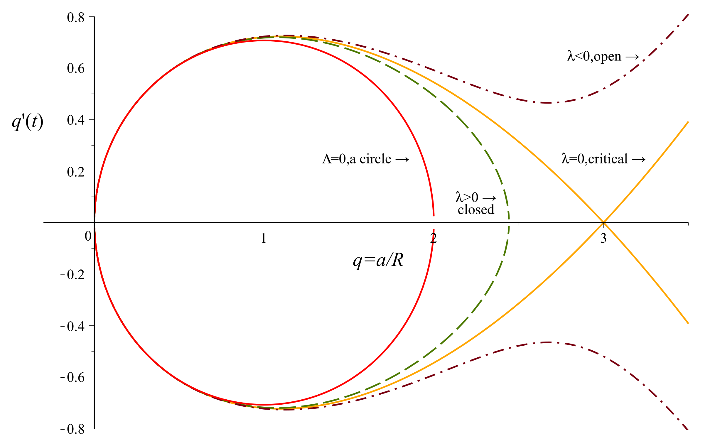
In (121), is equivalent to the coordinate of a unit mass, potential, and H energy. The potential function and phase trajectories is displayed by Figure 2 and Figure 3. The solution is closed if , but bouncing if . As we can see from Figure 2 and Figure 3, or has only influence on the behavior of a fully developed universe but has little influence on a small universe. On the contrary, the function of can prevent from reaching the initial singularity but has little influence on a fully developed universe. For closed universe, we have the second root . In contrast with (120), we find the estimation of by criterion is larger. In bouncing case [25], we have as . In this case, the solution of Friedmann equation globally exists and the asymptotic behavior is controlled by term . For the big rip model, we need an even higher order term in Friedmann equation, which is unreasonable in physics.
The bouncing model with closed space is inconsistent with the isotropy and homogeneity of the present universe, because the universe should be heavily anisotropy and inhomogeneity before the turning point due to the lack of initial causality among remote parts, and some information should be kept today. However, this problem is absent in a cyclic and closed universe, because the anisotropy and inhomogeneity in a period will be polished by the subsequent evolution due to the entropy increasing principle. In a closed system, the dissipative effect will work when the inhomogeneity of the matter distribution is greater than the controlling degree of internal interaction of matter, it reduces the inhomogeneity to match the scale of the interactive force. From the above analysis we find is purely a trouble term without any practical purpose.
5. Towards a Realistic Cosmological Model
In this section, we discuss the cosmological model with nonlinear potentials; that is, we examine the influence of the term on the Friedmann Equations (105)–(109). Based on the analysis of Section 2 and Section 3, we find that in (106), X has an influence on the behavior of the universe at the early age, and only has an influence on the very old universe. has not any clear purpose in physics, so we set . In the conformal coordinate system (104), using (106) and , the dynamics for a cyclic and closed universe is generally given by (105) and (117) as follows
where is the minimum scale and is the maximum scale, are two parameters that reflect the influence of nonlinear potentials on the universe. and the parameters all have length dimension. In fact, (117) only required in the domain . However, is a high order small term and has no influence on the following analysis and calculation, and taking the term adds a lot of cases for judgment, so only the case is needed for the following discussion.
For the convenience of discussion, we define a dimensionless function
For , we have the approximation and in the calculation. The age of the universe is calculated by
where is the present scale of the universe. The solution is the elliptic integrals. Denote the half period of the universe by
By the approximation , we have
where B is defined by
So we have the approximation
In the above calculation, we used , and
then the integral can be calculated.
The Hubble parameter can be calculated as
Denoting the critical density
we have the dimensionless mass density
In the second-order approximation, we find that acts as one parameter and the influence of disappears. This overcomes the shortage of useful observational data. Omitting the higher order terms in (128) and (129), and making the transformation
we obtain 3 equations for 3 parameters .
Theoretically, we can solve for from the above equations using observational data . By (131), we obtain
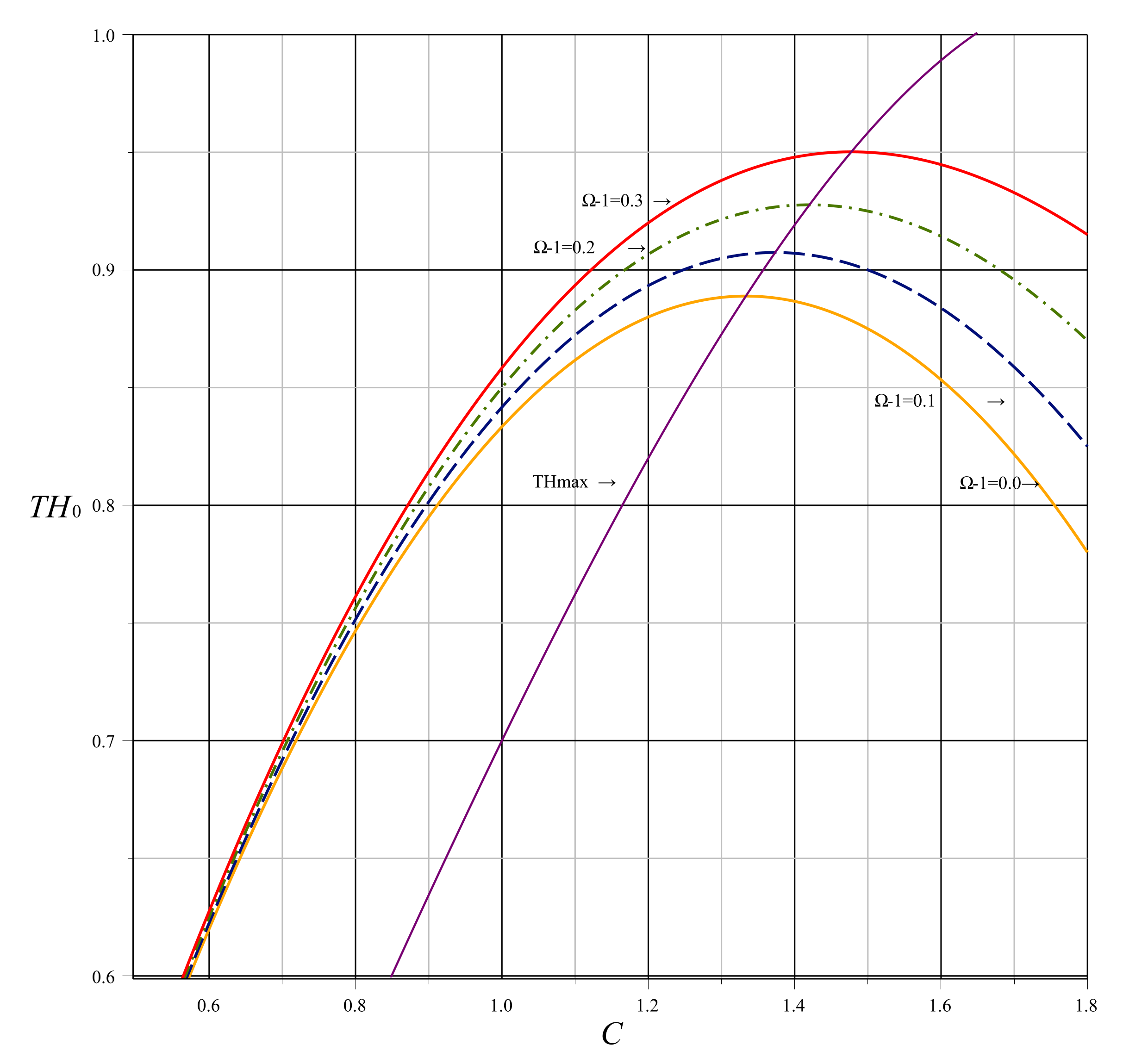
where . Substituting (133) into (132), we obtain the equation for C,
The curves of are displayed in Figure 4. By the definition (130), we find that C is an increasing function of A or , so only the increasing part of the curves are meaningful in physics.
has a maximum. Omitting , we have
For simplicity, we take B as the independent parameter instead of . From (133), we obtain the solution
Substituting it into (134) and noting , we obtain
Substituting it into (135), we obtain C determined by observational data, then by (131), we obtain A. Other parameters can be calculated by
From the observational data set [3,4,5,6], we have the following typical range of parameter values [4],
where h is the dimensionless Hubble parameter
Based on the equations, we calculate the typical values for all parameters, some results are displayed in Table 1.
By calculation, we have
This means that the expansion of the universe is still accelerating. Using (123), we obtain the relation as
Substituting it into (110), we obtain the relation as
From Table 1, we find that the structural parameters are sensitive to mass density : the larger the mass, the smaller the universe, and the rate is very large. The difficulty to detect the little value of is a good news for humanity, as it reflects that the universe is still very young, and we can expect a better future for humanity. Relatively, the parameters are not very sensitive to the age and the Hubble parameter . Since measuring is very difficult and ambiguous, we need a more efficient method to measure cosmic data. Obviously, the above model is hardly contradictory against observational data, this is because the above calculating results are all compatible with observational facts and the effective observational data are still not enough to determine all the coefficients in (123).
The cyclic and closed model can provide more natural explanations for cosmological problems. From (123), we learn that there is a cradle of rebirth rather than an initial singularity. At this time, the drifting speed of the particles or the cosmic temperature takes the maximum, and the volume of the Universe takes the minimum. This situation will result in violent collisions among galaxies and the particles. Such collisions will recover the vitality of the dead stars and combined particles. Besides, the nonlinear potential will become dominant at this time, and the property of the particles will change. Just like the rebirth of the Phoenix, the Universe gets her rebirth at the turning point.
6. Discussion and Conclusions
Since the above derivations are all elementary and reliable, and all concepts have clearly physical meanings, so the conclusions should be quite credible. However, the above conclusions contradict the singularity theorems, this is because some preconditions of these theorems are invalid in physical world [25]. For example, the existence of negative pressure or potential is ignored in the energy condition. Besides, we have only unique realistic simultaneous Cauchy surface in the space-time [30,32], but the derivation of Raychaudhury equation unconsciously assumes and uses the future properties of the space-time. So this equation cannot be generally used for dynamical analysis. A realistic singularity in Nature is actually contradictory and incomprehensible, so the absence of singularity in Nature is a basic principle in physics.
To sum up, by studying the properties of the EMT and EOS of various physical fields, especially the EMT and EOS of nonlinear spinors, and qualitatively analyzing the dynamical behavior of the general Friedmann equation and logical relations between parameters, we get some definite constraints on . We find that only the cyclic and closed cosmological model with a tiny or vanishing is natural and reasonable in physics. The other cases include nonphysical effects or logical contradictions. Such constraints will be helpful for the research of some other issues in cosmology. In some sense, we restored Heraclitus’ ancient faith: “The world, an entity out of everything, was created by neither gods nor men, but was, is and will be eternally living fire, regularly becoming ignited and regularly becoming extinguished”.
Funding
This research received no external funding.
Institutional Review Board Statement
Not applicable.
Informed Consent Statement
Not applicable.
Data Availability Statement
Not applicable.
Acknowledgments
This paper was modified a lot according to the professional suggestions of the two anonymous reviewers, and the Lagrangian of fluid is derived according to the discussion. I sincerely thank them very much.
Conflicts of Interest
The author declares no conflict of interest.
References
- Riess, A.G.; Filippenko, A.V.; Challis, P.; Clocchiatti, A.; Diercks, A.; Garnavich, P.M.; Gilliland, R.L.; Hogan, C.J.; Jha, S.; Kirshner, R.P.; et al. Observational Evidence from Supernovae for an Accelerating Universe and a Cosmological Constant. Astron. J. 1998, 116, 1009. [Google Scholar] [CrossRef]
- Perlmutter, S.; Aldering, G.; Goldhaber, G.; Knop, R.; Nugent, P.; Castro, P.G.; Deustua, S.; Fabbro, S.; Goobar, A.; Groom, D.E.; et al. Measurements of Ω and Λ from 42 High-Redshift Supernovae. Astrophys. J. 1999, 517, 565. [Google Scholar] [CrossRef]
- Spergel, D.N.; Verde, L.; Peiris, H.V.; Komatsu, E.; Nolta, M.; Bennett, C.L.; Halpern, M.; Hinshaw, G.; Jarosik, N.; Kogut, A.; et al. First-Year Wilkinson Microwave Anisotropy Probe (WMAP) Observations: Determination of Cosmological Parameters. Astrophys. J. Suppl. Ser. 2003, 148, 175. [Google Scholar] [CrossRef]
- Tegmark, M.; Strauss, M.A.; Blanton, M.R.; Abazajian, K.; Dodelson, S.; Sandvik, H.; Wang, X.; Weinberg, D.H.; Zehavi, I.; Bahcall, N.A.; et al. Cosmological parameters from SDSS and WMAP. Phys. Rev. 2004, D69, 103501. [Google Scholar] [CrossRef]
- Dunkley, J.; Hlozek, R.; Sievers, J.; Acquaviva, V.; Ade, P.A.; Aguirre, P.; Amiri, M.; Appel, J.W.; Barrientos, L.F.; Battistelli, E.S.; et al. The Atacama Cosmology Telescope: Cosmological Parameters from the 2008 Power Spectra. Astrophys. J. 2011, 739, 52. [Google Scholar] [CrossRef]
- Sievers, J.L.; Hlozek, R.A.; Nolta, M.R.; Acquaviva, V.; Addison, G.E.; Ade, P.A.; Aguirre, P.; Amiri, M.; Appel, J.W.; Barrientos, L.F.; et al. The Atacama Cosmology Telescope: Cosmological parameters from three seasons of data. JCAP 2013, 10, 60. [Google Scholar] [CrossRef]
- Sahni, V. The cosmological constant problem and quintessence. Class. Quant. Gravity 2002, 19, 3435–3448. [Google Scholar] [CrossRef]
- Peebles, P.J.E.; Ratra, B. The Cosmological Constant and Dark Energy. Rev. Mod. Phys. 2003, 75, 559–606. [Google Scholar] [CrossRef]
- Turner, M.S.; Huterer, D. Cosmic Acceleration, Dark Energy and Fundamental Physics. J. Phys. Soc. Jpn. 2007, 76, 111015. [Google Scholar] [CrossRef]
- Ishak, M. Remarks on the formulation of the cosmological constant/dark energy problems. Found. Phys. 2007, 37, 1470–1498. [Google Scholar] [CrossRef]
- Szydlowski, M.; Kurek, A.; Krawiec, A. Top ten accelerating cosmological models. Phys. Lett. B 2006, 642, 171–178. [Google Scholar] [CrossRef]
- Szydlowski, M. Cosmological zoo—Accelerating models with dark energy. JCAP 2007, 0709, 7. [Google Scholar] [CrossRef]
- Copeland, E.J.; Sami, M.; Tsujikawa, S. Dynamics of dark energy. IJMPD 2006, 15, 1753–1936. [Google Scholar] [CrossRef]
- Linder, E.V. Theory Challenges of the Accelerating Universe. J. Phys. A 2007, 40, 6697. [Google Scholar] [CrossRef][Green Version]
- Bull, P.; Akrami, Y.; Adamek, J.; Baker, T.; Bellini, E.; Jimenez, J.B.; Bentivegna, E.; Camera, S.; Clesse, S.; Davis, J.H.; et al. Beyond ΛCDM: Problems, solutions, and the road ahead. Phys. Dark Universe 2016, 12, 56–99. [Google Scholar] [CrossRef]
- Steinhardt, P.J.; Turok, N. A Cyclic Model of the Universe. Science 2002, 296, 1436. [Google Scholar] [CrossRef] [PubMed]
- Steinhardt, P.J.; Turok, N. The Cyclic Model Simplified. New Astron. Rev. 2005, 49, 43–57. [Google Scholar] [CrossRef]
- Khoury, J.; Steinhardt, P.J.; Turok, N. Designing Cyclic Universe Models. Phys. Rev. Lett. 2004, 92, 031302. [Google Scholar] [CrossRef] [PubMed]
- Barrow, J.D.; Dabrowski, M.P. Oscillating universes. Mon. Not. Astron. Soc. 1995, 275, 850–862. [Google Scholar] [CrossRef]
- Barrow, J.D.; Kimberly, D.; Magueijo, J. Bouncing Universes with Varying Constants. Class. Quant. Gravity 2013, 21, 57–61. [Google Scholar] [CrossRef]
- Gu, Y.Q. A Cosmological Model with Dark Spinor Source. Int. J. Mod. Phys. 2007, A22, 4667–4678. [Google Scholar] [CrossRef]
- Gu, Y.Q. Clifford Algebra, Lorentz Transformation and Unified Field Theory. Adv. Appl. Clifford Algebras 2018, 28, 37. [Google Scholar] [CrossRef]
- Madsen, M.; Ellis, G. The evolution of Ω in inflationary universes. Mon. Not. R. Astron. Soc. 1988, 234, 67–77. [Google Scholar] [CrossRef][Green Version]
- Ellis, G.F.; Platts, E.; Sloan, D.; Weltman, A. Current observations with a decaying cosmological constant allow for chaotic cyclic cosmology. JCAP 2016, 4, 26. [Google Scholar] [CrossRef]
- Novello, M.; Bergliaffa, S.E.P. Bouncing Cosmologies. Phys. Rep. 2008, 463, 127–213. [Google Scholar] [CrossRef]
- Di Valentino, E. Melchiorri, A.; Silk, J. Planck evidence for a closed Universe and a possible crisis for cosmology. Nat. Astron. 2020, 4, 196–203. [Google Scholar] [CrossRef]
- Gu, Y.Q. Dynamic Behavior and Topological Structure of the Universe with Dark Energy. arXiv 2007, arXiv:0709.2414. [Google Scholar]
- Gu, Y.Q. Some Applications of Clifford Algebra in Geometry; Shah, K., Lei, M., Eds.; Chapter 4 in Structure Topology and Symplectic Geometry; IntechOpen Limited: London, UK, 2021. [Google Scholar]
- Nester, J.M. Special orthonormal frames. J. Math. Phys. 1992, 33, 910. [Google Scholar] [CrossRef]
- Gu, Y.Q. Theory of Spinors in Curved Space-Time. Symmetry 2021, 13, 1931. [Google Scholar] [CrossRef]
- Gu, Y.Q. Clifford Algebra and Unified Field Theory (Ch.7.2, Ch.8.3, Ch.9.2); LAP LAMBERT Academic Publishing: Chisinau, Moldova, 2020; Available online: www.morebooks.shop/store/gb/book/clifford-algebra-and-unified-field-theory/isbn/978-620-2-81504-8 (accessed on 16 September 2020).
- Gu, Y.Q. Natural Coordinate System in Curved Space-time. J. Geom. Symmetry Phys. 2018, 47, 51–62. [Google Scholar] [CrossRef]
- Weinberg, S.L. Gravitation and Cosmology (Ch.11); Wiley: New York, NY, USA, 1972. [Google Scholar]
- Ozer, M.; Taha, M.O. A Possible Solution to the Main Cosmological Problems. Phys. Lett. B 1986, 171, 363–365. [Google Scholar] [CrossRef]
- Ozer, M.; Taha, M.O. A Model of the Universe Free of Cosmological Problems. Nuclear Phys. B 1987, 287, 776–796. [Google Scholar] [CrossRef]
- Chen, W.; Wu, Y. Implications of a Cosmological Constant Varying as R-2. Phys. Rev. 1990, 41, 695–698. [Google Scholar] [CrossRef]
- Berman, M. Cosmological Models with a Variable Cosmological Term. Phys. Rev. D 1991, 43, 1075–1078. [Google Scholar] [CrossRef]
- Al-Rawaf, A.S.; Taha, M.O. Cosmology of General Relativity without Energy-Momentum Conservation. Gen. Rel. Gravity 1996, 28, 935–952. [Google Scholar] [CrossRef]
- Al-Rawaf, A.S. A Cosmological Model with a Generalized Cosmological Constant. Mod. Phys. Lett. A 1998, 13, 429–432. [Google Scholar] [CrossRef]
- Overduin, J.M.; Cooperstock, F.I. Evolution of the Scale Factor with a Variable Cosmological Term. Phys. Rev. D 1998, 58, 043506. [Google Scholar] [CrossRef]
- Arbab, A.I. Cosmic Acceleration with a Positive Cosmological Constant. Class. Quant. Gravity 2003, 28, 93–99. [Google Scholar] [CrossRef]
- Gu, Y.Q. Simplification of Galactic Dynamic Equations. Available online: www.preprints.org (accessed on 27 February 2020).
- Barrow, J.D. Finite Action Principle Revisited. Phys. Rev. D 2020, 101, 023527. [Google Scholar] [CrossRef]
- Gu, Y.Q. Local Lorentz Transformation and Mass-Energy Relation of Spinor. Phys. Essays 2018, 31, 1–6. [Google Scholar] [CrossRef]
Figure 1.
The phase trajectories of Friedmann Equation (106).
Figure 1.
The phase trajectories of Friedmann Equation (106).

Figure 2.
Potential defined in (121).
Figure 2.
Potential defined in (121).

Figure 3.
Phase trajectories of similar to Figure 1. Inside the circle and outside . In Friedmann Equation (106), removes the Big Bang.

Figure 4.
The relation among . Only the increasing part is reasonable in physics.


Table 1.
Correlation Among Cosmic Parameters.
| Equation (129) | 0.00010 | 0.0010 | 0.0025 | 0.0050 | 0.0050 | 0.0075 | 0.0003 | |
| , Gyr | Cosmic Age | 12.0000 | 12.000 | 13.000 | 13.000 | 11.000 | 11.000 | 12.000 |
| h | Hubble’s | 0.60000 | 0.6000 | 0.6500 | 0.6500 | 0.7000 | 0.7500 | 0.7000 |
| , 1/Gyr | Hubble’s | 0.06138 | 0.0614 | 0.0665 | 0.0665 | 0.0716 | 0.0767 | 0.0716 |
| Equation (131) | 0.73656 | 0.7366 | 0.8644 | 0.8644 | 0.7877 | 0.8440 | 0.8593 | |
| B | Equation (136) | 0.00671 | 0.0212 | 0.0364 | 0.0515 | 0.0486 | 0.0618 | 0.0114 |
| C | Equation (135) | 0.78137 | 0.7813 | 1.1110 | 1.1097 | 0.8828 | 1.0314 | 1.0900 |
| A, Gly | Present Scale | 948.07 | 299.78 | 229.56 | 162.14 | 126.82 | 108.83 | 665.23 |
| , Gly | Equation (137) | 1155.35 | 365.34 | 204.09 | 144.35 | 141.68 | 105.42 | 605.33 |
| , Gly | Largest Scale | 21,035,047 | 665,393 | 173,573 | 61,381 | 53,810 | 28,643 | 5,082,600 |
| , Gyr | Half Period | 33,043,667 | 1,045,773 | 272,969 | 96,644 | 84,747 | 45,157 | 7,984,698 |
Publisher’s Note: MDPI stays neutral with regard to jurisdictional claims in published maps and institutional affiliations. |
© 2021 by the author. Licensee MDPI, Basel, Switzerland. This article is an open access article distributed under the terms and conditions of the Creative Commons Attribution (CC BY) license (https://creativecommons.org/licenses/by/4.0/).
Share and Cite
MDPI and ACS Style
Gu, Y.-Q. Dynamical Reason for a Cyclic Universe. Symmetry 2021, 13, 2272. https://doi.org/10.3390/sym13122272
AMA Style
Gu Y-Q. Dynamical Reason for a Cyclic Universe. Symmetry. 2021; 13(12):2272. https://doi.org/10.3390/sym13122272
Chicago/Turabian StyleGu, Ying-Qiu. 2021. "Dynamical Reason for a Cyclic Universe" Symmetry 13, no. 12: 2272. https://doi.org/10.3390/sym13122272
APA StyleGu, Y.-Q. (2021). Dynamical Reason for a Cyclic Universe. Symmetry, 13(12), 2272. https://doi.org/10.3390/sym13122272
Note that from the first issue of 2016, this journal uses article numbers instead of page numbers. See further details here.