A Proximal Algorithm with Convergence Guarantee for a Nonconvex Minimization Problem Based on Reproducing Kernel Hilbert Space

Abstract

The underlying function in reproducing kernel Hilbert space (RKHS) may be degraded by outliers or deviations, resulting in a symmetry ill-posed problem. This paper proposes a nonconvex minimization model with ${\ell }_0$-quasi norm based on RKHS to depict this degraded problem. The underlying function in RKHS can be represented by the linear combination of reproducing kernels and their coefficients. Thus, we turn to estimate the related coefficients in the nonconvex minimization problem. An efficient algorithm is designed to solve the given nonconvex problem by the mathematical program with equilibrium constraints (MPEC) and proximal-based strategy. We theoretically prove that the sequences generated by the designed algorithm converge to the nonconvex problem’s local optimal solutions. Numerical experiment also demonstrates the effectiveness of the proposed method.

1. Introduction

The reproducing kernel Hilbert space (RKHS, denote as $\mathcal{H}$) has been widely studied in many studies [1,2,3,4,5,6,7]. Its most critical property is that the functions in RKHS can be linearly represented by reproducing kernel function. In addition, many studies have analyzed the properties of unitary or binary functions in RKHS. These functions usually can be regarded as signals or images in discrete form, so as to build optimization models and solve some application problems, such as image super-resolution and image restoration.

In general, the Hilbert space can be considered as $\mathcal{H}\subset L^2\left(\mathbb{P}\right)$ which $\mathbb{P}$ is a probability measure on the subset $\mathcal{X}\subset \mathbb{R}$, $\mathcal{H}$ is complete for a class of real valued functions $f:\mathcal{X}\to \mathbb{R}$ with ${\parallel f\parallel }_{L^2\left(\mathbb{P}\right)}<\infty$. Moreover, the reproducing kernel $\kappa$ of $\mathcal{H}$ can be defined as: (1) for any $x\in \mathcal{X}$, the function $\kappa (·,x)$ blongs to $\mathcal{H}$. (2) the function $\kappa$ has so-called reproducing property, that is $f\left(x\right)={⟨f,\kappa (·,x)⟩}_{\mathcal{H}}$ for all $f\in \mathcal{H}$, and ${⟨·,·⟩}_{\mathcal{H}}$ represents an associated inner product. By this relation, we could get the Gram matrix $\mathbf{K}\in {\mathbb{R}}^{n\times n}$ by the discretization of reproducing kernel $\kappa (·,\mathbf{x})$ for $\mathbf{x}\in {\mathbb{R}}^n$, thus it is easy to get the following discrete formulation by considering the bias $\mathbf{e}\in {\mathbb{R}}^n$:

$$\begin{array}{c}\hfill \mathbf{g}=\mathbf{K}\mathbf{\alpha }+\mathbf{e},\end{array}$$

(1)

where $\mathbf{\alpha }\in {\mathbb{R}}^n$ is the coefficient we need to estimate, besides, $\mathbf{K}$ is a real symmetry matrix.

In the real world, the underlying function $\mathbf{g}$ generally will be polluted by outliers and Gaussian perturbation, which gets the following symmetry ill-posed problem:

$$\begin{array}{c}\hfill \mathbf{y}=\mathbf{K}\mathbf{\alpha }+\mathbf{e}+\mathbf{u}+\mathbf{\sigma },\end{array}$$

(2)

where $\mathbf{u}\in {\mathbb{R}}^n$ can be viewed as outliers and $\mathbf{\sigma }\in {\mathbb{R}}^n$ stands for Gaussian perturbation. Our final goal is to accurately estimate the coefficients $\mathbf{\alpha }$ and $\mathbf{e}$ from the known $\mathbf{y}$ and $\mathbf{K}$. After obtaining $\mathbf{\alpha }$ and $\mathbf{e}$, we could calculate the underlying function $\mathbf{g}$ by (1). Note that, solving the problem (2) is quite a chanllenging task, since the variables $\mathbf{\alpha }$, $\mathbf{e}$, $\mathbf{u}$ and $\mathbf{\sigma }$ in (2) are all unknown, which leads to a ill-posed problem.

In [8], Papageorfiou et al, considered that the function g can be linearly represented by coefficient $\alpha$ and constant c as $\mathbf{g}=\mathbf{K}\mathbf{\alpha }+c\mathbf{1}$, and proposed a kernel regularized orthogonal maching pursuit (KROMP) method to solve the nonconvex problem. However, the KROMP method has two weakness: one is that the constant c is not general and flexible; the other is that the convergence of its algorithm is not guaranteed theoretically. Therefore, this paper mainly establishes the nonconvex optimization model for the degraded problem (2) in RKHS, and gives the designed algorithm whose convergence can be guaranteed, finally shows the effectiveness of the proposed method in some simulation experiments.

Regularized modeling is a promising way to deal with ill-posed problems. Actually, the variable $\mathbf{u}$ representing outliers is generally sparse, which motivates us to formulate a sparsity-based regularization model. Especially, ${\ell }_0$-quasi norm that counts the non-zero elements in a vector is an ideal metric to depict the sparse property. Therefore, the nonconvex minimization problem for solving the ill-posed problem (2) can be simply shown as follows,

$$\begin{array}{c}\hfill \underset{\mathbf{\alpha },\mathbf{e},\mathbf{u}\in {\mathbb{R}}^n}{min}\mathsf{\Phi }(\mathbf{\alpha },\mathbf{e},\mathbf{u})=\frac{\mu }{2}{\parallel \mathbf{K}\mathbf{\alpha }+\mathbf{e}+\mathbf{u}-\mathbf{y}\parallel }_2^2+\frac{{\lambda }_1}{2}{\parallel \mathbf{\alpha }\parallel }_2^2+\frac{{\lambda }_2}{2}{\parallel \mathbf{e}\parallel }_2^2+{\parallel \mathbf{u}\parallel }_0,\end{array}$$

(3)

where $\mu$, ${\lambda }_1$ and ${\lambda }_2$ are positive parameters. The first term in (3) is deduced from the Gaussian perturbation of $\mathbf{\sigma }$ under the framework of maximum a posteriori (MAP) estimation. The second and third terms are two regularized terms to depict the underlying prior for $\mathbf{\alpha }$ and $\mathbf{e}$. The last term is a ${\ell }_0$-quasi norm to depict the sparse prior of outlier $\mathbf{u}$. Note that the given regularization model (3) is a nonconvex minimization problem due to the nonconvex property of ${\ell }_0$ term. In general, the ${\ell }_0$ term will be replaced approximately by some other convex terms (e.g., ${\ell }_1$ term or hard threshold [9,10,11,12]) for simpler computation and convergence guarantee. However, if taking this way, it will lose the accuracy of depicting sparsity, which may result in unreasonable outcomes.

However, the nonconvex minimization problems usually have the following difficulties which are encountered to solve: (1) Whether the designed algorithm can effectively solve the minimization model? (2) Whether the convergence analysis of the designed algorithm can be guaranteed? (3) Whether the initial value affects the convergence of the designed algorithm? Thus, many studies have been devote to conquer these weaknesses of nonconvex problems.

Recently, the nonconvex problem can be reformulated as an equivalent minimization problem based on the mathematical program with equilibrium constraints (MPEC) which can be effectively solved by the classical algorithms [13,14,15]. For instance, Yuan et al. [14] have proposed an equivalent biconvex MPEC formulation for ${\ell }_0$-quasi norm of the nonconvex minimization problem. Additionally, the proximal alternating based algorithm has widely been used to solve the nonconvex and nonsmooth problems [16,17,18,19,20,21,22,23,24]. In [18], Bolte et al. propose a proximal alternating linear minimization algorithm (PALM) framework to solve nonconvex and nonsmoothing minimization problem, and give the convergence analysis of the algorithm.

In this paper, we mainly focus on the above mentioned difficulties of nonconvex minimization problem (3) to design an efficient algorithm with convergence guarantee theoretically. A simple and representative example is employed to verify the effectiveness of the proposed method. Besides, the contributions of this work can be summarized as: (1) New nonconvex minimization modeling based on RKHS; (2) Convergence guarantee of the designed algorithm for the nonconvex problem.

The outline of this paper is as follows. Section 2 shows the detailed algorithm for the nonconvex minimization problem (3). In Section 3, the convergence analysis of the given algorithm is given. Numerical results are reported in Section 4. Finally, conclusions are drawn in Section 5.

2. The Solution for the Nonconvex Minimization Problem

Based on the MPEC lemma of ${\ell }_0$-quasi norm (see more details from [14]), the nonconvex minimization problem (3) can be equivalently reformulated the following model:

$$\begin{array}{cc}\hfill \underset{\mathbf{\alpha },\mathbf{e},\mathbf{u},\mathbf{v}\in {\mathbb{R}}^n}{min}& \mathsf{\Phi }(\mathbf{\alpha },\mathbf{e},\mathbf{u},\mathbf{v})=\frac{\mu }{2}{\parallel \mathbf{K}\mathbf{\alpha }+\mathbf{e}+\mathbf{u}-\mathbf{y}\parallel }_2^2+\frac{{\lambda }_1}{2}{\parallel \mathbf{\alpha }\parallel }_2^2+\frac{{\lambda }_2}{2}{\parallel \mathbf{e}\parallel }_2^2\hfill \\ \hfill & +⟨\mathbf{1},\mathbf{1}-\mathbf{v}⟩+{\iota }_{[0,1]}\left(\mathbf{v}\right)\hfill \\ \hfill & s.t.\mathbf{v}\odot \left|\mathbf{u}\right|=0,\hfill \end{array}$$

(4)

where ⊙ represents point-wise multiplication, and ${\iota }_{[0,1]}\left(\mathbf{v}\right)$ is indicator function projecting the elements of $\mathbf{v}$ into $[0,1]$. The constrained minimization problem (4) can be rewritten as the following unconstrained minimization problem by the penalty strategy:

$$\begin{array}{c}\hfill \mathsf{\Phi }(\mathbf{\alpha },\mathbf{e},\mathbf{u},\mathbf{v})=H(\mathbf{\alpha },\mathbf{e},\mathbf{u},\mathbf{v})+f_1\left(\mathbf{\alpha }\right)+f_2\left(\mathbf{e}\right)+f_3\left(\mathbf{u}\right)+f_4\left(\mathbf{v}\right),\end{array}$$

(5)

where $H(\mathbf{\alpha },\mathbf{e},\mathbf{u},\mathbf{v})=\frac{\mu }{2}{\parallel \mathbf{K}\mathbf{\alpha }+\mathbf{e}+\mathbf{u}-\mathbf{y}\parallel }_2^2+\frac{\beta }{2}{\parallel \mathbf{v}\odot \left|\mathbf{u}\right|\parallel }_2^2$, $f_1\left(\mathbf{\alpha }\right)=\frac{{\lambda }_1}{2}{\parallel \mathbf{\alpha }\parallel }_2^2$, $f_2\left(\mathbf{e}\right)=\frac{{\lambda }_2}{2}{\parallel \mathbf{e}\parallel }_2^2$, $f_3\left(\mathbf{u}\right)=0$, $f_4\left(\mathbf{v}\right)=⟨\mathbf{1},\mathbf{1}-\mathbf{v}⟩+{\iota }_{[0,1]}\left(\mathbf{v}\right)$.

We utilize the proximal-based algorithm to effectively deal with the unconstrained problem (5) by alternatingly solving each variable, which leads to the following subproblems:

$$\begin{array}{cc}\hfill {\mathbf{\alpha }}^{k+1}& \in arg\underset{\mathbf{\alpha }}{min}⟨\mathbf{\alpha }-{\mathbf{\alpha }}^k,{\partial }_{\mathbf{\alpha }}H({\mathbf{\alpha }}^k,{\mathbf{e}}^k,{\mathbf{u}}^k,{\mathbf{v}}^k)⟩+f_1\left(\mathbf{\alpha }\right)+\frac{{\tau }_1}{2}{\parallel \mathbf{\alpha }-{\mathbf{\alpha }}^k\parallel }_2^2,\hfill \end{array}$$

(6)

$$\begin{array}{cc}\hfill {\mathbf{e}}^{k+1}& \in arg\underset{\mathbf{e}}{min}⟨\mathbf{e}-{\mathbf{e}}^k,{\partial }_{\mathbf{e}}H({\mathbf{\alpha }}^{k+1},{\mathbf{e}}^k,{\mathbf{u}}^k,{\mathbf{v}}^k)⟩+f_2\left(\mathbf{e}\right)+\frac{{\tau }_2}{2}{\parallel \mathbf{e}-{\mathbf{e}}^k\parallel }_2^2,\hfill \end{array}$$

(7)

$$\begin{array}{cc}\hfill {\mathbf{u}}^{k+1}& \in arg\underset{\mathbf{u}}{min}H({\mathbf{\alpha }}^{k+1},{\mathbf{e}}^{k+1},\mathbf{u},{\mathbf{v}}^k)+f_3\left(\mathbf{u}\right)+\frac{{\delta }_1}{2}{\parallel \mathbf{u}-{\mathbf{u}}^k\parallel }_2^2,\hfill \end{array}$$

(8)

$$\begin{array}{cc}\hfill {\mathbf{v}}^{k+1}& \in arg\underset{\mathbf{v}}{min}H({\mathbf{\alpha }}^{k+1},{\mathbf{e}}^{k+1},{\mathbf{u}}^{k+1},\mathbf{v})+f_4\left(\mathbf{v}\right)+\frac{{\delta }_2}{2}{\parallel \mathbf{v}-{\mathbf{v}}^k\parallel }_2^2,\hfill \end{array}$$

(9)

where the related parameters are all nonnegative, i.e., ${\delta }_1>0,{\delta }_2>0$, and ${\tau }_1={\gamma }_1{\parallel {\mathbf{K}}^T\mathbf{K}\parallel }_F$, ${\tau }_2={\gamma }_2{\parallel {\mathbf{I}}_m^T{\mathbf{I}}_m\parallel }_F$, here ${\mathbf{I}}_m\in {\mathbb{R}}^{m\times m}$ is identity matrix, and ${\parallel ·\parallel }_F$ represents Frobenius norm, ${\gamma }_1>1$, ${\gamma }_2>1$.

In particular, above subproblems are all convex functions whose closed-form solutions can be easily calculated as follows:

$$\begin{array}{c}\hfill {\mathbf{\alpha }}^{k+1}={({\lambda }_1+{\tau }_1)}^{-1}\left(\mu {\mathbf{K}}^T(\mathbf{y}-\mathbf{K}{\mathbf{\alpha }}^k-{\mathbf{e}}^k-{\mathbf{u}}^k)+{\tau }_1{\mathbf{\alpha }}^k\right),\end{array}$$

(10)

$$\begin{array}{c}\hfill {\mathbf{e}}^{k+1}={({\lambda }_2+{\tau }_2)}^{-1}\left(\mu \left(\mathbf{y}-\mathbf{K}{\mathbf{\alpha }}^{k+1}-{\mathbf{e}}^k-{\mathbf{u}}^k\right)+{\tau }_2{\mathbf{e}}^k\right),\end{array}$$

(11)

$$\begin{array}{c}\hfill {\mathbf{u}}^{k+1}=\frac{\mu (\mathbf{y}-\mathbf{K}{\mathbf{\alpha }}^{k+1}-{\mathbf{e}}^{k+1})+{\delta }_1{\mathbf{u}}^k}{\mu +\beta {\mathbf{v}}^k\odot {\mathbf{v}}^k+{\delta }_1},\end{array}$$

(12)

$$\begin{array}{c}\hfill {\mathbf{v}}^{k+1}=min\left(1,max\left(0,\frac{\mathbf{1}+{\delta }_2{\mathbf{v}}^k}{\beta {\mathbf{u}}^{k+1}\odot {\mathbf{u}}^{k+1}+{\delta }_2}\right)\right).\end{array}$$

(13)

We iteratively and alternatingly update ${\mathbf{\alpha }}^{k+1}$, ${\mathbf{e}}^{k+1}$, ${\mathbf{u}}^{k+1}$ and ${\mathbf{v}}^{k+1}$ according to (10)–(13). The final algorithm for the nonconvex minimization problem (3) is summarized in Algorithm 1.

In Algorithm 1, “${\mathrm{Max}}_{iter}$” means the maximum iterations and the “$rho$” represents the relative error between adjacent iterations. When the iteration stops, the final underlying function can be estimated by the relation of (1).

Algorithm 1: The algorithm to minimize the problem (5)

Input: blurred matrix $\mathbf{K}$, positive parameters ${\lambda }_1$, ${\lambda }_2$, ${\delta }_1$${\delta }_2$,           and ${\gamma }_1>1$, ${\gamma }_2>1$. Initialize: start with any $({\mathbf{\alpha }}^0,{\mathbf{e}}^0,{\mathbf{u}}^0,{\mathbf{v}}^0)$, $rho=1$, $k=0$. While$k<{\mathrm{Max}}_{iter}$ or $rho>{10}^{-4}$       (1) Compute ${\mathbf{\alpha }}^{k+1}$ solved by Equation (10).       (2) Compute ${\mathbf{e}}^{k+1}$ by Equation (11).       (3) Compute ${\mathbf{u}}^{k+1}$ by Equation (12).       (4) Compute ${\mathbf{v}}^{k+1}$ by Equation (13).       (5) Update penalty parameter $\beta$ by ${\beta }^{k+1}=1.1{\beta }^k$.       (6) Calculate the relative error $rho=\frac{\parallel {\mathbf{g}}^{k+1}-{\mathbf{g}}^k{\parallel }_2}{\parallel {\mathbf{g}}^k{\parallel }_2}$,            where ${\mathbf{g}}^{k+1}=\mathbf{K}{\mathbf{\alpha }}^{k+1}+{\mathbf{e}}^{k+1}$, and ${\mathbf{g}}^k=\mathbf{K}{\mathbf{\alpha }}^k+{\mathbf{e}}^k$.       (7) $k\leftarrow k+1$. Endwhile Output:${\mathbf{\alpha }}^{*}$, and ${\mathbf{e}}^{*}$

3. Convergence Analysis

For the sake of notational simplicity, we uniform expression $\parallel *\parallel$ as: (1) Frobenius norm ${\parallel *\parallel }_F$ if ∗ is a matrix; (2) ${\ell }_2$-norm ${\parallel *\parallel }_2$ if * is a vector. Denote that ${\mathbf{z}}^k=({\mathbf{\alpha }}^k,{\mathbf{e}}^k,{\mathbf{u}}^k,{\mathbf{v}}^k)$ and its domain field is ${\mathbb{R}}^n\times {\mathbb{R}}^n\times {\mathbb{R}}^n\times {\mathbb{R}}^n$.

Lemma 1.

Let the bounded sequence${\left\{{\mathbf{z}}^k\right\}}_{k\in \mathbb{N}}$is generated by designed algorithm. Then the sequence${\left\{\mathsf{\Phi }\left({\mathbf{z}}^k\right)\right\}}_{k\in \mathbb{N}}$sufficiently decreases as follows:

$$\begin{array}{c}\hfill \mathsf{\Phi }\left({\mathbf{z}}^k\right)-\mathsf{\Phi }\left({\mathbf{z}}^{k+1}\right)\ge \frac{{\rho }_1}{2}{\parallel {\mathbf{z}}^{k+1}-{\mathbf{z}}^k\parallel }^2,\end{array}$$

(14)

where${\rho }_1=min\{\frac{{\tau }_1-L_1}{2},\frac{{\tau }_2-L_2}{2},\frac{{\delta }_1}{2},\frac{{\delta }_2}{2}\}$. Note that${\tau }_1-L_1>0$,${\tau }_1-L_1>0$, and$L_1$is Lipschitz constant of${\partial }_{\mathbf{\alpha }}H$for$\mathbf{\alpha }$, and$L_2$is that of${\partial }_{\mathbf{e}}H$for$\mathbf{e}$.

Proof. 

Since $H(\mathbf{\alpha },\mathbf{e},\mathbf{u},\mathbf{v})$ is Lipschitz differential for variables $\mathbf{\alpha }$ and $\mathbf{e}$, respectively. There exist positive constants $L_1$ and $L_2$ which satisfy:

$$\begin{array}{cc}\hfill H({\mathbf{\alpha }}^{k+1},{\mathbf{e}}^k,{\mathbf{u}}^k,{\mathbf{v}}^k)\le & H({\mathbf{\alpha }}^k,{\mathbf{e}}^k,{\mathbf{u}}^k,{\mathbf{v}}^k)+⟨{\mathbf{\alpha }}^{k+1}-{\mathbf{\alpha }}^k,{\partial }_{\mathbf{\alpha }}H({\mathbf{\alpha }}^k,{\mathbf{e}}^k,{\mathbf{u}}^k,{\mathbf{v}}^k)⟩\hfill \\ \hfill & +\frac{L_1}{2}{\parallel {\mathbf{\alpha }}^{k+1}-{\mathbf{\alpha }}^k\parallel }^2,\hfill \end{array}$$

(15)

$$\begin{array}{cc}\hfill H({\mathbf{\alpha }}^{k+1},{\mathbf{e}}^{k+1},{\mathbf{u}}^k,{\mathbf{v}}^k)\le & H({\mathbf{\alpha }}^{k+1},{\mathbf{e}}^k,{\mathbf{u}}^k,{\mathbf{v}}^k)+⟨{\mathbf{e}}^{k+1}-{\mathbf{e}}^k,{\partial }_{\mathbf{e}}H({\mathbf{\alpha }}^{k+1},{\mathbf{e}}^k,{\mathbf{u}}^k,{\mathbf{v}}^k)⟩\hfill \\ \hfill & +\frac{L_2}{2}{\parallel {\mathbf{e}}^{k+1}-{\mathbf{e}}^k\parallel }^2.\hfill \end{array}$$

(16)

$\mathbf{\alpha }$-subproblem: Based on the designed algorithm, ${\mathbf{\alpha }}^{k+1}$ is the minimum solution of $\mathbf{\alpha }$-subproblem in $(k+1)$-th iteration, then we have:

$$\begin{array}{c}\hfill ⟨{\mathbf{\alpha }}^{k+1}-{\mathbf{\alpha }}^k,{\partial }_{\mathbf{\alpha }}H({\mathbf{\alpha }}^k,{\mathbf{e}}^k,{\mathbf{u}}^k,{\mathbf{v}}^k)⟩+f_1\left({\mathbf{\alpha }}^{k+1}\right)+\frac{{\tau }_1}{2}{\parallel {\mathbf{\alpha }}^{k+1}-{\mathbf{\alpha }}^k\parallel }^2\le f_1\left({\mathbf{\alpha }}^k\right),\end{array}$$

(17)

Combine (15) and (17), we have:

$$\begin{array}{cc}\hfill H({\mathbf{\alpha }}^{k+1},{\mathbf{e}}^k,{\mathbf{u}}^k,{\mathbf{v}}^k)+f_1\left({\mathbf{\alpha }}^{k+1}\right)& \le H({\mathbf{\alpha }}^k,{\mathbf{e}}^k,{\mathbf{u}}^k,{\mathbf{v}}^k)+f_1\left({\mathbf{\alpha }}^k\right)\hfill \\ \hfill & +\frac{L_1-{\tau }_1}{2}{\parallel {\mathbf{\alpha }}^{k+1}-{\mathbf{\alpha }}^k\parallel }^2,\hfill \end{array}$$

(18)

$\mathbf{e}$-subproblem: Based on the designed algorithm, ${\mathbf{e}}^{k+1}$ is the minimum solution of $\mathbf{e}$-subproblem in $(k+1)$-th iteration, then we have:

$$\begin{array}{c}\hfill ⟨{\mathbf{e}}^{k+1}-{\mathbf{e}}^k,{\partial }_{\mathbf{e}}H({\mathbf{\alpha }}^{k+1},{\mathbf{e}}^k,{\mathbf{u}}^k)⟩+f_2\left({\mathbf{e}}^{k+1}\right)+\frac{{\tau }_2}{2}{\parallel {\mathbf{e}}^{k+1}-{\mathbf{e}}^k\parallel }^2\le f_2\left({\mathbf{e}}^k\right),\end{array}$$

(19)

Combine (16) and (19), we have:

$$\begin{array}{cc}\hfill H({\mathbf{\alpha }}^{k+1},{\mathbf{e}}^{k+1},{\mathbf{u}}^k,{\mathbf{v}}^k)+f_2\left({\mathbf{e}}^{k+1}\right)& \le H({\mathbf{\alpha }}^{k+1},{\mathbf{e}}^k,{\mathbf{u}}^k,{\mathbf{v}}^k)+f_2\left({\mathbf{e}}^k\right)\hfill \\ \hfill & +\frac{L_2-{\tau }_2}{2}{\parallel {\mathbf{e}}^{k+1}-{\mathbf{e}}^k\parallel }^2.\hfill \end{array}$$

(20)

$\mathbf{u}$-subproblem: Based on the designed algorithm, ${\mathbf{u}}^{k+1}$ is the minimum solution of $\mathbf{u}$-subproblem in $(k+1)$-th iteration, then we have:

$$\begin{array}{cc}\hfill H({\mathbf{\alpha }}^{k+1},{\mathbf{e}}^{k+1},{\mathbf{u}}^k,{\mathbf{v}}^k)⟩+f_3\left({\mathbf{u}}^k\right)\ge & H({\mathbf{\alpha }}^{k+1},{\mathbf{e}}^{k+1},{\mathbf{u}}^{k+1},{\mathbf{v}}^k)⟩+f_3\left({\mathbf{u}}^{k+1}\right)\hfill \\ \hfill & +\frac{{\delta }_1}{2}{\parallel {\mathbf{u}}^{k+1}-{\mathbf{u}}^k\parallel }^2,\hfill \end{array}$$

(21)

$\mathbf{v}$-subproblem: Based on the designed algorithm, ${\mathbf{v}}^{k+1}$ is the minimum solution of $\mathbf{v}$-subproblem in $(k+1)$-th iteration, then we have:

$$\begin{array}{cc}\hfill H({\mathbf{\alpha }}^{k+1},{\mathbf{e}}^{k+1},{\mathbf{u}}^{k+1},{\mathbf{v}}^k)+f_4\left({\mathbf{v}}^k\right)\ge & H({\mathbf{\alpha }}^{k+1},{\mathbf{e}}^{k+1},{\mathbf{u}}^{k+1},{\mathbf{v}}^{k+1})+f_4\left({\mathbf{v}}^{k+1}\right)\hfill \\ \hfill & +\frac{{\delta }_2}{2}{\parallel {\mathbf{v}}^{k+1}-{\mathbf{v}}^k\parallel }^2,\hfill \end{array}$$

(22)

According to (18), (20)–(22), we have:

$$\begin{array}{cc}\hfill & \mathsf{\Phi }\left({\mathbf{z}}^k\right)-\mathsf{\Phi }\left({\mathbf{z}}^{k+1}\right)\hfill \\ \hfill =& H({\mathbf{\alpha }}^k,{\mathbf{e}}^k,{\mathbf{u}}^k,{\mathbf{v}}^k)+f_1\left({\mathbf{\alpha }}^k\right)-H({\mathbf{\alpha }}^{k+1},{\mathbf{e}}^k,{\mathbf{u}}^k,{\mathbf{v}}^k)\hfill \\ \hfill & -f_1\left({\mathbf{\alpha }}^{k+1}\right)+H({\mathbf{\alpha }}^{k+1},{\mathbf{e}}^k,{\mathbf{u}}^k,{\mathbf{v}}^k)+f_2\left({\mathbf{e}}^k\right)\hfill \\ \hfill & -H({\mathbf{\alpha }}^{k+1},{\mathbf{e}}^{k+1},{\mathbf{u}}^k,{\mathbf{v}}^k)-f_2\left({\mathbf{e}}^{k+1}\right)+H({\mathbf{\alpha }}^{k+1},{\mathbf{e}}^{k+1},{\mathbf{u}}^k,{\mathbf{v}}^k)\hfill \\ \hfill & +f_3\left({\mathbf{u}}^k\right)-H({\mathbf{\alpha }}^{k+1},{\mathbf{e}}^{k+1},{\mathbf{u}}^{k+1},{\mathbf{v}}^k)-f_3\left({\mathbf{u}}^{k+1}\right)\hfill \\ \hfill & +H({\mathbf{\alpha }}^{k+1},{\mathbf{e}}^{k+1},{\mathbf{u}}^{k+1},{\mathbf{v}}^k)+f_4\left({\mathbf{v}}^k\right)\hfill \\ \hfill & -H({\mathbf{\alpha }}^{k+1},{\mathbf{e}}^{k+1},{\mathbf{u}}^{k+1},{\mathbf{v}}^{k+1})-f_4\left({\mathbf{v}}^{k+1}\right)\hfill \\ \hfill \ge & \frac{{\tau }_1-L_1}{2}\parallel {\mathbf{\alpha }}^{k+1}-{\mathbf{\alpha }}^k{\parallel }^2+\frac{{\tau }_2-L_2}{2}{\parallel {\mathbf{e}}^{k+1}-{\mathbf{e}}^k\parallel }^2\hfill \\ \hfill & +\frac{{\delta }_1}{2}\parallel {\mathbf{u}}^{k+1}-{\mathbf{u}}^k{\parallel }^2+\frac{{\delta }_2}{2}{\parallel {\mathbf{v}}^{k+1}-{\mathbf{v}}^k\parallel }^2\hfill \\ \hfill \ge & {\rho }_1{\parallel {\mathbf{z}}^{k+1}-{\mathbf{z}}^k\parallel }^2,\hfill \end{array}$$

(23)

where ${\rho }_1=min\{\frac{{\tau }_1-L_1}{2},\frac{{\tau }_2-L_2}{2},\frac{{\delta }_1}{2},\frac{{\delta }_2}{2}\}$. Thus, the consequence of Lemma 1 obviously holds. □

Lemma 2.

Let the bounded sequence${\left\{{\mathbf{z}}^k\right\}}_{k\in \mathbb{N}}$be generated by the designed algorithm. Then:

$$\begin{array}{c}\hfill \parallel {\mathbf{d}}^{k+1}\parallel \le {\rho }_2\parallel {\mathbf{z}}^{k+1}-{\mathbf{z}}^k\parallel ,\end{array}$$

(24)

where${\mathbf{d}}^{k+1}\in \partial \mathsf{\Phi }\left({\mathbf{z}}^{k+1}\right)$, and${\rho }_2=4max\{\mu \parallel {\mathbf{K}}^T\mathbf{K}\parallel +{\tau }_1,\mu \parallel \mathbf{K}\parallel +\mu +{\tau }_2,\mu \parallel \mathbf{K}\parallel +\mu +{\delta }_1,$$2\beta M^2+{\delta }_2\}$, which the contant$M>0$is bounded-value of the sequence${\left\{{\mathbf{z}}^k\right\}}_{k\in \mathbb{N}}$and ∂ is subdifferential operator.

Proof. 

Obviously, ${\mathbf{\alpha }}^{k+1}$ satisfies the first-order optimal condition of $\mathbf{\alpha }$-subproblem because of ${\mathbf{\alpha }}^{k+1}$ is the k-th solution of the $\mathbf{\alpha }$-subproblem. Similar to the other variables, then we have:

$$\begin{array}{cc}\hfill 0& \in {\partial }_{\mathbf{\alpha }}H({\mathbf{\alpha }}^k,{\mathbf{e}}^k,{\mathbf{u}}^k,{\mathbf{v}}^k)+\partial f_1\left({\mathbf{\alpha }}^{k+1}\right)+{\tau }_1({\mathbf{\alpha }}^{k+1}-{\mathbf{\alpha }}^k),\hfill \\ \hfill 0& \in {\partial }_{\mathbf{e}}H({\mathbf{\alpha }}^{k+1},{\mathbf{e}}^k,{\mathbf{u}}^k,{\mathbf{v}}^k)+\partial f_2\left({\mathbf{e}}^{k+1}\right)+{\tau }_2({\mathbf{e}}^{k+1}-{\mathbf{e}}^k),\hfill \\ \hfill 0& \in {\partial }_{\mathbf{u}}H({\mathbf{\alpha }}^{k+1},{\mathbf{e}}^{k+1},{\mathbf{u}}^{k+1},{\mathbf{v}}^k)+\partial f_3\left({\mathbf{u}}^{k+1}\right)+{\delta }_1({\mathbf{u}}^{k+1}-{\mathbf{u}}^k),\hfill \\ \hfill 0& \in {\partial }_{\mathbf{v}}H({\mathbf{\alpha }}^{k+1},{\mathbf{e}}^{k+1},{\mathbf{u}}^{k+1},{\mathbf{v}}^{k+1})+\partial f_4\left({\mathbf{v}}^{k+1}\right)+{\delta }_2({\mathbf{v}}^{k+1}-{\mathbf{v}}^k).\hfill \end{array}$$

(25)

Since the object function $\mathsf{\Phi }$ is continuous and differentiable for each variable, we have:

$$\begin{array}{cc}\hfill {\partial }_{\mathbf{\alpha }}\mathsf{\Phi }({\mathbf{\alpha }}^{k+1},{\mathbf{e}}^{k+1},{\mathbf{u}}^{k+1},{\mathbf{v}}^{k+1})& ={\partial }_{\mathbf{\alpha }}H({\mathbf{\alpha }}^{k+1},{\mathbf{e}}^{k+1},{\mathbf{u}}^{k+1},{\mathbf{v}}^{k+1})+\partial f_1\left({\mathbf{\alpha }}^{k+1}\right),\hfill \\ \hfill {\partial }_{\mathbf{e}}\mathsf{\Phi }({\mathbf{\alpha }}^{k+1},{\mathbf{e}}^{k+1},{\mathbf{u}}^{k+1},{\mathbf{v}}^{k+1})& ={\partial }_{\mathbf{e}}H({\mathbf{\alpha }}^{k+1},{\mathbf{e}}^{k+1},{\mathbf{u}}^{k+1},{\mathbf{v}}^{k+1})+\partial f_2\left({\mathbf{e}}^{k+1}\right),\hfill \\ \hfill {\partial }_{\mathbf{u}}\mathsf{\Phi }({\mathbf{\alpha }}^{k+1},{\mathbf{e}}^{k+1},{\mathbf{u}}^{k+1},{\mathbf{v}}^{k+1})& ={\partial }_{\mathbf{u}}H({\mathbf{\alpha }}^{k+1},{\mathbf{e}}^{k+1},{\mathbf{u}}^{k+1},{\mathbf{v}}^{k+1})+\partial f_3\left({\mathbf{u}}^{k+1}\right),\hfill \\ \hfill {\partial }_{\mathbf{v}}\mathsf{\Phi }({\mathbf{\alpha }}^{k+1},{\mathbf{e}}^{k+1},{\mathbf{u}}^{k+1},{\mathbf{v}}^{k+1})& ={\partial }_{\mathbf{v}}H({\mathbf{\alpha }}^{k+1},{\mathbf{e}}^{k+1},{\mathbf{u}}^{k+1},{\mathbf{v}}^{k+1})+\partial f_4\left({\mathbf{v}}^{k+1}\right).\hfill \end{array}$$

(26)

As the sequence ${\left\{{\mathbf{z}}^k\right\}}_{k\in \mathbb{N}}$ is bounded, there exists $M>0$ such that $\parallel {\mathbf{z}}^k\parallel <M$ holds. Then, combine (25) and (26), we have:

$$\begin{array}{cc}\hfill & \parallel {\mathbf{d}}^{k+1}\parallel \hfill \\ \hfill \le & \parallel {\partial }_{\mathbf{\alpha }}H({\mathbf{\alpha }}^{k+1},{\mathbf{e}}^{k+1},{\mathbf{u}}^{k+1},{\mathbf{v}}^{k+1})-{\partial }_{\mathbf{\alpha }}H({\mathbf{\alpha }}^k,{\mathbf{e}}^k,{\mathbf{u}}^k,{\mathbf{v}}^k)-{\tau }_1({\mathbf{\alpha }}^{k+1}-{\mathbf{\alpha }}^k)\parallel \hfill \\ \hfill & +\parallel {\partial }_{\mathbf{e}}H({\mathbf{\alpha }}^{k+1},{\mathbf{e}}^{k+1},{\mathbf{u}}^{k+1},{\mathbf{v}}^{k+1})-{\partial }_{\mathbf{e}}H({\mathbf{\alpha }}^{k+1},{\mathbf{e}}^k,{\mathbf{u}}^k,{\mathbf{v}}^k)-{\tau }_2({\mathbf{e}}^{k+1}-{\mathbf{e}}^k)\parallel \hfill \\ \hfill & +\parallel {\partial }_{\mathbf{u}}H({\mathbf{\alpha }}^{k+1},{\mathbf{e}}^{k+1},{\mathbf{u}}^{k+1},{\mathbf{v}}^{k+1})-{\partial }_{\mathbf{u}}H({\mathbf{\alpha }}^{k+1},{\mathbf{e}}^{k+1},{\mathbf{u}}^{k+1},{\mathbf{v}}^k)-{\delta }_1({\mathbf{u}}^{k+1}-{\mathbf{u}}^k)\parallel \hfill \\ \hfill & +\parallel -{\delta }_2({\mathbf{v}}^{k+1}-{\mathbf{v}}^k)\parallel \hfill \\ \hfill \le & \parallel \mu {\mathbf{K}}^T(\mathbf{K}{\mathbf{\alpha }}^{k+1}+{\mathbf{e}}^{k+1}+{\mathbf{u}}^{k+1})-\mu {\mathbf{K}}^T(\mathbf{K}{\mathbf{\alpha }}^k+{\mathbf{e}}^k+{\mathbf{u}}^k)-{\tau }_1({\mathbf{\alpha }}^{k+1}-{\mathbf{\alpha }}^k)\parallel \hfill \\ \hfill & +\parallel \mu (\mathbf{K}{\mathbf{\alpha }}^{k+1}+{\mathbf{e}}^{k+1}+{\mathbf{u}}^{k+1})-\mu (\mathbf{K}{\mathbf{\alpha }}^{k+1}+{\mathbf{e}}^k+{\mathbf{u}}^k)-{\tau }_2({\mathbf{e}}^{k+1}-{\mathbf{e}}^k)\parallel \hfill \\ \hfill & +\parallel \beta {\mathbf{v}}^{k+1}\odot {\mathbf{v}}^{k+1}\odot {\mathbf{u}}^{k+1}-\beta {\mathbf{v}}^k\odot {\mathbf{v}}^k\odot {\mathbf{u}}^{k+1}-{\delta }_1({\mathbf{u}}^{k+1}-{\mathbf{u}}^k)\parallel \hfill \\ \hfill & +\parallel -{\delta }_2({\mathbf{v}}^{k+1}-{\mathbf{v}}^k)\parallel \hfill \\ \hfill \le & \mu \parallel {\mathbf{K}}^T\mathbf{K}\parallel \parallel {\mathbf{\alpha }}^{k+1}-{\mathbf{\alpha }}^k\parallel +\mu \parallel \mathbf{K}\parallel \parallel {\mathbf{e}}^{k+1}-{\mathbf{e}}^k\parallel +\mu \parallel \mathbf{K}\parallel \parallel {\mathbf{u}}^{k+1}-{\mathbf{u}}^k\parallel \hfill \\ \hfill & +{\tau }_1\parallel {\mathbf{\alpha }}^{k+1}-{\mathbf{\alpha }}^k\parallel \hfill \\ \hfill & +\mu \parallel {\mathbf{e}}^{k+1}-{\mathbf{e}}^k\parallel +\mu \parallel {\mathbf{u}}^{k+1}-{\mathbf{u}}^k\parallel +{\tau }_2\parallel {\mathbf{e}}^{k+1}-{\mathbf{e}}^k\parallel \hfill \\ \hfill & +\beta \parallel {\mathbf{v}}^{k+1}\odot {\mathbf{v}}^{k+1}\odot {\mathbf{u}}^{k+1}-{\mathbf{v}}^k\odot {\mathbf{v}}^k\odot {\mathbf{u}}^{k+1}\parallel \hfill \\ \hfill & +{\delta }_1\parallel {\mathbf{u}}^{k+1}-{\mathbf{u}}^k\parallel +{\delta }_2\parallel {\mathbf{v}}^{k+1}-{\mathbf{v}}^k\parallel \hfill \\ \hfill \le & \left(\mu \parallel {\mathbf{K}}^T\mathbf{K}\parallel +{\tau }_1\right)\parallel {\mathbf{\alpha }}^{k+1}-{\mathbf{\alpha }}^k\parallel +\left(\mu \parallel \mathbf{K}\parallel +\mu +{\tau }_2\right)\parallel {\mathbf{e}}^{k+1}-{\mathbf{e}}^k\parallel \hfill \\ \hfill & +\left(\mu \parallel \mathbf{K}\parallel +\mu +{\delta }_1\right)\parallel {\mathbf{u}}^{k+1}-{\mathbf{u}}^k\parallel +\left(2\beta M^2+{\delta }_2\right)\parallel {\mathbf{v}}^{k+1}-{\mathbf{v}}^k\parallel \hfill \\ \hfill \le & {\rho }_2\parallel {\mathbf{z}}^{k+1}-{\mathbf{z}}^k\parallel ,\hfill \end{array}$$

(27)

where ${\rho }_2=4max\{\mu \parallel {\mathbf{K}}^T\mathbf{K}\parallel +{\tau }_1,\mu \parallel \mathbf{K}\parallel +\mu +{\tau }_2,\mu \parallel \mathbf{K}\parallel +\mu +{\delta }_1,2\beta M^2+{\delta }_2\}$. Thus, Equation (24) holds. □

Lemma 3.

Let the bounded sequence${\left\{{\mathbf{z}}^k\right\}}_{k\in \mathbb{N}}$be generated by designed algorithm and the initial variable${\mathbf{z}}^0$be bounded. Then the sequence${\left\{\mathsf{\Phi }\left({\mathbf{z}}^k\right)\right\}}_{k\in \mathbb{N}}$is bounded.

Proof. 

Obviously, the continuous function $\mathsf{\Phi }$ is proper and coercive, since there exists $\mathsf{\Phi }\to \infty$ if and only if $\parallel z\parallel \to \infty$. Thus, the sequence $\mathsf{\Phi }\left({\mathbf{z}}^k\right)$ is bounded because the sequence $\left\{{\mathbf{z}}^k\right\}$ generated by the designed algorithm is bounded. □

Lemma 4.

The function$\mathsf{\Phi }\left(\mathbf{z}\right)$in Equation (3) is a Kurdyka-ojasiewicz (K) function (The definition of a K function and some examples can be found in [18]).

Proof. 

According to the definition and some examples for the KŁ function in [18,25], $f_1,f_2,f_3,f_4,H$ are polynomial functions which are obviously real analytic functions. Thus, $\mathsf{\Phi }\left(\mathbf{z}\right)$ is a KŁ function. □

Theorem 1.

Let the sequence${\left\{{\mathbf{z}}^k\right\}}_{k\in \mathbb{N}}$be bounded which is generated by the designed algorithm. Then the sequence${\left\{{\mathbf{z}}^k\right\}}_{k\in \mathbb{N}}$converges to a critical point.

Proof. 

Since the sequence ${\left\{{\mathbf{z}}^k\right\}}_{k\in \mathbb{N}}$ is bounded, so it must exist a subsequence ${\left\{{\mathbf{z}}^{k_q}\right\}}_{q\in \mathbb{N}}$ which converges to a critical point $\tilde{\mathbf{z}}$ satisfying ${lim}_{q\to \infty }{\mathbf{z}}^{k_q}=\tilde{\mathbf{z}}$. Since the function $\mathsf{\Phi }\left(\mathbf{z}\right)$ is continuous, then the sequence ${\left\{\mathsf{\Phi }\left({\mathbf{z}}^{k_q}\right)\right\}}_{q\in \mathbb{N}}$ is converged to $\mathsf{\Phi }\left(\tilde{\mathbf{z}}\right)$, i.e., ${lim}_{q\to \infty }\mathsf{\Phi }\left({\mathbf{z}}^{k_q}\right)=\mathsf{\Phi }\left(\tilde{\mathbf{z}}\right)$.

According to Lemmas 1–3, it means that the sequence ${\left\{\mathsf{\Phi }\left({\mathbf{z}}^k\right)\right\}}_{k\in \mathbb{N}}$ is also converged. Thus, the sequence ${\left\{\mathsf{\Phi }\left({\mathbf{z}}^k\right)\right\}}_{k\in \mathbb{N}}$ and the subsequence ${\left\{\mathsf{\Phi }\left({\mathbf{z}}^{k_q}\right)\right\}}_{q\in \mathbb{N}}$ will converge to the same function value as follows:

$$\begin{array}{c}\hfill \underset{k\to \infty }{lim}\mathsf{\Phi }\left({\mathbf{z}}^k\right)=\mathsf{\Phi }\left(\tilde{\mathbf{z}}\right).\end{array}$$

(28)

If there is an index $\tilde{k}$ such that $\mathsf{\Phi }\left({\mathbf{z}}^{\tilde{k}}\right)=\mathsf{\Phi }\left(\tilde{\mathbf{z}}\right)$. It is obviously that the sequence ${\left\{{\mathbf{z}}^k\right\}}_{k\in \mathbb{N}}$ up to a stationary point and the corresponding function value does also not change based on Lemma 1, i.e., $\mathsf{\Phi }\left({\mathbf{z}}^{\tilde{k}+1}\right)=\mathsf{\Phi }\left({\mathbf{z}}^{\tilde{k}}\right)$. Thus, it is the critical point of $\left\{{\mathbf{z}}^k\right\}$ and the conclusion of Theorem 1 is obviously established.

Next part will prove that Theorem 1 still holds when the index $\tilde{k}$ is nonexistent.

Based on Lemma 1, it implies that for any $k>0$, we have:

$$\begin{array}{c}\hfill \mathsf{\Phi }\left(\tilde{\mathbf{z}}\right)<\mathsf{\Phi }\left({\mathbf{z}}^k\right).\end{array}$$

(29)

From (28), it implies that for any $\eta >0$, there exists $k_1\in \mathbb{N}$, so we have the following inequation when $k>k_1$,

$$\begin{array}{c}\hfill \mathsf{\Phi }\left({\mathbf{z}}^k\right)<\mathsf{\Phi }\left(\tilde{\mathbf{z}}\right)+\eta .\end{array}$$

(30)

Denote a set of limit points of the sequence $\left\{{\mathbf{z}}^k\right\}$ as $\vartheta \left({\mathbf{z}}^0\right)$, and let $\mathrm{dist}(\tilde{\mathbf{z}},\vartheta \left({\mathbf{z}}^0\right))$ express the minimum distance between one point $\tilde{\mathbf{z}}$ and a set $\vartheta \left({\mathbf{z}}^0\right)$, i.e.,

$$\mathrm{dist}\left({\mathbf{z}}^k,\vartheta \left({\mathbf{z}}^0\right)\right)\stackrel{▵}{=}min\{\parallel {\mathbf{z}}^k-\widehat{\mathbf{z}}\parallel :\widehat{\mathbf{z}}\in \vartheta \left({\mathbf{z}}^0\right)\}.$$

Based on Lemma 2, $\mathsf{\Phi }\left(\mathbf{z}\right)$ is a continuous and differential function, and we have $0\in \partial \mathsf{\Phi }\left(\tilde{\mathbf{z}}\right)$ since $\parallel {\mathbf{d}}^{k+1}\parallel \to 0$ as $k\to \infty$. It implies that for any $ϵ>0$, there exists a positive index $k_2\in \mathbb{N}$, when $k>k_2$, then:

$$\begin{array}{c}\hfill \mathrm{dist}\left({\mathbf{z}}^k,\vartheta \left({\mathbf{z}}^0\right)\right)<ϵ.\end{array}$$

(31)

Set $l=max\{k_1,k_2\}$, and for each $k>l$, there exists:

$$\begin{array}{c}\hfill \mathsf{\Omega }\stackrel{▵}{=}\{\mathbf{z}:\mathrm{dist}\left({\mathbf{z}}^k,\vartheta \left({\mathbf{z}}^0\right)\right)<ϵ\}\cap \{\mathbf{z}:\mathsf{\Phi }\left(\tilde{\mathbf{z}}\right)<\mathsf{\Phi }\left(\mathbf{z}\right)<\mathsf{\Phi }\left(\tilde{\mathbf{z}}\right)+\eta \}.\end{array}$$

(32)

From the Lemma 4, $\mathsf{\Phi }\left(\mathbf{z}\right)$ is a KŁ function in domain $\mathsf{\Omega }$. Thus, there is a concave function $\phi$ such that:

$$\begin{array}{c}\hfill {\phi }^{\prime }\left(\mathsf{\Phi }\left({\mathbf{z}}^k\right)-\mathsf{\Phi }\left(\tilde{\mathbf{z}}\right)\right)\mathrm{dist}\left(0,\partial \mathsf{\Phi }\left({\mathbf{z}}^k\right)\right)\ge 1.\end{array}$$

(33)

Moreover, based on the concavity of $\phi$, it has:

$$\phi \left(\mathsf{\Phi }\left({\mathbf{z}}^{k+1}\right)-\mathsf{\Phi }\left(\tilde{\mathbf{z}}\right)\right)\le \phi \left(\mathsf{\Phi }\left({\mathbf{z}}^k\right)-\mathsf{\Phi }\left(\tilde{\mathbf{z}}\right)\right)+{\phi }^{\prime }\left(\mathsf{\Phi }\left({\mathbf{z}}^k\right)-\mathsf{\Phi }\left(\tilde{\mathbf{z}}\right)\right)\left(\mathsf{\Phi }\left({\mathbf{z}}^{k+1}\right)-\mathsf{\Phi }\left({\mathbf{z}}^k\right)\right).$$

Denote ${\mathsf{\Theta }}_{p,q}=\phi \left(\mathsf{\Phi }\left({\mathbf{z}}^p\right)-\mathsf{\Phi }\left(\tilde{\mathbf{z}}\right)\right)-\phi \left(\mathsf{\Phi }\left({\mathbf{z}}^q\right)-\mathsf{\Phi }\left(\tilde{\mathbf{z}}\right)\right)$ for all nonnegative integers p, and $q\in \mathbb{N}$. Combine Equation (33), Lemmas 1 and 2, we have:

$$\begin{array}{cc}\hfill {\mathsf{\Theta }}_{k,k+1}& \ge {\phi }^{\prime }\left(\mathsf{\Phi }\left({\mathbf{z}}^k\right)-\mathsf{\Phi }\left(\tilde{\mathbf{z}}\right)\right)\left(\mathsf{\Phi }\left({\mathbf{z}}^k\right)-\mathsf{\Phi }\left({\mathbf{z}}^{k+1}\right)\right)\hfill \\ \hfill & \ge {\phi }^{\prime }\left(\mathsf{\Phi }\left({\mathbf{z}}^k\right)-\mathsf{\Phi }\left(\tilde{\mathbf{z}}\right)\right){\rho }_1{\parallel {\mathbf{z}}^k-{\mathbf{z}}^{k+1}\parallel }^2\hfill \\ \hfill & \ge \frac{1}{{\rho }_2}\parallel {\mathbf{z}}^k-{\mathbf{z}}^{k-1}{\parallel }^{-1}{\rho }_1{\parallel {\mathbf{z}}^k-{\mathbf{z}}^{k+1}\parallel }^2,\hfill \end{array}$$

(34)

which can be rewritten as follows:

$$\begin{array}{c}\hfill \parallel {\mathbf{z}}^k-{\mathbf{z}}^{k+1}{\parallel }^2\le \frac{{\rho }_2}{{\rho }_1}{\mathsf{\Theta }}_{k,k+1}\parallel {\mathbf{z}}^k-{\mathbf{z}}^{k-1}\parallel .\end{array}$$

(35)

It is a well-known inequality $2\sqrt{\alpha \beta }\le \alpha +\beta$ for any $\alpha ,\beta >0$, thus, we have:

$$\begin{array}{c}\hfill 2\parallel {\mathbf{z}}^k-{\mathbf{z}}^{k+1}\parallel \le 2\sqrt{\frac{{\rho }_2}{{\rho }_1}{\mathsf{\Theta }}_{k,k+1}\parallel {\mathbf{z}}^k-{\mathbf{z}}^{k-1}\parallel }\le \parallel {\mathbf{z}}^k-{\mathbf{z}}^{k-1}\parallel +\frac{{\rho }_2}{{\rho }_1}{\mathsf{\Theta }}_{k,k+1}.\end{array}$$

(36)

Taking summation to (36) for $i=l+1,\cdots ,k$, it has the following inequation:

$$\begin{array}{cc}\hfill 2\sum _{i=l+1}^k\parallel {\mathbf{z}}^i-{\mathbf{z}}^{i+1}\parallel & \le \sum _{i=l+1}^k\parallel {\mathbf{z}}^i-{\mathbf{z}}^{i-1}\parallel +\frac{{\rho }_2}{{\rho }_1}\sum _{i=l+1}^k{\mathsf{\Theta }}_{i,i+1}\hfill \\ \hfill & \le \sum _{i=l+1}^k\parallel {\mathbf{z}}^i-{\mathbf{z}}^{i+1}\parallel +\parallel {\mathbf{z}}^{l+1}-{\mathbf{z}}^l\parallel +\frac{{\rho }_2}{{\rho }_1}{\mathsf{\Theta }}_{l+1,k+1},\hfill \end{array}$$

(37)

that is:

$$\begin{array}{c}\hfill \sum _{i=l+1}^k\parallel {\mathbf{z}}^i-{\mathbf{z}}^{i+1}\parallel \le \parallel {\mathbf{z}}^{l+1}-{\mathbf{z}}^l\parallel +\frac{{\rho }_2}{{\rho }_1}{\mathsf{\Theta }}_{l+1,k+1}.\end{array}$$

(38)

According to the definition of $\mathsf{\Theta }$, we have ${lim}_{k\to \infty }{\mathsf{\Theta }}_{l+1,k+1}=\phi \left(\mathsf{\Phi }\left({\mathbf{z}}^{l+1}\right)-\mathsf{\Phi }\left(\tilde{\mathbf{z}}\right)\right)$. Thus,

$$\begin{array}{cc}\hfill \underset{k\to \infty }{lim}\sum _{i=1}^k\parallel {\mathbf{z}}^i-{\mathbf{z}}^{i+1}\parallel & =\sum _{i=1}^l\parallel {\mathbf{z}}^i-{\mathbf{z}}^{i+1}\parallel +\underset{k\to \infty }{lim}\sum _{i=l+1}^k\parallel {\mathbf{z}}^i-{\mathbf{z}}^{i+1}\parallel \hfill \\ \hfill & \le \sum _{i=1}^l\parallel {\mathbf{z}}^i-{\mathbf{z}}^{i+1}\parallel +\parallel {\mathbf{z}}^{l+1}-{\mathbf{z}}^l\parallel +\frac{{\rho }_2}{{\rho }_1}\phi \left(\mathsf{\Phi }\left({\mathbf{z}}^{l+1}\right)-\mathsf{\Phi }\left(\tilde{\mathbf{z}}\right)\right)\hfill \\ \hfill & <+\infty .\hfill \end{array}$$

(39)

Thus, $\left\{{\mathbf{z}}^k\right\}$ is a Cauchy sequence, and has a finite length. Because of the completeness of Hilbert space, the Cauchy sequence $\left\{{\mathbf{z}}^k\right\}$ is also certainly a convergence sequence. Thus, the sequence $\left\{{\mathbf{z}}^k\right\}$ generated by designed algorithm converges to a critical point ${\mathbf{z}}^{*}=({\mathbf{\alpha }}^{*},{\mathbf{e}}^{*},{\mathbf{u}}^{*},{\mathbf{v}}^{*})$. Moreover, the convergence of the sequence generated by the designed algorithm can be guaranteed for any initial value. □

4. Numerical Result

In this section, we conduct some simple simulation examples to show the effectiveness of the proposed method. We choose f as the ground-truth function (discrete form as $\mathbf{f}$) and add Gaussian noise and sparse outliers to generate the observation. The proposed method is compared with the kernel-based regression using orthogonal matching pursuit (KROMP) method [8], and the parameters of KROMP method are selected according to the range mentioned in the literature. The parameters of the proposed method in the experiment set empirically to: $\mu =10$, ${\lambda }_1\in [{10}^{-3},{10}^2]$, ${\lambda }_2\in [{10}^{-3},10]$, $\beta =0.01$, ${\gamma }_1=1.1$, ${\gamma }_2=10{\gamma }_1$, and it should be noted that better visual and numerical results can be obtained by fine-tuning the parameters more carefully.

The related error (ReErr) for the quantitative evaluation, which is a commonly index to measure the effect of restoration, and it is defined as:

$$\begin{array}{c}\hfill \mathrm{ReErr}=\frac{{\parallel \mathbf{f}-\mathbf{g}\parallel }_2}{{\parallel \mathbf{f}\parallel }_2},\end{array}$$

(40)

where $\mathbf{g}$ is the restoration result which is estimated by different methods. Experiments are implemented in MATLAB (R2016a) on a desktop with 16Gb RAM and Inter(R) Core(TM) CPU i5-4590: @3.30GHz.

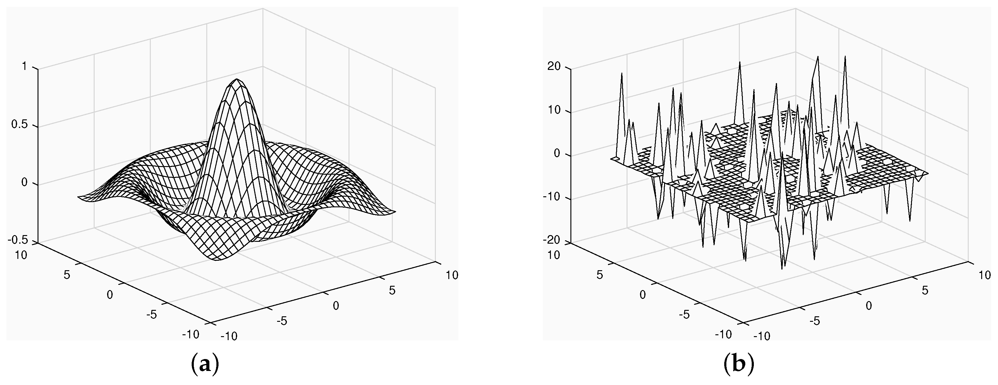
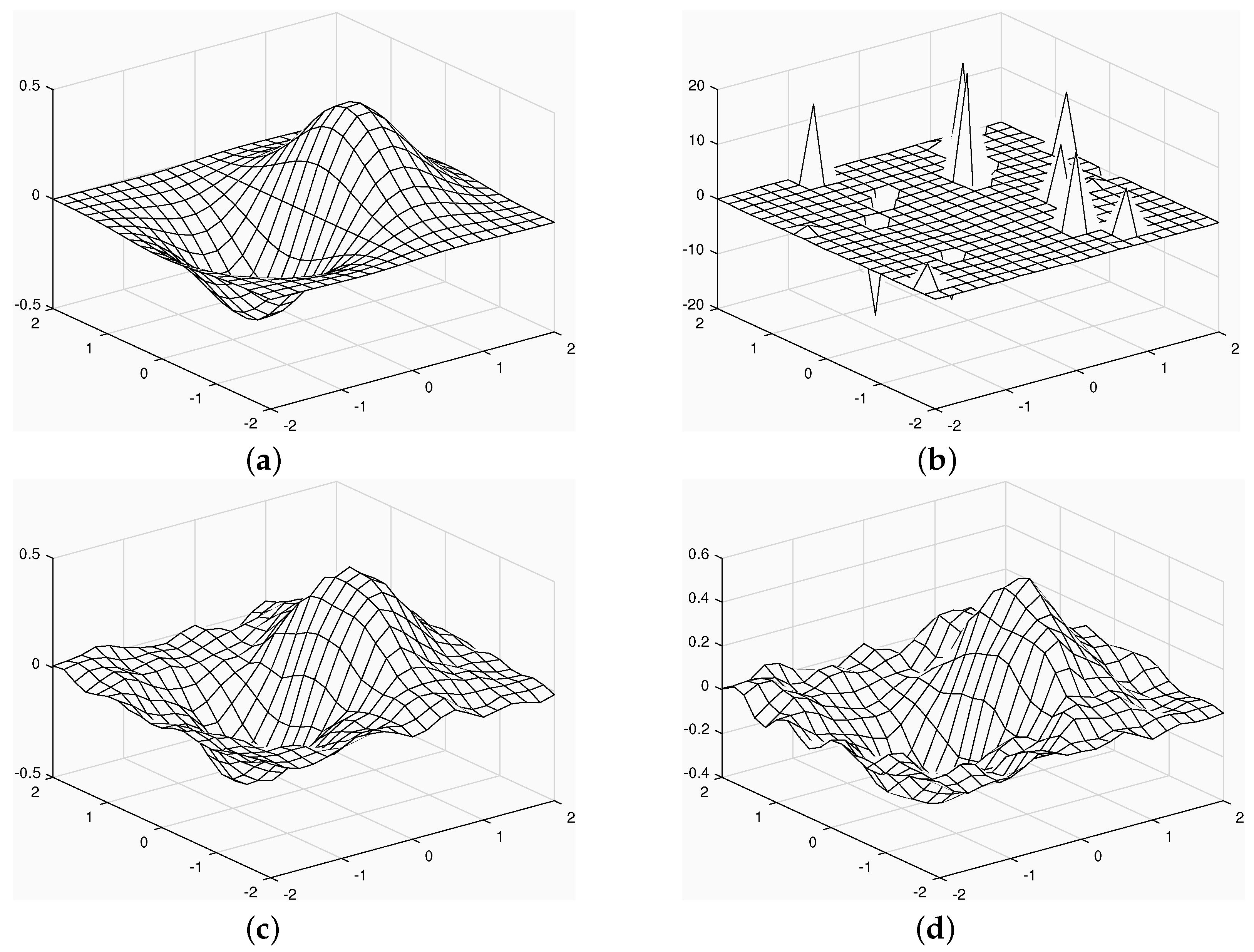
Example 1.

The binary continuous function f is a given as follows:

$$\begin{array}{c}\hfill f(x,y)=50sinc\left(\pi \sqrt{x^2+y^2}\right),\end{array}$$

(41)

where$x\in [-1,1]$, $y\in [-1,1]$(two dimensions, respectively, take 21 discrete points),$sinc\left(x\right)=\frac{sin\left(\pi x\right)}{\pi x}$. After discretization of f, 20 dB Gaussian noise and 10% outlier noise were added to obtain the final degraded data.

In order to show the experimenta results of different examples, we will show the ground-truth data, the degraded data polluted by noise and outliers, and the restored outcome calculated by the proposed method and the KROMP method, respectively.

Example 2.

The binary continuous function f is a given as follows:

$$\begin{array}{c}\hfill f(x,y)=\frac{sin\sqrt{x^2+y^2}}{\sqrt{x^2+y^2}},\end{array}$$

(42)

where$x\in [-8,8]$,$y\in [-8,8]$(two dimensions, respectively, take 31 discrete points),$sinc\left(x\right)=\frac{sin\left(\pi x\right)}{\pi x}$. After discretization of f which is a binary continuous function, 10 dB Gaussian noise and 10% outlier noise were added to obtain the final degraded data.

From Figure 1 and Figure 2, although the shape of ground-truth in Example 2 is similar to that of Example 1 (see Figure 1a and Figure 2a), in fact, the degree of degradation of Example 2 is much greater than that of Example 1, which the function value and the degree of noise pollution are different (see Figure 1b and Figure 2b). The proposed method has obvious restorated outcomes, and can effectively recover original data (see Figure 1c, however the restorated outcomes of the KROMP method still have obvious noise residual in Figure 1d and Figure 2d. It also shows the effectiveness of the proposed method.

Figure 1. In Example 1, the ground-truth $\mathbf{f}$ was degraded by 20 dB Gaussian noise and 10% outliers, and the visual results of restoration by each method were obtained. (a) Ground-truth; (b) degraded; (c) the restored outcome by the proposed method, (d) the restored outcome by the KROMP method.

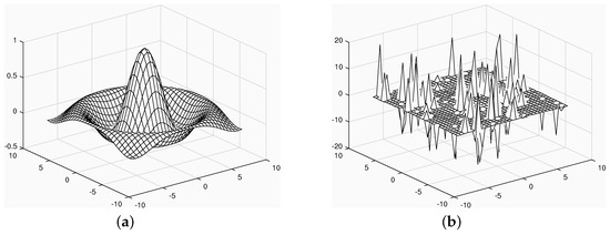
Figure 2. In Example 2, the real data $\mathbf{f}$ was degraded by 10 dB Gaussian noise and 10% outliers, and the visual results of restoration by each method were obtained. (a) Ground-truth; (b) degraded; (c) the restored outcome by the proposed method, (d) the restored outcome by the KROMP method.

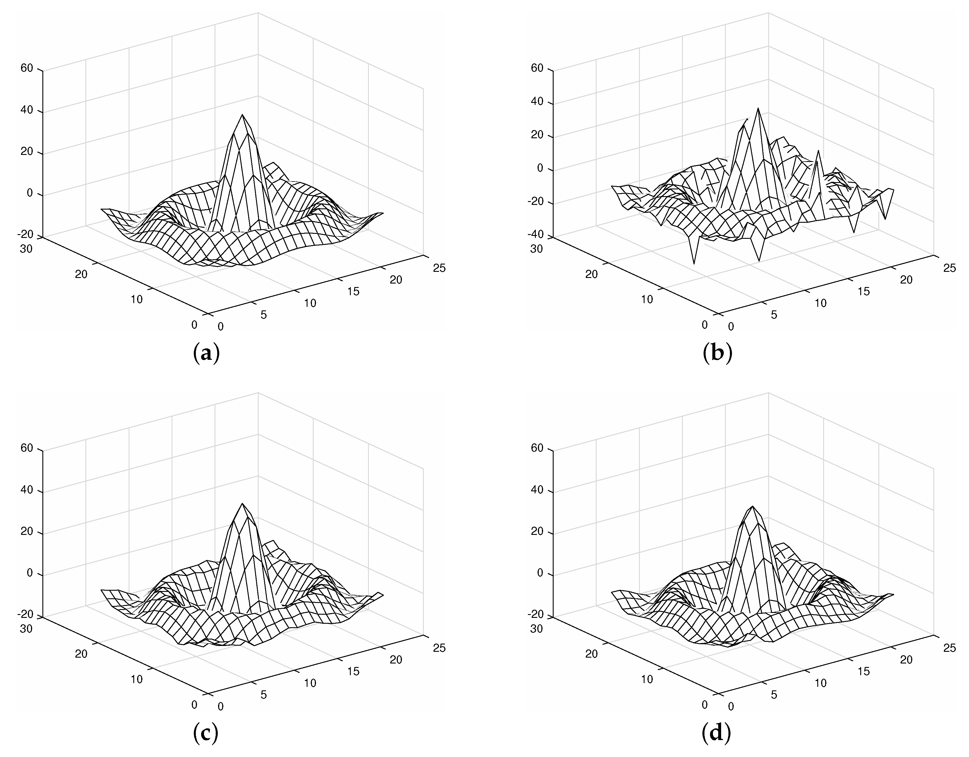
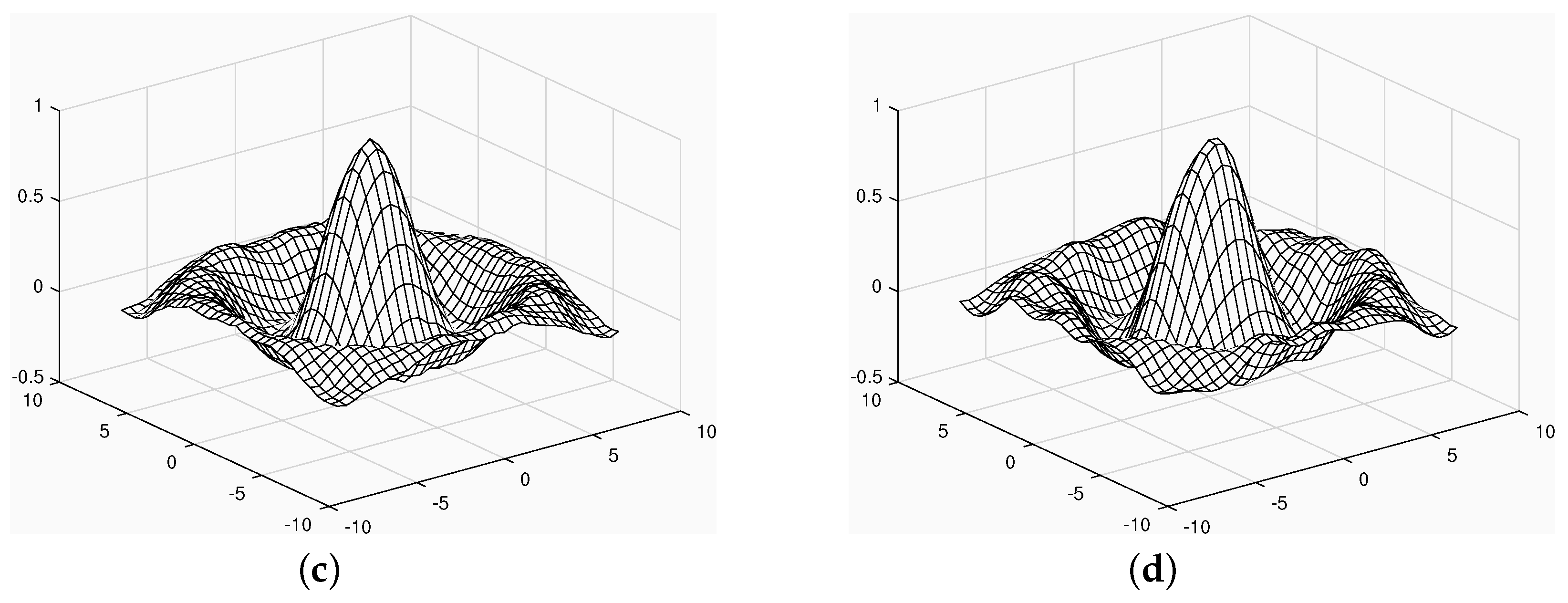
Example 3.

The binary continuous function f is a given as follows

$$\begin{array}{c}\hfill f(x,y)=xexp\left(-x^2-y^2\right),\end{array}$$

(43)

where$x\in [-2,2]$,$y\in [-2,2]$(two dimensions, respectively, take 21 discrete points). After discretization of f which is a binary continuous function, 10 dB Gaussian noise and 5% outlier noise were added to obtain the final degraded data.

It can be seen that even in the case of extremely large external pollution, such as Example 3 in Figure 3b, the proposed method can obtain more accurate recovery data (Figure 3c) than the KROMP method (Figure 3d). In addition, the relative error (ReErr) results from Example 1 to Example 3 are shown in Table 1, and the better results have been bolded. It is obvious that the proposed method has smaller relative errors compared with the KROMP method, which verifies the effectiveness of the proposed method.

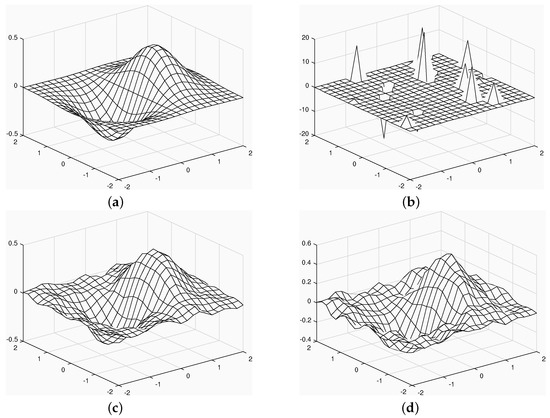
Figure 3. In Example 3, the real data $\mathbf{f}$ was degraded by 10 dB Gaussian noise and 5% outliers, and the visual results of restoration by each method were obtained. (a) Ground-truth; (b) degraded; (c) the restored outcome by the proposed method, (d) the restored outcome by the KROMP method.

Table 1. The ReErr results from Example 1 to Example 3 (Bold: the best).

	KROMP	Proposed
Example 1	0.128	0.116
Example 2	0.257	0.159
Example 3	0.178	0.117

5. Conclusions

In this paper, we proposed a new nonconvex modeling to deal with a challenging symmetry ill-posed problem. An efficient algorithm for solving the given nonconvex problem is designed by MPEC and the proximal-based regularization. Theoretically, the bounded sequence generated by the designed algorithm can be guaranteed to converge to the nonconvex problem’s local optimal solution. Furthermore, the convergence of the designed algorithm can be guaranteed for any initial value. The numerical experiments show that the proposed method can achieve better restoration results. For example, our method could obtain smaller relative error comparing with benchmark KROMP approach, besides, could interpolate more mesh points and significantly reduce noise.

References

- Tanaka, K. Generation of point sets by convex optimization for interpolation in reproducing kernel Hilbert spaces. Numer. Algorithms 2020, 84, 1049–1079. [Google Scholar] [CrossRef] [Green Version]
- Mo, Y.; Qian, T.; Mai, W.X.; Chen, Q.H. The AFD methods to compute Hilbert transform. Appl. Math. Lett. 2015, 45, 18–24. [Google Scholar] [CrossRef]
- Karvonen, T.; Särkkä, S.; Tanaka, K. Kernel-based interpolation at approximate Fekete points. Numer. Algorithms 2020, 84, 1049–1079. [Google Scholar]
- Silalahi, D.D.; Midi, H.; Arasan, J.; Mustafa, M.S.; Caliman, J.P. Kernel Partial Least Square Regression with High Resistance to Multiple Outliers and Bad Leverage Points on Near-Infrared Spectral Data Analysis. Symmetry 2021, 13, 547. [Google Scholar] [CrossRef]
- Deng, L.J.; Guo, W.H.; Huang, T.Z. Single-image super-resolution via an iterative reproducing kernel Hilbert space method. IEEE Trans. Circuits Syst. Video Technol. 2015, 26, 2001–2014. [Google Scholar] [CrossRef]
- Li, X.Y.; Wu, B.Y. A new reproducing kernel collocation method for nonlocal fractional boundary value problems with non-smooth solutions. Appl. Math. Lett. 2018, 86, 194–199. [Google Scholar] [CrossRef]
- Wu, Q.; Li, Y.; Xue, W. A Kernel Recursive Maximum Versoria-Like Criterion Algorithm for Nonlinear Channel Equalization. Symmetry 2019, 11, 1067. [Google Scholar] [CrossRef] [Green Version]
- Papageorgiou, G.; Bouboulis, P.; Theodoridis, S. Robust kernel-based regression using orthogonal matching pursuit. In Proceedings of the IEEE International Workshop on Machine Learning for Signal Processing, Southampton, UK, 22–25 September 2013; pp. 1–6. [Google Scholar]
- Chen, S.S.; Donoho, D.L.; Saunders, M.A. Atomic decomposition by basis pursuit. SIAM Rev. 2001, 43, 129–159. [Google Scholar] [CrossRef] [Green Version]
- Donoho, D.L. For most large underdetermined systems of linear equations the minimial ℓ1-norm solution is also the sparsest solution. Commun. Pure Appl. Math. 2006, 59, 797–829. [Google Scholar] [CrossRef]
- Dong, B.; Zhang, Y. An efficient algorithm for ℓ0 minimization in wavelet frame based image restoration. J. Sci. Comput. 2013, 54, 350–368. [Google Scholar] [CrossRef] [Green Version]
- Zuo, W.M.; Meng, D.Y.; Zhang, L.; Feng, X.C.; Zhang, D. A generalized iterated shrinkage algorithm for non-convex sparse coding. In Proceedings of the IEEE International Conference on Computer Vision, Sydney, Australia, 1–8 December 2013; pp. 217–224. [Google Scholar]
- Ye, J.J.; Zhu, D. New necessary optimality conditions for bilevel programs by combining the MPEC and value function approaches. SIAM J. Optim. 2010, 20, 1885–1905. [Google Scholar] [CrossRef]
- Yuan, G.Z.; Ghanem, B. ℓ0 TV: A sparse optimization method for impulse noise image restoration. IEEE Trans. Pattern Anal. Mach. Intell. 2017, 41, 352–364. [Google Scholar] [CrossRef] [Green Version]
- Yuan, G.Z.; Ghanem, B. An exact penalty method for binary optimization based on MPEC formulation. In Proceedings of the AAAI Conference on Artificial Intelligence, San Francisco, CA, USA, 4–9 February 2017. [Google Scholar]
- Attouch, H.; Bolte, J.; Redont, P. and Soubeyran, A. Proximal alternating minimization and projection methods for nonconvex problems. An approach based on the Kurdyka–Lojasiewicz inequality. Math. Oper. Res. 2010, 35, 435–457. [Google Scholar] [CrossRef] [Green Version]
- Wang, Y.J.; Dong, M.M.; Xu, Y. A sparse rank-1 approximation algorithm for high-order tensors. Appl. Math. Lett. 2020, 102, 106–140. [Google Scholar] [CrossRef]
- Bolte, J.; Sabach, S.; Teboulle, M. Proximal alternating linearized minimization or nonconvex and nonsmooth problems. Math. Program. 2014, 146, 459–494. [Google Scholar] [CrossRef]
- Sun, T.; Barrio, R.; Jiang, H.; Cheng, L.Z. Convergence rates of accelerated proximal gradient algorithms under independent noise. Numer. Algorithms 2019, 81, 631–654. [Google Scholar] [CrossRef]
- Hu, W.; Zheng, W.; Yu, G. A Unified Proximity Algorithm with Adaptive Penalty for Nuclear Norm Minimization. Symmetry 2019, 11, 1277. [Google Scholar] [CrossRef] [Green Version]
- An, Y.; Zhang, Y.; Guo, H.; Wang, J. Compressive Sensing Based Three-Dimensional Imaging Method with Electro-Optic Modulation for Nonscanning Laser Radar. Symmetry 2020, 12, 748. [Google Scholar] [CrossRef]
- Ma, F. Convergence study on the proximal alternating direction method with larger step size. Numer. Algorithms 2020, 85, 399–425. [Google Scholar] [CrossRef]
- Pham, Q.M.; Lachmund, D.; Hào, D.N. Convergence of proximal algorithms with stepsize controls for non-linear inverse problems and application to sparse non-negative matrix factorization. Numer. Algorithms 2020, 85, 1255–1279. [Google Scholar] [CrossRef]
- Tiddeman, B.; Ghahremani, M. Principal Component Wavelet Networks for Solving Linear Inverse Problems. Symmetry 2021, 13, 1083. [Google Scholar] [CrossRef]
- Xu, Y.Y.; Yin, W.T. A block coordinate descent method for regularized multiconvex optimization with applications to nonnegative tensor factorization and completion. SIAM J. Imaging Sci. 2013, 6, 1758–1789. [Google Scholar] [CrossRef]
Publisher’s Note: MDPI stays neutral with regard to jurisdictional claims in published maps and institutional affiliations. |
© 2021 by the authors. Licensee MDPI, Basel, Switzerland. This article is an open access article distributed under the terms and conditions of the Creative Commons Attribution (CC BY) license (https://creativecommons.org/licenses/by/4.0/).