The Bipartite and Tripartite Entanglement in $\mathcal{PT}$-Symmetric System

Abstract

We consider a $\mathcal{PT}$-symmetric system that involves three optical resonant elements coupled together. We investigate the quantum correlations between subsystems by calculating bipartite and tripartite entanglement. We show that when $\mathcal{PT}$-symmetry is maintained, the correlations between subsystems strongly depend on the parameters describing the interaction between them and characterizing the gain and loss of energy in the system’s active and passive elements. We estimate the range of interaction parameter values for which the strongest bipartite and tripartite entanglement can be produced. Additionally, we show that the discussed system can be a source of stable entangled states.

1. Introduction

For a long time, one of the most crucial rules of quantum mechanics was the assumption that the Hamiltonian related to the given quantum system must be Hermitian. The reason for such limitation was simple: all eigenvalues of the Hamiltonian must be real. Because of that, many of the physical systems described by the non-Hermitian Hamiltonian were ignored. However, in 1998 Bender and Boettcher showed that there exists a spectrum of non-Hermitian Hamiltonians, which still possesses real and positive eigenvalues [1]. Such systems have been reviewed with hundreds of papers published, dozens of conferences held, and many dissertations conducted, opening new development directions for quantum mechanics. The key idea here is to provide conditions for maintaining so-called $\mathcal{PT}$-symmetry instead of Hermiticity. Once the $\mathcal{PT}$-symmetry is not broken, the Hamiltonian still exhibits properties that are satisfactory to describe a quantum system in the same way as it would have been done by a Hermitian Hamiltonian. The emergence of $\mathcal{PT}$-symmetrical Hamiltonians is not in conflict with quantum mechanics that developed over many decades. Instead, it is rather an alternative to Hermitian operators that allows us to study new quantum theories that may describe measurable physical phenomena. The appearance of the $\mathcal{PT}$-symmetry was initially seen as a mathematically interesting finding, and the first analyzed $\mathcal{PT}$-symmetric Hamiltonian was $\widehat{H}={\widehat{p}}^2+i{\widehat{x}}^3$ [1,2,3].

When considering the $\mathcal{PT}$-symmetric system, one can witness a phase-transition point at which the system loses its $\mathcal{PT}$-symmetric properties. In other words, a given system may be in the $\mathcal{PT}$-symmetric phase, where all eigenvalues of the Hamiltonian are real, or in $\mathcal{PT}$-symmetry broken phase, where we have complex eigenvalue spectra. The transition point from one phase to the other is called an exceptional point [4] and it is usually connected with one of the system parameters. It should be noted that the $\mathcal{PT}$-symmetry breaking point does not have to be manifested physically, but the overall change of that parameter itself may significantly change the physical state [5].

Over the last years, different kinds of $\mathcal{PT}$-symmetric systems have been considered. In the field of materials research, it was found that at the vicinity of the symmetrical breakout point, some materials with $\mathcal{PT}$-symmetry structure behave as unidirectional invisible media [3]. Some other materials show unidirectional reflectionless near spontaneous parity-time symmetry phase transition point [6]. In the field of optical waveguides, it has been found that in specially designed pseudo-Hermitian potentials, the phase transition point can create a loss-induced optical transparency [7]. In the laser study, the unique property of the $\mathcal{PT}$-symmetric system also leads to the loss-induced suppression and revival of lasing at the phase transition points [8], making the effectiveness of the single-mode operation in microring laser resonators [9]. Moreover, one can use $\mathcal{PT}$-symmetric systems to study dissipative quantum systems [10] as well as to learn about signal generation and processing based on the properties of $\mathcal{PT}$-symmetric systems in microwave photonics [11]. In the same $\mathcal{PT}$-symmetrical systems, the asymmetric transmission of photons in an optical dimer has been studied in addition to the nonlinear properties that influence the propagation of optical pulses [12,13,14,15]. Additionally, $\mathcal{PT}$-symmetric systems can be also used to unveil the nonlocal particle current localized at the edges due to the interplay between $\mathcal{PT}$-symmetry and topology [16] at both direct and bidirectional phase transitions [17] in the field of superconductivity. Further, in the field of quantum information, $\mathcal{PT}$-symmetry could create new methods to control light such as transport control of a confined single-photon [18,19,20] is intended to use light beams to transmit information in quantum computers to replace conventional electrical wires in conventional computers. It will be a large step forward for the realization of the quantum internet in the future. To accomplish that, the study of quantum correlation between subsystems in a $\mathcal{PT}$-symmetric system is very significant and plays a fundamental role, especially the balance of gain and loss for $\mathcal{PT}$-symmetry in the quantum system and the unique properties when $\mathcal{PT}$-symmetry breaking occurs [21,22,23].

In our paper, we consider the $\mathcal{PT}$-symmetric system consisting of the three interacting cavities and study the possibility of entanglement appearance. The ability to create a highly entangled quantum state plays a significant role in quantum information theory. States that carry such a valuable resource have a vast amount of applications. Quantum teleportation, quantum cryptography, and quantum computation are primarily based on quantum entanglement. In general, quantum correlations are an indispensable part of quantum information theory. For this reason, it is necessary to explore and understand the entanglement in quantum systems. Although in recent years there were a lot of quality results concerning entanglement in bipartite systems, the quantum correlations in more complex systems consisting of two or higher number of subsystems require further analysis and answers. This fact is a good motivation to search systems that can be the source of entangled states.

This paper is organized as follows. In Section 2, we describe the $\mathcal{PT}$-symmetric system of three coupled optical resonant elements. The first and last subsystems are passive and active, respectively, which corresponds to the loss and gain of energy. In Section 3, we investigate the entanglement in the $\mathcal{PT}$-symmetric phase. We examine the quantum correlations between two of the three resonant elements and also consider the correlations between the three subsystems by determining the bipartite and tripartite entanglement. Finally, our conclusions are drawn in Section 4. One should note that our work strongly refers to another paper concerning PT -symmetrical system, namely [24], and should be considered more as a follow-up. Although here we are considering only three cavities, we approach the bipartite negativity more thoroughly. Additionally, we present the results for tripartite negativity and steady-state solutions.

2. The Model

Our model consists of three cavities that belong to a chain. The first cavity (labeled by 1) is passive, and the last one (labeled by 3) is active, which means they correspond to the loss and gain of energy, respectively. These cavities are not coupled directly, but they are simultaneously coupled to the middle one (labeled by 2) that is not with loss or gain—see Figure 1. This system can be described by the Hamiltonian:

$$\begin{array}{ccc}\hfill \widehat{H}& =& \left(\omega -i\gamma \right){\widehat{a}}_1^{†}{\widehat{a}}_1+\omega {\widehat{a}}_2^{†}{\widehat{a}}_2+\left(\omega +i\gamma \right){\widehat{a}}_3^{†}{\widehat{a}}_3+\beta \left({\widehat{a}}_1^{†}{\widehat{a}}_2+{\widehat{a}}_2^{†}{\widehat{a}}_1+{\widehat{a}}_2^{†}{\widehat{a}}_3+{\widehat{a}}_3^{†}{\widehat{a}}_2\right)\hfill \\ & =& \left(\begin{array}{ccc}{\widehat{a}}_1^{†}& {\widehat{a}}_2^{†}& {\widehat{a}}_3^{†}\end{array}\right){\widehat{H}}_0\left(\begin{array}{c}{\widehat{a}}_1\\ {\widehat{a}}_2\\ {\widehat{a}}_3\end{array}\right)=\left(\begin{array}{ccc}{\widehat{a}}_1^{†}& {\widehat{a}}_2^{†}& {\widehat{a}}_3^{†}\end{array}\right)\left(\begin{array}{ccc}\omega -i\gamma & \beta & 0\\ \beta & \omega & \beta \\ 0& \beta & \omega +i\gamma \end{array}\right)\left(\begin{array}{c}{\widehat{a}}_1\\ {\widehat{a}}_2\\ {\widehat{a}}_3\end{array}\right),\hfill \end{array}$$

(1)

where ${\widehat{a}}_n^{†}$ and ${\widehat{a}}_n$ (n = 1,2,3) are the creation and annihilation operators for the i-th cavity. The parameter $\omega$ is the resonant frequency characterizing cavities, while the parameter $\beta$ describes the linear interaction between the two subsystems. In our model, we set the cavities to have the same resonant frequency, and we assume the same strength of the interactions between them. Moreover, the rates of loss and gain of energy in cavities 1 and 3 are assumed to be the same and equal to $\gamma$.

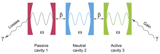
Figure 1. Scheme of the model.

One can easily show that the Hamiltonian ${\widehat{H}}_0$ is not Hermitian but fulfills both $\mathcal{P}$ symmetry (partial reflection 1 ⟷ 3) and $\mathcal{T}$ symmetry (time inverse i ⟷ - i) [25]. Because the Hamiltonian ${\widehat{H}}_0$ is $\mathcal{PT}$-symmetric, the phase transition of the system occurs. At this point, the system goes from an unbroken $\mathcal{PT}$-symmetry phase to a broken $\mathcal{PT}$-symmetry phase. This point is called an exceptional point and for our system is placed at $\gamma =\sqrt{2}\beta$ (for more details, see [25]). If the parameters $\beta$ and $\gamma$ obey the relation $\gamma <\sqrt{2}\beta$, then all eigenvalues of Hamiltonian are real, and the system is in the unbroken $\mathcal{PT}$-symmetry phase. In the other case, when $\gamma >\sqrt{2}\beta$, complex eigenvalues appear, and the system is in the broken $\mathcal{PT}$-symmetry phase.

As our system exchanges energy with the environment, to analyze its evolution, we need to use the master equation. The time evolution of density matrix $\widehat{\rho }$ is determined by

$$\frac{d}{dt}\widehat{\rho }=-i\left[{\widehat{H}}_I,\widehat{\rho }\right]+\mathcal{L}\widehat{\rho },$$

(2)

where ${\widehat{H}}_I$ is the Hermitian part of Hamiltonian $\widehat{H}$

$${\widehat{H}}_I=\omega \left({\widehat{a}}_1^{†}{\widehat{a}}_1+{\widehat{a}}_2^{†}{\widehat{a}}_2+{\widehat{a}}_3^{†}{\widehat{a}}_3\right)+\beta \left({\widehat{a}}_1^{†}{\widehat{a}}_2+{\widehat{a}}_2^{†}{\widehat{a}}_1+{\widehat{a}}_2^{†}{\widehat{a}}_3+{\widehat{a}}_3^{†}{\widehat{a}}_2\right),$$

(3)

and $\mathcal{L}$ is the Liouvillian superoperator:

$$\mathcal{L}\widehat{\rho }=\gamma \left(2{\widehat{a}}_1\widehat{\rho }{\widehat{a}}_1^{†}-{\widehat{a}}_1^{†}{\widehat{a}}_1\widehat{\rho }-\widehat{\rho }{\widehat{a}}_1^{†}{\widehat{a}}_1\right)+\gamma \left(2{\widehat{a}}_3^{†}\widehat{\rho }{\widehat{a}}_3-{\widehat{a}}_3{\widehat{a}}_3^{†}\widehat{\rho }-\widehat{\rho }{\widehat{a}}_3{\widehat{a}}_3^{†}\right).$$

(4)

In our analysis, we assume that only one of the three cavities is initially in the one-photon state $|1⟩$, while the other two are in vacuum state $|0⟩$. In other words, we consider three initial scenarios:

• $\widehat{\rho }(t=0)=|100⟩⟨100|$;
• $\widehat{\rho }(t=0)=|010⟩⟨010|$;
• $\widehat{\rho }(t=0)=|001⟩⟨001|$,

where $|ijk⟩={|i⟩}_1\otimes {|j⟩}_2\otimes {|k⟩}_3$ are three-mode states. The first state represents a scenario where only the passive cavity is initially in a one-photon state and the density matrix $\widehat{\rho }(t=0)=|100⟩⟨100|$. The next state corresponds to a scenario when the middle cavity (neutral) is in a one-photon state which is represented by the density matrix $\widehat{\rho }(t=0)=|010⟩⟨010|$. In the last case, we consider the situation when the system starts its evolution from the state $\widehat{\rho }(t=0)=|001⟩⟨001|$ and only the active cavity is in the one-photon state.

3. The Entanglement

Let us now investigate the entanglement generation in a $\mathcal{PT}$-symmetric three-mode system. We will analyze the bipartite entanglement between cavities $1-2$, $2-3$, and $1-3$. Additionally, we will study the tripartite entanglement between all three cavities. It should be cleared out that through all numerical analysis we assumed that the dimensionality of our tripartite system was equal to $10\otimes 10\otimes 10$. Such a dimension was large enough to analyze the dynamics of the system, and further increasing the system’s dimension did not change the obtained values of negativities. On the other hand, it was so low that numerical calculations could be performed quickly.

To quantify the two-mode entanglement, we will use an entanglement measure called negativity, which is based on the partial transposition criterion [26,27]. The bipartite negativity of two-mode state ${\rho }_{ij}$ is defined as

$$N_{ij}=N\left({\rho }_{ij}\right)=-2\sum _n{\lambda }_n({\rho }_{ij}^{T_i})$$

(5)

where ${\rho }_{ij}^{T_i}$ describes the partial transposition (with respect to i mode) of the reduced density matrix ${\rho }_{ij}=T{r}_k\left({\rho }_{ijk}\right)$ and ${\lambda }_n$ are the negative eigenvalues calculated for ${\rho }_{ij}^{T_i}$. The negativity of the separable state takes 0 and reaches its maximal value for the maximally entangled state.

The results of our analysis are illustrated in Figure 2, where we present the time evolution of negativity for three initial states and two values of $\gamma /\beta$, namely $\gamma /\beta \in \{0.01,0.8\}$.

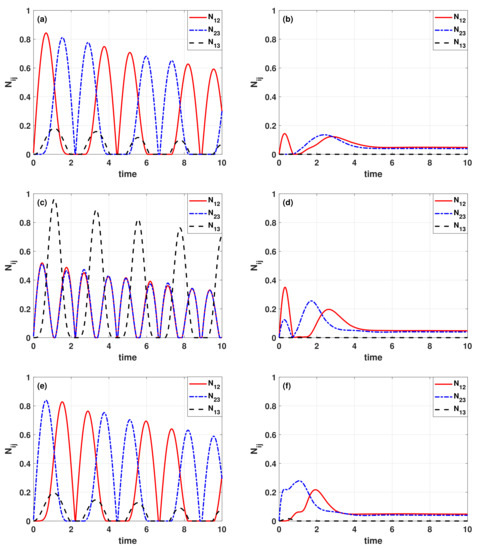
Figure 2. The time evolution of bipartite negativities $N_{ij}$: (a) $\widehat{\rho }(t=0)=|100⟩⟨100|$, $\gamma =0.01\beta$; (b) $\widehat{\rho }(t=0)=|100⟩⟨100|$, $\gamma =0.8\beta$; (c) $\widehat{\rho }(t=0)=|010⟩⟨010|$, $\gamma =0.01\beta$; (d) $\widehat{\rho }(t=0)=|010⟩⟨010|$, $\gamma =0.8\beta$; (e) $\widehat{\rho }(t=0)=|001⟩⟨001|$, $\gamma =0.01\beta$; (f) $\widehat{\rho }(t=0)=|001⟩⟨001|$, $\gamma =0.8\beta$.

In the beginning, we analyze the situation when our system is initially in the state $\widehat{\rho }(t=0)=|100⟩⟨100|$, where only the passive cavity is excited. In the Figure 2a, we can observe the time evolution of negativities $N_{12},N_{13},\mathrm{and}{N}_{23}$ for $\gamma /\beta =0.01$. The change of negativities is periodical. The oscillation periods of the negativities $N_{12}$ and $N_{23}$ are equal and shifted in time. Thus, we conclude that the generation of entanglements characterized by $N_{12}$ and $N_{23}$ is strongly correlated with each other. The maximum value of the negativity for subsystems 1 and 2 is greater than 0.84, while for a pair of subsystems $2-3$ is only slightly smaller. On the other hand, the entanglement between subsystems $1-3$ is significantly weaker and reaches its maximum value when the negativities $N_{12}$ and $N_{23}$ have the same value. This situation completely changes when we set $\gamma /\beta =0.8$ (see Figure 2b). Now the maximum values of negativities are smaller than in the previous case for all subsystem pairs. What is interesting is, the entanglement between cavities 1 and 3 is no longer produced. This situation is caused by a stronger interaction with the environment. At the beginning of the system’s evolution, we can detect entanglement only between subsystems 1 and 2. Then, as the system evolves, the entanglement between subsystems 2 and 3 appears. After a certain point, the evolution of negativities stabilizes around some value.

In the next analyzed case with the initial state $\widehat{\rho }(t=0)=|010⟩⟨010|$, only the second subsystem (neutral cavity) is excited. As previously, we consider two sub-cases for two various values of $\gamma /\beta$ (see Figure 2c,d). When $\gamma =0.01\beta$, the bipartite entanglements between the subsystems also change periodically, and the amplitude of oscillations decreases in time. The oscillation period of the negativities $N_{12}$ and $N_{23}$ takes the same value. However, the evolutions of negativities $N_{12}$ and $N_{23}$ are approximately the same, so they are not shifted in time. Moreover, the maximum values of $N_{12}$ and $N_{23}$ are smaller (mostly below 0.5) than in the situation when only the passive cavity is initially excited. Interestingly, the maximum value of negativity $N_{13}$ is slightly higher than $0.95$ and periodically dominates the values $N_{12}$ and $N_{23}$. This situation is opposite to the first initial scenario. Specifically, when $N_{13}$ reaches its maximal value, the negativities $N_{12}$ and $N_{23}$ are equal to zero simultaneously. When we increase the value of the gain/loss parameter in the unbroken $\mathcal{PT}$-symmetry phase (see Figure 2d), the entanglement between subsystems 1 and 3 is no longer produced like in the first case. Thus one can conclude that for a specific rate $\gamma /\beta =0.8$, the interaction with the environment plays the most significant role. We see that negativities $N_{12}$ and $N_{23}$ initially oscillate. These oscillations disappear after a time, and $N_{12}$ together with $N_{23}$ converge to fixed, equal values. These values are the same as in the first scenario, with $\gamma /\beta =0.8$.

In the third scenario, the system’s evolution starts from the state $\widehat{\rho }(t=0)=|001⟩⟨001|$. It means that only the third cavity (active cavity) is initially excited. As previously, we concentrate on two cases, $\gamma =0.01\beta$ and $\gamma =0.8\beta$. The results of our calculations are illustrated in Figure 2e,f. We see that when $\gamma =0.01\beta$, the evolutions of the negativities seems to be similar to the case where only the passive cavity is initially excited (see Figure 2a). It means the negativities $N_{12}$ and $N_{23}$ oscillate and can be characterized by the same period of changes. Here, the negativity $N_{13}$ also reaches its maximum value when $N_{12}=N_{23}$. The maximum value of $N_{13}$ is dominated by the maximum values of $N_{12}$ and $N_{23}$. The entanglement between subsystems 1 and 3 is weaker than the entanglement between other subsystem pairs. When we compare the results presented in Figure 2a,e, we see that there is an inversion between the evolutions of $N_{12}$ and $N_{23}$, while $N_{13}$ evolves in the same way. When initially the active cavity is excited, $N_{23}$ reaches its maximum value earlier than $N_{12}$. It is contrary to the situation of the initial state of the system is $\widehat{\rho }(t=0)=|100⟩⟨100|$. For higher values of $\gamma /\beta$ (see Figure 2f), we can also notice inversion in the generation of entanglements compared to the situation shown in Figure 2b. At the beginning of the system’s evolution, we see the entanglement between subsystems 2 and 3 appears first. After that, a very weak entanglement between cavities 1 and 3 is generated. At last, the entanglement between subsystems 1 and 2 appears. This entanglement is slightly weaker than between subsystems 2 and 3. What is interesting, contrary to the situation depicted in Figure 2b, we can observe the entanglement between subsystems 1 and 3. As in the first and second scenario, the evolution of negativities stabilizes around the same value.

From the above discussion, we can conclude that the maximal degree of bipartite entanglement strongly depends on the value of the parameter $\gamma$. This dependence is better visible in Figure 3, where we show the relation between the maximal values of negativity and ratio $\gamma /\beta$. Figure 3a–c correspond to three various initial states. Now let us investigate maximal values of entanglement in the context of ratio $\gamma /\beta$.

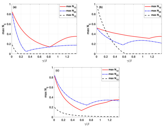
Figure 3. Maximal values of the bipartite negativities $N_{ij}$ versus $\gamma /\beta$ for $\omega =5\beta$ and for various initial states $\widehat{\rho }(t=0)$: (a) $|100⟩⟨100|$, (b) $|010⟩⟨010|$, (c) $|001⟩⟨001|$.

We started by considering the situation when the first cavity (passive cavity) is excited, which corresponds to the initial state $\widehat{\rho }(t=0)=|100⟩⟨100|$. As Figure 3a shows, only the entanglement between modes 1−2 and 2−3 can be produced for all considered values of the ratio $\gamma /\beta$. Whereas the entanglement between subsystems 1 and 3 is only generated for small values of the $\gamma /\beta$ parameter. What is relevant is, the amount of entanglement appearing in the system strongly depends on the value of the gain/loss parameter. In the beginning, the maximal values of $N_{12}$ and $N_{23}$ both initially decrease, and then they start to increase. This change of monotonicity can be observed for $N_{12}$ at $\gamma /\beta \approx 0.82$ and $N_{23}$ from $\gamma /\beta \approx 0.31$. It should be noted that for all values of $\gamma /\beta$, the entanglement between cavities 1 and 2 is stronger than other bipartite entanglements. For the $\gamma /\beta$ values that are close to the exceptional point, the maximal negativities are $N_{12}\approx 0.35$ and $N_{23}\approx 0.18$. The weakest entanglement is produced between the first and third cavities. In such a case, the negativity $N_{13}$ decreases from a small value $N_{13}\approx =0.2$ and disappears from $\gamma /\beta =0.18$.

In the case of the initial state $\widehat{\rho }(t=0)=|010⟩⟨010|$ (see Figure 3b), the bipartite entanglements between subsystems pairs 1−2 and 2−3 are weaker than this between subsystems 1 and 3 for some initial range of parameter $\gamma /\beta$. It is contrary to the previous case. While the value of ratio $\gamma /\beta$ increases, the maximal value of $N_{13}$ decreases from approx $0.96$ and starts to reach a value close to zero for $\gamma /\beta \approx 0.65$. The maximal values of $N_{12}$ and $N_{23}$ are approximately equal to $0.5$ for $\gamma /\beta =0$. When we increase the ratio $\gamma /\beta$, the entanglements between subsystem pairs 1−2 and 2−3 decrease, but these drops are slower than those observed in the case of $\widehat{\rho }(t=0)=|100⟩⟨100|$. Additionally, the maximal values of $N_{12}$ are always higher than those obtained for $N_{23}$.

In the last case, the system’s evolution starts from the state $\widehat{\rho }(t=0)=|001⟩⟨001|$, and the excitation initially appears in the active cavity. In the Figure 3c, we see that analogously to the first case, the weakest entanglement appears between subsystem pairs 1−3. However, this time it decreases slower with changing parameter $\gamma /\beta$ and reaches almost zero at the exceptional point. This drop is slower than in the two previous cases. Moreover, the entanglement between subsystems 2 and 3 for $\gamma \le 1.27\beta$ dominates almost for all range of considered values of $\gamma /\beta$. This trend continues until the ratio $\gamma /\beta$ reaches the exceptional point where again $N_{12}$ is greater than $N_{23}$.

In Figure 2, we see too that for time $t\to \infty$, all negativities describing the bipartite entanglement converge to a constant value. Therefore, in Figure 4, we present the negativities calculated for the system’s steady-state solution for various ratios $\gamma /\beta$. In the case of a steady-state solution, for very small values of $\gamma /\beta$, there are no bipartite entanglements generated. As the ratio $\gamma /\beta$ increases, the entanglements start slowly to appear. The entanglement 2−3 appears first, followed by the appearance of entanglement between 1−2. When the ratio $\gamma /\beta$ reaches $0.8$ and further increases towards the phase transition point, the entanglement between cavities 1 and 2 grows rapidly. At the same time, the negativity $N_{23}$ also increases but much slower than $N_{12}$. What is interesting, when the value of $\gamma /\beta$ is close to the phase transition point, stable entanglements are generated in our system. We do not observe entanglement between $1-3$ for steady-state solutions.

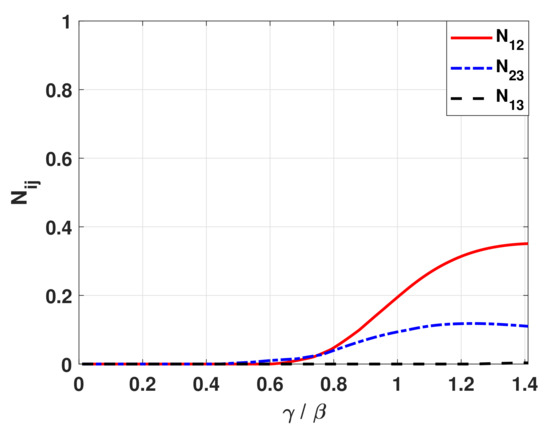
Figure 4. Steady-state solutions for bipartite negativities $N_{ij}$ versus the value of the ratio $\gamma /\beta$ for $\omega =5\beta$.

In further considerations, we discuss the generation of three-mode entanglement. For the analysis of the entanglement’s degree related to three cavities, we use the tripartite negativity. The tripartite negativity can be defined as [28]

$$N_{123}\left(\rho \right)=\sqrt[3]{N_{1-23}{N}_{2-13}{N}_{3-12}},$$

(6)

and the bipartite negativities can be written in the following form

$$N_{i-jk}=-2\sum _n{\sigma }_n\left({\rho }^{T_i}\right),$$

(7)

where ${\sigma }_n\left({\rho }^{T_i}\right)$ are the negative eigenvalues of ${\rho }^{T_i}$, which is the partial transpose of $\rho$ with respect to subsystem i, $⟨a_i,b_{jk}|{\rho }^{T_i}|c_i,d_{jk}⟩=⟨c_i,b_{jk}\left|\rho \right|a_i,d_{jk}⟩$, $i=1,2,3$, and $jk=23,13,12$. The negativities $N_{i-jk}$ describe the bipartite entanglements between subsystem i and the other two subsystems j and k which are considered as a whole.

In Figure 5, we present the time evolution of negativities related to three-mode entanglement for various initial states and different values of $\gamma /\beta$. Firstly, we consider the case when, at the beginning of the time evolution of the system, only the passive cavity is excited, while the other subsystems are in a vacuum state. We can see (in Figure 5a) that when $\gamma /\beta =0.01$, the time evolution of tripartite and all bipartite entanglements is oscillating with a small portion of damping. The oscillation periods of the negativities $N_{1-23}$ and $N_{3-12}$ are the same. Whereas the oscillation periods of $N_{123}$ and $N_{2-13}$ are twice as short as those of the other two negativities. There are situations when all bipartite entanglements ($N_{i-jk}$) disappear simultaneously. Consequently, the tripartite entanglement of the system also disappears at the same time. The bipartite negativity $N_{1-23}$ reaches the maximal value first. Then, almost simultaneously with $N_{1-23}$, $N_{2-13}$ achieves its maximal value. Subsequently, $N_{123}$ increases to the maximum, and finally, $N_{3-12}$ takes its maximal value as well. The negativity $N_{2-13}$ increases in the same way as $N_{1-23}$ and decreases in the same way with $N_{3-12}$. This relation is reversed after each period of its oscillation. The negativity $N_{2-13}$ increases and decreases in the same way as $N_{3-12}$ and $N_{1-23}$, respectively. When $\gamma =0.8\beta$, we can see that the bipartite entanglements between subsystems 1−23 and 2−13 appear firstly and simultaneously. Meanwhile, the other negativities are equal to zero (see Figure 5b). As the evolution continues, we can observe very weak entanglement between cavities 3−12, and thus, the tripartite negativity $N_{123}$ also takes nonzero values. Subsequently, we observe a rapid increase of all negativities. They reach their maximum values and then decrease gradually to constant values. We also see that among all bipartite entanglements, the entanglement between partitions 2−13 is the strongest, while the maximal strengths of entanglements 1−23 and 3−12 are lower and equal to each other. Moreover, when the tripartite entanglement is the strongest, the entanglement 2−13 is also the strongest, contrary to entanglements 1−23 and 3−12. Additionally, although the entanglement 3−12 appears last, it reaches its maximal value first. For a long-time limit when the values of all negativities stabilize, the entanglements 3−12 and 2−13 are the weakest and most powerful, respectively.

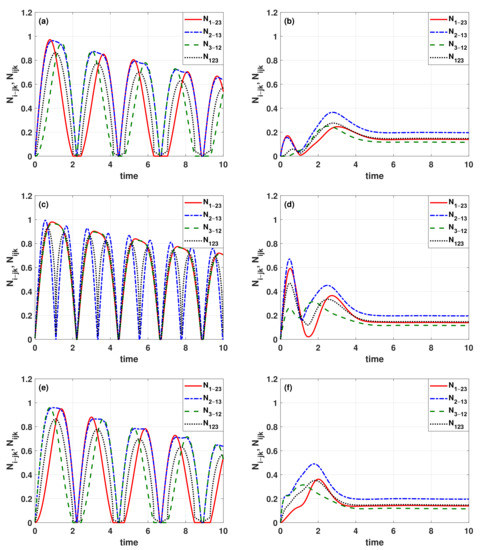
Figure 5. The time evolution of bipartite ($N_{i-jk}$) and tripartite ($N_{ijk}$) negativities: (a) $\widehat{\rho }(t=0)=|100⟩⟨100|$, $\gamma =0.01\beta$; (b) $\widehat{\rho }(t=0)=|100⟩⟨100|$, $\gamma =0.8\beta$; (c) $\widehat{\rho }(t=0)=|010⟩⟨010|$, $\gamma =0.01\beta$; (d) $\widehat{\rho }(t=0)=|010⟩⟨010|$, $\gamma =0.8\beta$; (e) $\widehat{\rho }(t=0)=|001⟩⟨001|$, $\gamma =0.01\beta$; (f) $\widehat{\rho }(t=0)=|001⟩⟨001|$, $\gamma =0.8\beta$.

In the next case, the evolution of the system starts from the state $\widehat{\rho }(t=0)=|010⟩⟨010|$, where only the second subsystem (neutral cavity) is initially excited. In the Figure 5c, we present the time evolution of negativities $N_{i-jk}$ and $N_{123}$ for $\gamma /\beta =0.01$. We see that all negativities change periodically, and their amplitudes decrease over time. The oscillation periods of the negativities $N_{1-23}$ and $N_{3-12}$ are the same. Moreover, they are twice longer than the oscillation periods of negativities $N_{123}$ and $N_{2-13}$. It should be noted, that $N_{1-23}$ and $N_{3-12}$ do not only have the same period of changes but also evolve approximately in the same way. The maximal value of $N_{2-13}$ is always higher than other negativities. We are not surprised that the tripartite entanglement is the strongest when all bipartite entanglements $N_{i-jk}$ are almost the same. Like in the previous case, the tripartite entanglement periodically disappears. This disappearance is connected with a lack of entanglement between subsystems. We note that $N_{2-13}$ drops to zero when negativities $N_{1-23}$ and $N_{3-12}$ take values close to their local maxima. When $\gamma /\beta =0.8$ (Figure 5d), in the beginning, tripartite and all bipartite entanglements appear simultaneously and increase rapidly, contrary to the previous case (see Figure 5b). We see that all negativities initially oscillate. After two periods of oscillations, they gradually decrease to reach constant values. We see that the strongest entanglement appears between subsystems 2−13, whereas the entanglement related to partition 3−12 is the smallest.

In the last case, at the beginning of the system’s evolution, the active cavity is excited while the other subsystems are in a vacuum state. The result (in Figure 5e) shows that when $\gamma /\beta$ = 0.01, the time evolution of tripartite and all bipartite entanglements also change periodically, and their amplitudes decrease in time. The negativities $N_{1-23}$ and $N_{3-12}$ oscillate with the same period. This period is twice as long as the oscillation period of $N_{123}$ and $N_{2-13}$. At some moments, the tripartite and all bipartite entanglements ($Ni-jk$) disappear simultaneously. The bipartite negativity $N_{3-12}$ reaches its maximal value first. Almost simultaneously with $N_{3-12}$, the negativity $N_{2-13}$ takes its maximal value. Next, the $N_{123}$ increases to the maximum, and at last, $N_{1-23}$ takes its maximal value. The negativity $N_{2-13}$ increases in the same way as $N_{3-12}$ and decreases in the same way with $N_{1-23}$. This relation is reversed after each period of its oscillation. The negativity $N_{2-13}$ increases and decreases in the same way as $N_{1-23}$ and $N_{3-12}$, respectively. The negativity $N_{123}$ reaches its maximal value when the bipartite negativities $N_{1-23}$ and $N_{3-12}$ are equal. When $\gamma =0.8\beta$, at the beginning of the system’s evolution, tripartite and all bipartite entanglements appear simultaneously. All negativities increase rapidly to their maximal values. Among the bipartite entanglements, the entanglement between $2-13$ is the strongest, while between $3-12$ is the weakest. Despite being the weakest, the bipartite entanglement $3-12$ achieves the maximum first. Next, the entanglements between $1-23$ and $2-13$ take their maximal values, respectively. For a long-time limit, all negativities do not change, and they take the same values as in the two previous cases.

From Figure 5, we can conclude that the maximal degree of tripartite and bipartite entanglements depend on the value of the loss/gain parameter $\gamma$. Therefore, next, we analyze the influence of the values of the ratio $\gamma /\beta$ on the maximal degree of generated entanglements (see Figure 6). In the first analyzed case, at the beginning of the system’s evolution, the passive cavity is excited while the others are in a vacuum state. The result (in Figure 6a) shows that when we increase the value of the loss/gain parameter, the strength of tripartite and all bipartite entanglements decline to the smallest value and then gradually increase again. For very small $\gamma$, all maximal values of bipartite negativities ($N_{i-jk}$) are close to unity, while the max $N_{123}$ is slightly less. When we increase $\gamma$, the maximal values of $N_{123}$ and $N_{3-12}$ decrease faster than $N_{1-23}$ and $N_{2-13}$. However, after reaching their minima, the $N_{123}$ and $N_{3-12}$ increase more slowly than the others do when we increase the value of the gain/loss parameter. We also see that the bipartite entanglement between 1−23 is the strongest for the ratio $\gamma /\beta$ less than $0.58$. For the other values of $\gamma /\beta$, the bipartite entanglement between 2−13 is the strongest. For the values of $\gamma /\beta$, that is, close to the phase transition point, the maximal values of all negativities are slightly decreasing.

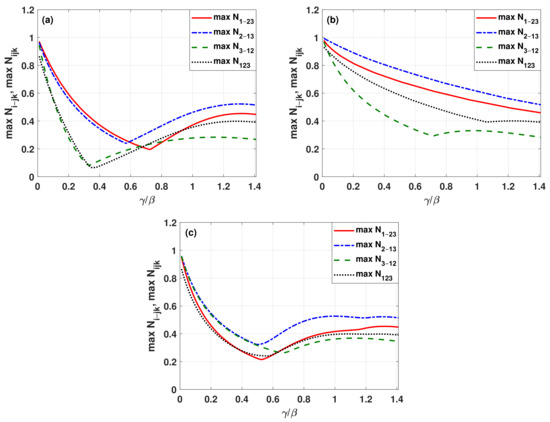
Figure 6. Maximal values of bipartite ($N_{i-jk}$) and tripartite ($N_{ijk}$) negativities versus $\gamma /\beta$ for $\omega =5\beta$ and for various initial states $\widehat{\rho }(t=0)$: (a) $|100⟩⟨100|$, (b) $|010⟩⟨010|$, (c) $|001⟩⟨001|$.

In the next analyzed case, at the beginning of the time evolution of the system, only the neutral cavity is excited. We can see (in Figure 6b) that for very small values of ratio $\gamma /\beta$, all bipartite negativities $N_{i-jk}$ are approximately equal to unity while the tripartite negativity $N_{123}$ is slightly smaller. When the value of the loss/gain parameter $\gamma$ increases, the strength of bipartite entanglements between 1−23 and 2−13 gradually decreases. The tripartite entanglement and the bipartite entanglement between 3−12 initially decrease to their minima and then gradually increase to a certain value, then slightly decrease again, when the ratio $\gamma /\beta$ is close to the phase transition point. For all values of $\gamma /\beta$ in the unbroken phase of $\mathcal{PT}$-symmetry, the bipartite entanglement between 2−13 is always the strongest, while the weakest one is the entanglement between 3−12.

In the last case, the active cavity will be excited, while the others will remain in a vacuum state. The changes in the maximal values of bipartite and tripartite negativities are illustrated in Figure 6c. We can see that when we increase the ratio of $\gamma /\beta$ while remaining in the unbroken phase of $\mathcal{PT}$-symmetry, the tripartite entanglement and all bipartite entanglements between subsystems initially decrease to their minima and then increase again to their local maxima. After that, they slightly decrease and increase again. These changes after reaching $\gamma /\beta =1$ are quite small in comparison to the overall changes of those functions. Although all entanglement measures differ in values, they follow the same kind of shape, and thus they are closer to each other than in the first two scenarios. For all ratios of $\gamma /\beta$ in the unbroken phase, the bipartite entanglement between 2−13 is always the strongest. Among all bipartite measures $N_{i-jk}$, the lowest value of entanglement is achieved for subsystem pair 1−23. As the changes of negativities start to stabilize, the entanglement between 3−12 becomes the weakest one.

In Figure 5a,c,e, the same as in Figure 2a,c,e, we see that the entanglements disappear in time, and the strongest entanglements are generated at the initial time of evolution. This decrease is related to the growth of the number of states that are populated. However, after a sufficiently long time, the situation stabilizes, and we achieve an equilibrium between the inflow and outflow of energy. Then the negativities values do not change with time, and we obtain a stable entanglement. Such a stabilization, we can observe faster when the gamma parameter reaches higher values. With the increase in the values of gamma, a larger group of three-mode states is populated faster, so the maximal negativities are smaller, and the generated entanglements are weaker (see Figure 2b,d,f and Figure 5b,d,f). For small values of the gain/loss parameter, the entanglements appear in the subspace defined by the states $|0⟩$ and $|1⟩$. With an increase in the parameter gamma, the strength of entanglement decreases what is related to the growth of the number of populated states. However, with a further increase in the gamma, we observe the increase of maximal values of negativities (see Figure 3 and Figure 6). Such behavior is correlated with the appearance of entanglements related to states $|0⟩$ and $|2⟩$, and the disappearance of entanglements related to states $|0⟩$ and $|1⟩$.

In Figure 7, we present the tripartite entanglement of our system’s steady-state solution for various ratios of $\gamma /\beta$. Similarly to Figure 2, we notice that for small values of $\gamma /\beta$ and time $t\to \infty$, all bipartite ($i-jk$) entanglements and thus the tripartite entanglement are not generated. As previously, when we increase the ratio $\gamma /\beta$, the entanglements start to appear. However, in this case, all values of negativities become nonzero. We see that by increasing the value of $\gamma /\beta$, we can produce stable entangled states even when the ratio $\gamma /\beta$ converges towards the phase transition point. Among all bipartite entanglements ($i-jk$), the entanglement between 2−13 always remains the strongest, while the entanglement between 3−12 is the weakest for all considered values of $\gamma /\beta$. Moreover, the negativity $N_{123}$ reaches a value of $0.4$, which is higher than for the negativities $N_{ij}$ presented in Figure 4.

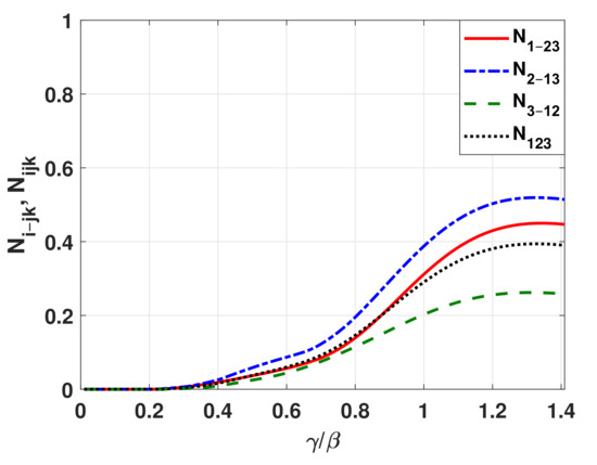
Figure 7. Steady-state solutions for the negativities (full tripartite $N_{123}$ and bipartite $N_{i-jk}$) versus the value of the ratio $\gamma /\beta$ for $\omega =5\beta$.

4. Conclusions

In this paper, we have discussed a $\mathcal{PT}$-symmetric system that consists of three optical resonant elements coupled together. This so-called optical trimer composed of three cavities characterized by the same resonant frequency formed a chain. The first and third cavities were related to the loss and gain of energy, respectively. Moreover, the strength of interaction between these cavities and the neutral cavity was set to be equal. For various initial scenarios and parameters of the system, we investigated quantum correlations by calculating bipartite and tripartite negativities as quantifiers of entanglement. To ensure that we are in the $\mathcal{PT}$-symmetric unbroken phase, we limited ourselves to parameters obeying the relation $\gamma <\sqrt{2}\beta$. In our analysis, we have tuned the gain/loss parameter $\gamma$ to examine the generation of bipartite and tripartite entanglements, leaving the coupling parameter $\beta$ constant and equal to one. We distinguished three various initial states of the system. Those initial states were situations when one of the three possible cavities was excited, while the others remained in a vacuum state. In each such case, we examined the impact of the ratio between the gain/loss parameter and the coupling parameter ($\gamma /\beta$) on the bipartite and tripartite entanglements. In all analyzed scenarios, we have found that the strength of bi- and tripartite entanglement not only strongly depends on the value of $\gamma /\beta$ but also on the initial state of the system. The time evolution of all negativities for all initial states and small values of the ratio $\gamma /\beta =0.01$ is periodical. The amplitudes of those oscillations decrease over time. On the other hand, for the ratio $\gamma /\beta =0.8$, the oscillations disappear, and after some initial fluctuations, the evolutions of negativities converge fast to constant values. We also calculated and presented, for all initial cases, the maximal values of bipartite negativities concerning the parameter $\gamma /\beta$. We have noticed that the entanglement between subsystems 1−3 for $\gamma /\beta$ is significantly stronger in the second case, which is when initially the neutral cavity is excited. Moreover, in the first two situations when the passive or neutral cavities are excited, we have shown that the entanglement between 1−2 is higher than between 2−3 for all permissible values of $\gamma /\beta$. This tendency is completely reversed in the last case when the active cavity is excited. Subsequently, we analyzed the evolution of tripartite entanglement for all three initial states and two values of $\gamma /\beta$, namely, for $\gamma /\beta =0.01$ and $\gamma /\beta =0.8$. Similarly to the analysis for the bipartite entanglements, we have noticed periodical oscillations with damping of the tripartite entanglement over time, for $\gamma /\beta =0.01$. Moreover, the highest tripartite entanglement can be observed for the case when the neutral cavity is initially excited. In the case of $\gamma /\beta =0.8$, we see that again, the oscillations disappeared, and after initial fluctuations, the tripartite negativities converge to constant values over time. Here, the highest value of tripartite negativity was observed at the beginning of the time evolution for the neutral cavity. Finally, we analyzed the maximal values of tripartite negativity for the ratio of $\gamma /\beta$ for the three initial states. We have seen that again the highest tripartite entanglement is created in the situation when the neutral cavity is initially excited. To investigate the behavior of bi- and tripartite entanglements for unlimited time and various gain/loss parameter $\gamma$, we analyzed the dependence of steady-state entanglements on the ratio $\gamma /\beta$. We have realized that all bi- and tripartite entanglements are not generated for very small values of $\gamma /\beta$. When we increase the value of $\gamma /\beta$, except for the slow rise of bipartite entanglement between 1−3, all other bi- and tripartite entanglements begin to appear and increase their strength quite rapidly. Even when the value of $\gamma /\beta$ is close to the phase transition point, bi- and tripartite entanglements are still generated. Finally, to investigate the behavior of bipartite and tripartite entanglement in the context of various values of the ratio $\gamma /\beta$ and the long time limit, we have calculated the steady-state solutions. Importantly, it turns out that for large enough ratios of $\gamma /\beta$, we can observe a quite strong entanglement. This is an important result since we obtain the desired and strong entanglement after our system stabilizes by applying a high enough value of $\gamma$. This observation refers to both bipartite and tripartite entanglements.

Summarizing, we have shown that the entanglement generation in a physical system consisting of three optical resonant elements coupled together strongly depends on the ratio of gain and loss parameter $\gamma$ and coupling parameter $\beta$. For higher values of this ratio, the negativity values stabilize around lower but noticeable values. Most importantly, for the ratio $\gamma /\beta >1.2$, we can achieve a high degree of entanglement in steady-state solutions for not only bipartite but also tripartite negativity.

References

- Bender, C.M.; Boettcher, S. Real Spectra in Non-Hermitian Hamiltonians Having PT Symmetry. Phys. Rev. Lett. 1998, 80, 5243–5246. [Google Scholar] [CrossRef]
- Bender, C.M.; Brody, D.C.; Jones, H.F. Complex Extension of Quantum Mechanics. Phys. Rev. Lett. 2002, 89, 270401. [Google Scholar] [CrossRef] [PubMed]
- Bender, C.M. Making sense of non-Hermitian Hamiltonians. Rep. Prog. Phys. 2007, 70, 947. [Google Scholar] [CrossRef]
- Bender, C.M.; Gianfreda, M.; Ozdemir, C.K.; Peng, B.; Yang, L. Two fold transition in PT -symmetric coupled oscillators. Phys. Rev.A 2013, 88, 062111. [Google Scholar] [CrossRef]
- Wrona, I.A.; Jarosik, M.W.; Szczęśniak, R.; Szewczyk, K.A.; Stala, M.K.; Leoński, W. Interaction of the hydrogen molecule with the environment: Stability of the system and the PT symmetry breaking. Sci. Rep. 2020, 10, 215. [Google Scholar] [CrossRef]
- Feng, L.; Xu, Y.; Fegadolli, W.S.; Lu, M.; Oliveira, J.E.B.; Almeida, V.R.; Chen, Y.; Scherer, A. Experimental demonstration of a unidirectional reflectionless parity-time metamaterial at optical frequencies. Nat. Mater. 2013, 12, 108–113. [Google Scholar] [CrossRef]
- Guo, A.; Salamo, G.J.; Duchesne, D.; Morandotti, R.; Volatier-Ravat, M.; Aimez, V.; Siviloglou, G.A.; Christodoulides, D.N. Observation of PT-Symmetry Breaking in Complex Optical Potentials. Phys. Rev. Lett. 2009, 103, 093902. [Google Scholar] [CrossRef]
- Peng, B.; Özdemir, C.K.; Rotter, S.; Yilmaz, H.; Liertzer, M.; Monifi, F.; Bender, C.; Nori, F.; Yang, L. Loss-induced suppression and revival of lasing. Science 2014, 346, 328–332. [Google Scholar] [CrossRef]
- Hodaei, H.; Miri, M.A.; Heinrich, M.; Christodoulides, D.N.; Khajavikhan, M. Parity-time–symmetric microring lasers. Science 2014, 346, 975–978. [Google Scholar] [CrossRef]
- Jing, H.; Özdemir, S.K.; Lü, X.Y.; Zhang, J.; Yang, L.; Nori, F. PT-Symmetric Phonon Laser. Phys. Rev. Lett. 2014, 113, 053604. [Google Scholar] [CrossRef]
- He, B.; Yang, L.; Xiao, M. Dynamical phonon laser in coupled active-passive microresonators. Phys. Rev. A 2016, 94, 031802. [Google Scholar] [CrossRef]
- Bittner, S.; Dietz, B.; Günther, U.; Harney, H.L.; Miski-Oglu, M.; Richter, A.; Schäfer, F. PT Symmetry and Spontaneous Symmetry Breaking in a Microwave Billiard. Phys. Rev. Lett. 2012, 108, 024101. [Google Scholar] [CrossRef] [PubMed]
- Liu, Y.; Hao, T.; Li, W.; Capmany, J.; Zhu, N.; Li, M. Observation of parity-time symmetry in microwave photonics. Light. Sci. Appl. 2018, 7. [Google Scholar] [CrossRef] [PubMed]
- Suchkov, S.V.; Fotsa-Ngaffo, F.; Kenfack-Jiotsa, A.; Tikeng, A.D.; Kofane, T.C.; Kivshar, Y.S.; Sukhorukov, A.A. Non-Hermitian trimers: PT-symmetry versus pseudo-Hermiticity. New J. Phys. 2016, 18, 065005. [Google Scholar] [CrossRef]
- Suchkov, S.V.; Sukhorukov, A.A.; Huang, J.; Dmitriev, S.V.; Lee, C.; Kivshar, Y.S. Nonlinear switching and solitons in PT-symmetric photonic systems. Laser Photonics Rev. 2016, 10, 177–213. [Google Scholar] [CrossRef]
- Kawabata, K.; Ashida, Y.; Katsura, H.; Ueda, M. Parity-time-symmetric topological superconductor. Phys. Rev. B 2018, 98, 085116. [Google Scholar] [CrossRef]
- Kremer, M.; Biesenthal, T.; Heinrich, M.; Thomale, R.; Szameit, A. Demonstration of a two-dimensional PT-symmetric crystal: Bulk dynamics, topology, and edge states. Nat. Commun. 2019, 10. [Google Scholar] [CrossRef]
- Zhou, L.; Gong, Z.; Liu, Y.x.; Sun, C.; Nori, F. Controllable scattering of a single photon inside a one-dimensional resonator waveguide. Phys. Rev. Lett. 2008, 101, 100501. [Google Scholar] [CrossRef]
- Wang, Z.H.; Li, Y.; Zhou, D.L.; Sun, C.P.; Zhang, P. Single-photon scattering on a strongly dressed atom. Phys. Rev. A 2012, 86, 023824. [Google Scholar] [CrossRef]
- Wang, Z.H.; Zhou, L.; Li, Y.; Sun, C.P. Controllable single-photon frequency converter via a one-dimensional waveguide. Phys. Rev. A 2014, 89, 053813. [Google Scholar] [CrossRef]
- Xu, X.W.; Liu, Y.X.; Sun, C.P.; Li, Y. Mechanical symmetry in coupled optomechanical systems. Phys. Rev. A 2015, 92, 013852. [Google Scholar] [CrossRef]
- Li, J.; Yu, R.; Wu, Y. Proposal for enhanced photon blockade in parity-time-symmetric coupled microcavities. Phys. Rev. A 2015, 92, 053837. [Google Scholar] [CrossRef]
- Chang, L.; Jiang, X.; Hua, S.; Yang, C.; Wen, J.; Jiang, L.; Li, G.; Wang, G.; Xiao, M. Parity–time symmetry and variable optical isolation in active–passive-coupled microresonators. Nat. Photonics 2014, 8, 524–529. [Google Scholar] [CrossRef]
- Kalaga, J.K. The Entanglement Generation in -Symmetric Optical Quadrimer System. Symmetry 2019, 11, 1110. [Google Scholar] [CrossRef]
- Xue, L.; Gong, Z.; Zhu, H.; Wang, Z. PT symmetric phase transition and photonic transmission in an optical trimer system. Opt. Express 2017, 25, 17249–17257. [Google Scholar] [CrossRef]
- Peres, A. Separability Criterion for Density Matrices. Phys. Rev. Lett. 1996, 77, 1413–1415. [Google Scholar] [CrossRef]
- Horodecki, M.; Horodecki, P.; Horodecki, R. Separability of mixed states: Necessary and sufficient conditions. Phys. Lett. A 1996, 223, 1–8. [Google Scholar] [CrossRef]
- Sabín, C.; Garcia-Alcaíne, G. A classification of entanglement in three-qubit systems. Eur. Phys. J. D. 2008, 48, 435–442. [Google Scholar] [CrossRef]
Publisher’s Note: MDPI stays neutral with regard to jurisdictional claims in published maps and institutional affiliations. |
© 2021 by the authors. Licensee MDPI, Basel, Switzerland. This article is an open access article distributed under the terms and conditions of the Creative Commons Attribution (CC BY) license (http://creativecommons.org/licenses/by/4.0/).