Abstract
Zero watermarking is an important part of copyright protection of vector geographic data. However, how to improve the robustness of zero watermarking is still a critical challenge, especially in resisting attacks with significant distortion. We proposed a zero watermarking method for vector geographic data based on the number of neighboring features. The method makes full use of spatial characteristics of vector geographic data, including topological characteristics and statistical characteristics. First, the number of first-order neighboring features (NFNF) and the number of second-order neighboring features (NSNF) of every feature in vector geographic data are counted. Then, the watermark bit is determined by the NFNF value, and the watermark index is determined by the NSNF value. Finally, combine the watermark bits and the watermark indices to construct a watermark. Experiments verify the theoretical achievements and good robustness of this method. Simulation results also demonstrate that the normalized coefficient of the method is always kept at 1.00 under the attacks that distort data significantly, which has the superior performance in comparison to other methods.
1. Introduction
Vector geographic data is one of the most important production materials in information society [1]. It is an inevitable requirement to ensure the security of vector geographic data in order to develop geographic information systems (GIS) industries. As a frontier technology for information security, digital watermarking plays a critical role in copyright protection and content authentication of vector geographic data [2,3,4,5,6]. Particularly in terms of copyright protection, zero watermarking has gained more and more attention. It is a kind of watermarking technology that does not cause any modification to the host data [7]. Zero watermarking constructs watermark by means of quantifying the characteristics of the data and then registers the watermark and additional information to a third-party intellectual property rights (IPR) repository. Therefore, compared with the traditional embedding watermarking [8], zero watermarking has no damage to data accuracy, which can be applied for vector geographic data with high-precision requirements. It balances the contradiction between the invisibility and the robustness of watermarking [9]. The robustness of watermarking refers to the ability to detect the watermark information from watermarked data after being attacked [10,11]. However, there are many kinds of attacks for vector geographic data, such as geometrical attacks, vertex attacks, and object attacks [12,13]. These attacks will damage data from different perspectives, thereby affecting the synchronization of watermark information. It puts forward higher demands for the robustness of zero watermarking. Thus, how to improve the robustness is a hotspot in the current research of zero watermarking for vector geographic data.
The existing zero watermarking methods for vector geographic data can be divided into two types. The first type is the method based on attribute characteristics [14,15,16,17]. It quantifies the descriptive information of vector geographic data (such as what, why, and when) to construct a zero watermark. For example, scholars select element coding [14], stroke width [15], color [16], and map symbols [17] as the attribute characteristic. If the attribute information is of a numeric type, it can be directly quantified to watermark information. If it is of a text type, some approaches of converting text to numbers need to be used, such as encoding and statistics. Generally, this type of method has strong robustness and can perfectly resist geometrical attacks, including rotation, scaling, and translation (RST) attacks. This is because RST attacks only change coordinates, not attributes. However, the method has high requirements for the integrity of the attributes. Only the vector geographic data whose attributes meet certain conditions can implement watermark embedding. Moreover, the attribute information of vector geographic data differs from the production stage and the application scenario. Therefore, this type of method has significant application limitations.
The second type is the method based on spatial characteristics [8,9,18,19,20,21,22,23,24,25,26,27,28,29,30,31,32]. It quantifies the coordinates of vector geographic data to construct the zero watermark. There are two ways to use coordinates. One is to use the coordinate directly. For example, literature [21] compares the coordinates of vertices to obtain a Boolean sequence and then quantify the sequence to a watermark that contains only zero and one. Literatures [9,18,24] count the number of vertices that meet certain spatial location conditions. Another is to use the coordinate indirectly. For example, scholars employ the angle [8,19,20,29,30,31,32], distance [25,26], distance ratio [22,27], and topology [28] to construct a watermark, respectively. Compared with attribute characteristics, spatial characteristics are the basis of vector geographic data. Therefore, the method based on spatial characteristics solves the application limitation of the first type. Besides, most of them can resist common geometrical attacks. However, the watermark synchronization of this method is strongly coupled with the coordinates, so it is difficult to resist the attacks with significant distortion, such as non-uniform scaling and projection transformation attacks.
Through the above analysis, it is found that the method based on attribute characteristics is robust to attacks related to coordinates but has many limitations in practical applications. The method based on spatial characteristics solves the issues of the former and can resist common geometrical attacks, but it is difficult to resist attacks that have significant distortion on the data. Therefore, how to find the characteristics that can completely resist data deformation is a critical scientific problem.
To resolve the above problem, we propose a zero watermarking algorithm based on the number of neighboring features for vector geographic data. It changes the target of statistics from vertices to features and is fully integrated with topological relationships between features. The remainder of this paper is organized as follows. Section 2 gives the basic ideas and details of the algorithm. The experimental design is described in Section 3. Then Section 4 provides corresponding experimental results and analyses, and Section 5 gives some discussions. Finally, Section 6 draws the conclusion.
2. Methodology
The proposed method is based on the number of neighboring features of vector geographic data. Specifically, the polygon data is used as the watermarking target in this paper. For a polygon, it has first-order neighbors, that is, the polygons that are neighbors directly to the polygon. At the same time, it also has second-order neighbors that refer to neighbors of neighbors. The key to the method is how to use the number of neighboring features. Firstly, the number of first-order neighboring features (referred to as NFNF hereafter) and the number of second-order neighboring features (referred to as NSNF hereafter) are counted for every feature. Then, NFNF is quantified as the watermark bit, and NSNF is quantified to the watermark index. The watermark index represents the mapping relationship between the feature and the watermark bit. Finally, the watermark is constructed by combining the watermark indices and the watermark bits. Figure 1 shows the basic idea of the algorithm. The final constructed watermark can be encrypted with a secret key to enhance the security of the method. For example, the literature [28] uses a logistic mapping model to encrypt the watermark information. That is, the proposed method can be combined with the encryption method. This paper focuses on the procedure of constructing the zero watermark, so we do not integrate any encryption operations in the method.
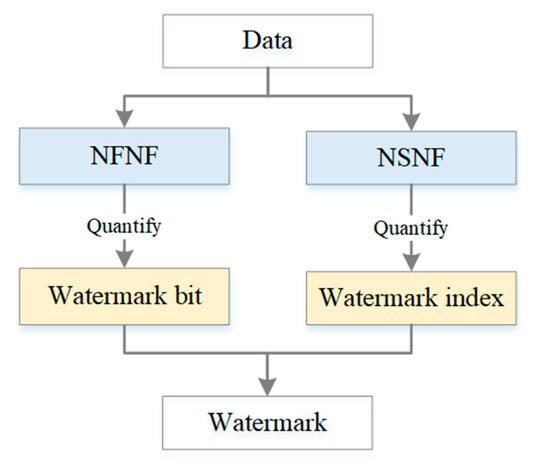
Figure 1.
The basic idea of the proposed method.
2.1. Neighboring Features
The neighboring relationships can be divided into three types for polygons: (1) Overlapping neighbors: polygons that have all or part of their areas overlapping; (2) Edge neighbors: polygons that have common or touching boundaries; (3) Node neighbors: polygons that touch at a point (https://desktop.arcgis.com/en/arcmap/latest/tools/analysis-toolbox/how-polygonneighbors-analysis-works.htm). Polygon A and polygon B demonstrate these three types of neighboring relationships in Figure 2. In the proposed method, if two features belong to any of the three types, they will be regarded as neighbors.
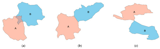
Figure 2.
Three types of neighbors: (a) Overlapping neighbors; (b) Edge neighbors; (c) Node neighbors.
Figure 3 demonstrates the statistics of neighboring features based on the above three neighboring relationships. Figure 3a shows the statistics of NFNF values, and the number in each polygon is its corresponding NFNF value. Similarly, Figure 3b shows the statistics of NSNF values. For a polygon, its NSNF is the sum of the NFNFs of all its neighbors and is calculated by the following equation.
where n is the NFNF of a polygon and means the NFNF of its i-th neighbor.
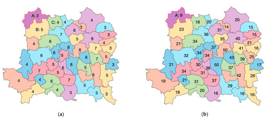
Figure 3.
The statistics of neighboring features: (a) NFNF values; (b) NSNF values.
In Figure 3, take polygon A in the upper left corner as an example. From Figure 3a, it is easy to see that polygon A has two neighbors: B and C, so the NFNF of polygon A is 2. Then, polygon B and polygon C have five and four neighbors separately, so the NSNF of polygon A is 9, as shown in Figure 3b. Clearly, the NSNF value is larger than the NFNF value for a polygon. Therefore, using the NSNF to quantify the watermark index can make the distribution of the watermark index more uniform.
2.2. The Determination of the Watermark Bit
In this paper, the watermark is a binary sequence with a fixed length [27]. Every watermark bit is zero or one. The watermark bit of a polygon is determined by quantizing its NFNF. The quantization is a process of mapping input values from a large set to output values in a smaller set. We use the following equation to quantify the NFNF.
where Mod is the modulo operation.
2.3. The Determination of the Watermark Index
Similar to the determination of the watermark bit, the watermark index is obtained by quantizing the NSNF. Set the length of the watermark to N, so the watermark index of a polygon ranges from 1 to N. It can be calculated by the following equation.
where Rand is a random number generator that creates uniformly distributed pseudorandom integers between 1 and N. The first parameter of Rand is the seed or start value of the random number generator.
The watermark index of a polygon presents the position of its watermark bit in the final zero watermark. There will be a situation that the watermark indices of multiple polygons are the same. Then, the majority voting mechanism [12] is employed to determine the watermark bit on the watermark index. For a watermark index, if the number of watermark bit 1 is larger than that of watermark bit 0, the watermark bit will be recorded as 1. Otherwise, the watermark bit will be recorded as 0.
2.4. Watermark Generation and Extraction
In the proposed method, the watermark generation and the watermark extraction are exactly the same processes. However, they happen at different times. The watermark generation occurs in the initial stage of the algorithm to generate a watermark. However, the watermark extraction is executed when copyright infringement needs to be confirmed, which generates a watermark from suspicious data and identifies the watermark by comparing it with the watermark registered in the IPR repository.
Denote the polygon data as , presents the polygon in i-th position by storage, and M is the total number of polygons. Firstly, count the NFNF and NSNF of . Then, get the watermark bit and the watermark index of according to Equations (2) and (3). The set of watermark bits is denoted by , and the set of watermark indices is denoted by . Next, introduce a set that all the elements are 0, denoted by . Reassign the value of by the following equation:
Finally, construct the zero watermark by Equation (5) and denote it as .
3. Experiments
3.1. Datasets
To evaluate the performance of the proposed method, we choose the administrative divisions of an area in China as our datasets. The data format of the datasets is shapefile, which is a common geospatial vector data format for GIS applications. Its projected coordinate system is Gauss Kruger, in which the datum is Beijing 1954 and the unit is the meter (m). The bounds in the x-axis and y-axis are [, ] and [, ], separately. As shown in Figure 4, there are 729 features and 152701 vertices in the experimental data.
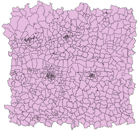
Figure 4.
The experimental data.
3.2. Experiment Design and Implementation
This section is to set up attack experiments with different types and intensities to verify the robustness of the proposed method. The following attack types are selected, as shown in Table 1. Some attacks will cause significant distortion in the data, such as non-uniform scaling in geometrical attacks, simplification in vertex attacks, and most projection transformation attacks. If an algorithm can resist the above attacks, it is proved that the algorithm solves the scientific problem of this article. That is, the algorithm finds the characteristics that can completely resist data deformation. The rest of the attacks are also common attacks in geographic analysis, and a qualified digital watermarking algorithm should be able to resist them. Detailed settings for every type of attack will be given later.

Table 1.
The types of attack experiments.
Meanwhile, two algorithms are selected for comparison, referred to as Wang [24] and Li [28] separately. They are the representatives of the method based on spatial characteristics. The former uses coordinate directly. It constructs concentric rings and then quantifies the number of vertices in each ring to obtain a zero watermark. The latter uses coordinates indirectly. Firstly, it builds the graphical complexity index of the polygon, then calculates the spatial correlation coefficient based on the graphical complexity index. Finally, it quantizes the coefficients to obtain a zero watermark.
3.2.1. Geometrical Attacks
Generally, geometrical attacks include RST attacks. In particular, scaling attacks can be categorized into uniform scaling and non-uniform scaling. Uniform scaling means that the scaling factors in the x and y directions, denoted as Sx and Sy, are the same, while Sx is not equal to Sy in non-uniform scaling. In rotation attacks, the data is rotated clockwise with the data center by a rotation angle from 0° to 360° with the step of 60°. In scaling attacks, the data is scaled with respect to the data center by scale factors: 0.4, 0.6, 0.8, 2, 3, and 4. For translation attacks, the data is translated by a distance, denoted by translation distance, at the same time in x and y directions. The translation distance ranges from 0 m to 600 m with a gap of 100 m. Some results after attacks are shown in Figure 5. One can see that non-uniform scaling in Figure 5d makes the shape of the features deformed.
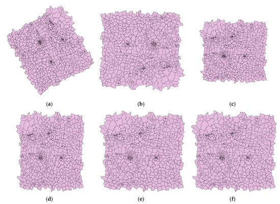
Figure 5.
The data after geometrical attacks: (a) Rotation angle = 60°; (b) Rotation angle = 180°; (c) Sx = 0.8, Sy = 0.8; (d) Sx = 0.8, Sy = 1; (e) Translation distance = 100 m; (f) Translation distance = 200 m.
3.2.2. Vertex Attacks
In this paper, vertex attacks include interpolation and simplification, which change the number of vertices in the data. In interpolation attacks, we use linear interpolation to insert vertices between adjacent vertices. When the distance between the x-coordinates or y-coordinates of adjacent vertices is greater than the defined tolerance (refers to interpolation tolerance), a new vertex will be inserted between the adjacent vertices. The interpolation tolerance ranges from 0 m to 600 m with the step of 100 m. On the contrary, simplification attacks remove vertices from the data, in which the Douglas–Peucker algorithm [12] is used. The simplification tolerance also ranges from 0 m to 600 m with the step of 100 m. Figure 6 shows the results after interpolation and simplification when the tolerance is 600 m, and the ones on the right are partial enlargements of the left. It is easy to see that the shape of the features in Figure 6b is greatly distorted in comparison to Figure 6a.
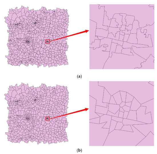
Figure 6.
The data after vertex attacks: (a) Interpolation tolerance = 600 m; (b) Simplification tolerance = 600 m.
3.2.3. Object attacks
Object attacks in this paper include object addition and object deletion. The feature, as the minimum operating unit, is added or deleted in the data. Therefore, the number of features changes, but the shape of the features does not. In experiments, features are added or deleted sequentially from the bottom of the original data. Both the addition ratio and the deletion ratio range from 0% to 30% of the number of original features, with the step of 5%. Some visualization results after object attacks are shown in Figure 7.
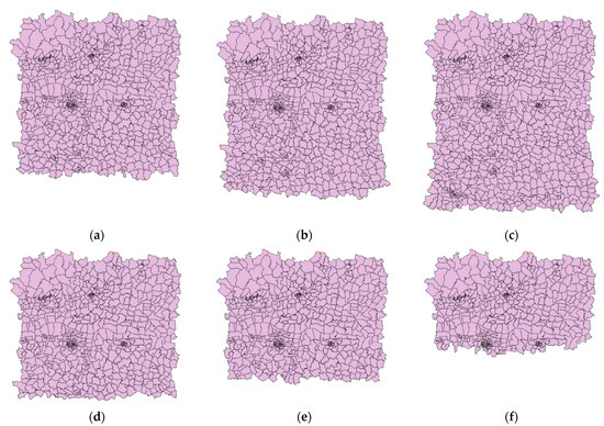
Figure 7.
The data after object attacks: (a) Addition ratio = 5%; (b) Addition ratio = 15%; (c) Addition ratio = 30%; (d) Deletion ratio = 5%; (e) Deletion ratio = 15%; (f) Deletion ratio = 30%.
3.2.4. Projection Transformation Attacks
Projection transformation is a process of projecting spatial data from one coordinate system to another [33]. Since the experimental data in this paper have a projected coordinate system, two types of projection transformation attacks are set. The first is from projected coordinate systems to geographic coordinate systems, in which three geographic coordinate systems are selected: Beijing 1954, Xian 1980, and China Geodetic Coordinate System (CGCS) 2000, numbered 1, 2, and 3. The second is from projected coordinate systems to other projected coordinate systems. We also choose three projected coordinate systems: cylindrical equal area, Lambert conformal conic and azimuthal equidistant, numbered 4, 5, and 6. The results after projection transformation attacks are shown in Figure 8. It is easy to see that except for Figure 8e, the shape of features is distorted substantially.
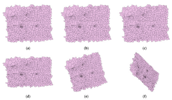
Figure 8.
The data after projection transformation attacks: (a) To Beijing 1954; (b) To Xian 1980; (c) To CGCS 2000; (d) To cylindrical equal area; (e) To Lambert conformal conic; (f) To azimuthal equidistant.
3.3. Evaluation
After extracting the zero watermark from the suspicious data, we need to compare it with the zero watermark W that registered in the IPR repository. Normalized correlation (NC) is employed to evaluate the quality of the extracted results, and it is one of the most common evaluation methods [34]. The mathematical equation of NC is as follows:
where N is the length of the watermark. NC ranges from 0 to 1, and the larger the NC, the greater the correlation between the extracted watermark and the registered watermark. In addition, the threshold of NC is introduced, which is an empirical value. When the NC is greater than the threshold, the watermark detection succeeds. Otherwise, it is considered a failure. In the proposed method, we set the length of watermark N to 32 and the threshold of NC to 0.75.
4. Results and Analyses
4.1. The Results of Geometrical Attacks
Figure 9, Figure 10, Figure 11 and Figure 12 show the results of geometrical attacks. Overall, three algorithms perform equally well in rotation, uniform scaling and translation attacks, where their NC values are all 1.00. However, in non-uniform scaling attacks, the differences between the three algorithms are obvious. As shown in Figure 11, Sx increases from 0.4 to 4, while Sy remains at 1. Therefore, from (0.4,1) to (1,1), the shape of features recovers from the flattened state in the x direction. However, from (1,1) to (4,1), the shape is elongated in the x direction. It can be observed that the NC values of the proposed method always keep 1.00, while that of Wang and Li increases and then decreases. Especially when the scaling factor is (0.4,1), (3,1) and (4,1), the NC values of Li fall below the threshold value, 0.75. Thus, it is proved that the proposed method can resist geometrical attacks completely.
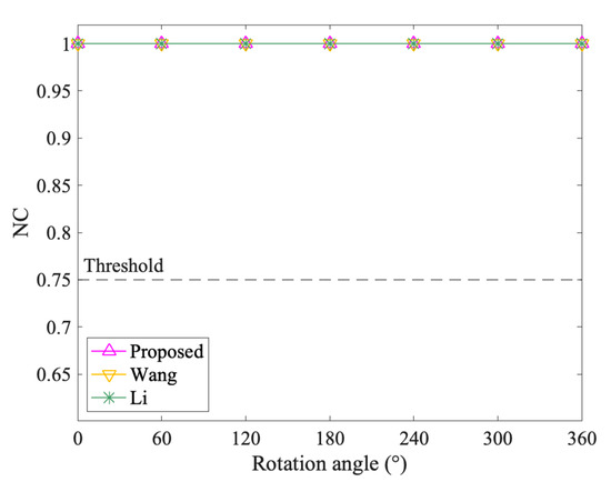
Figure 9.
The results after rotation attacks.
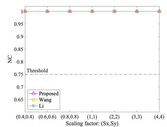
Figure 10.
The results after uniform scaling attacks.
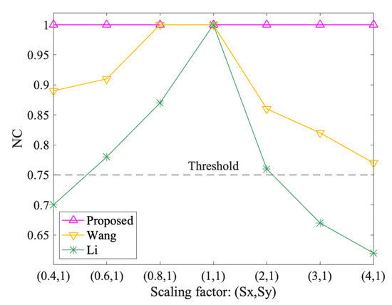
Figure 11.
The results after non-uniform scaling attacks.
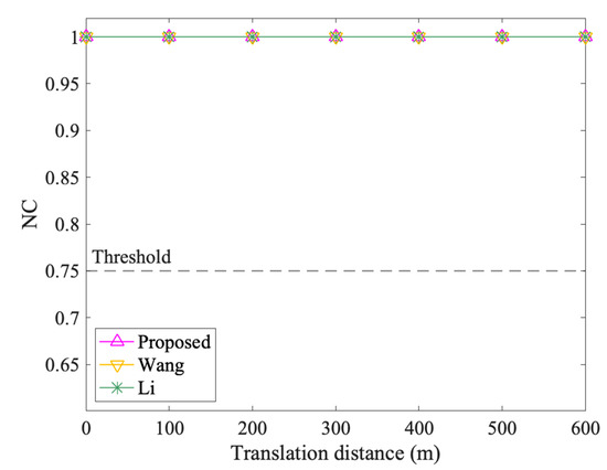
Figure 12.
The results after translation attacks.
4.2. The Results of Vertex Attacks
Figure 13 and Figure 14 show the results of vertex attacks. The NC values of the proposed algorithm are always 1.00 in interpolation and simplification attacks, while the values of Li and Wang vary. In interpolation attacks, Li’s algorithm performs the same as the proposed method. When the interpolation tolerance is 100 m, the NC value of Wang decreases from 1.00 to 0.97, but it keeps at 0.97 afterward. In the simplified attack, the NC values of Wang and Li both showed a downward trend. However, compared to Wang, Li dropped more. For example, when the Simplification tolerance is 600 m, the NC values of Wang and Li are 0.92 and 0.87, respectively. In short, the proposed method performs better and is not affected by interpolation and simplification attacks.
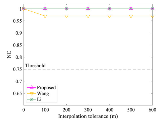
Figure 13.
The results after interpolation attacks.
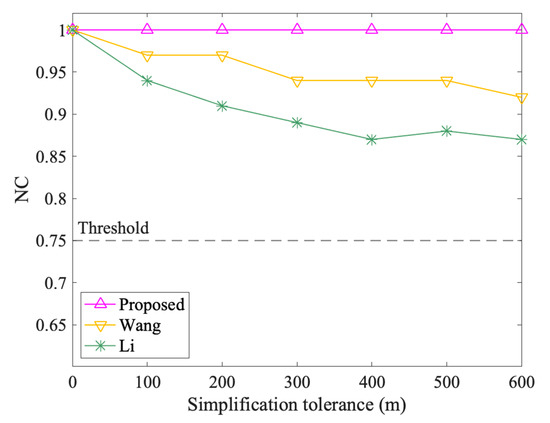
Figure 14.
The results after simplification attacks.
4.3. The Results of Object Attacks
The results of object attacks are shown in Figure 15 and Figure 16. The NC values of the three methods all change with different addition and deletion ratios. In object addition attacks, both the proposed method and Wang tend to decrease first and then increase, in which their lowest values are 0.87 and 0.97, separately, and Wang performs better. However, Li’s NC value keeps decreasing, especially when the addition ratio is 30%, the NC value drops to 0.76, which is slightly higher than the threshold. In object deletion attacks, the three algorithms all show an overall downward trend. Wang’s ups and downs are large, the proposed method is relatively flat, but both are above the threshold. Li also keeps dropping, but when the deletion ratio exceeds 20%, the NC value falls below the threshold. Overall, the performance ranking of the three is that Wang is better than the proposed algorithm, and the proposed algorithm is better than Li. Since the NC values of the proposed method are always above the threshold, the method can resist object attacks.
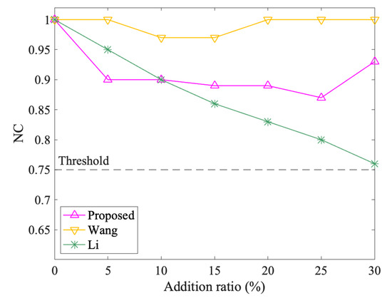
Figure 15.
The results after object addition attacks.
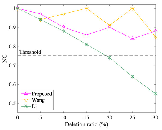
Figure 16.
The results after object deletion attacks.
4.4. The Results of Projection Transformation Attacks
Figure 17 shows the results of projection transformation attacks. Overall, the NC value of the proposed method maintains at 1.00, while that of Wang and Li is less than 1.00 except when the projection transformation number is 5. As mentioned in Section 3.2.4, projection transformation number 5 refers to projecting the data to Lambert conformal conic projection, where the shape of features does not change much. However, the shape of the features is distorted in other projection transformation attacks. The minimum NC values of Wang and Li are 0.92 and 0.73, respectively, when the projection transformation numbers are 4 and 6. Therefore, the proposed algorithm performs best, which shows that it can resist projection transformation attacks completely.
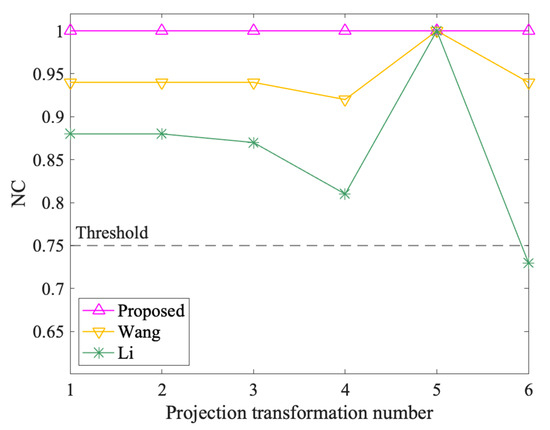
Figure 17.
The results after projection transformation attacks.
5. Discussions
The above experimental results suggest that the proposed method has strong robustness under various attacks, especially for attacks with significant distortion, such as non-uniform scaling attacks, simplification attacks, and projection transformation attacks. Further discussions will be given from three perspectives to understand the characteristics of the proposed method better.
5.1. Local Characteristics
NFNF and NSNF are the foundation of the proposed method to construct the zero watermark. Based on neighbors, the former determines the watermark bit. Based on neighbors of neighbors, the latter determines the watermark index. Therefore, both of them reflect the local characteristics of the vector geographic data. This is why the proposed method can resist object attacks. When a feature is added or deleted in vector geographic data, this only affects one local part of the data, while some parts can be retained without being damaged. That is, the watermark in these unattacked parts is preserved and can be detected successfully.
Meanwhile, NFNF and NSNF are based on statistics of features, not vertices. Compared with vertices, the characteristics of the two are not so particularly local, but they are just right. This is the core reason why the proposed method can resist vertex attacks. In vertex attacks, the interpolation and simplification of vertices do not affect the neighboring relationship between features in vector geographic data, which is verified by Figure 13 and Figure 14. In the two figures, with the addition and deletion of vertices, the NC value of the proposed method is always kept at 1.00. Thus, the two local characteristics, NFNF and NSNF, enhance the robustness of the proposed algorithm.
5.2. Applied to Polyline Data
The algorithm in this paper is used for polygon data because it is based on the number of neighboring polygons. However, only with some simple modifications, the method can also be applied to polyline data. The key idea is to change the topological relationship from the adjacency to the intersection when counting the number of neighboring features in polyline data. The main procedure of the modified algorithm is as follows: (1) Similar to NFNF and NSNF, the number of the first-order intersecting features (denoted by NFIF) and the number of the second-order intersecting features (denoted by NSIF) are counted for every polyline feature. (2) NFIF is quantified to the watermark bit, and NSIF is quantified to the watermark index. (3) According to the majority voting mechanism, a zero watermark is constructed by combining the watermark bits and the watermark indices.
A demonstration of NFIF and NSIF of a polyline data is given below, as shown in Figure 18. The polyline data contains twelve polyline features rendered with different colors. If two features have one or more common points, they are regarded as the intersecting features. Figure 18a shows the statistics of NFIF values, and Figure 18b shows the statistics of NSIF values. The labels near the features are their corresponding NFIF values or NSIF values. For example, for polyline A in the upper left corner, its NFIF and NSIF are 1 and 3, respectively.
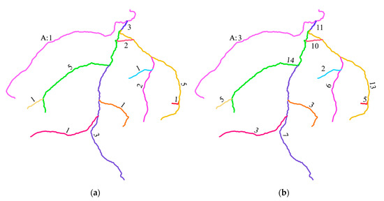
Figure 18.
The statistics of intersecting features: (a) NFIF values; (b) NSIF values.
Furthermore, unlike polyline data and polygon data, there is no similar intersecting or neighboring relationship for points in point data. Therefore, the proposed method is not suitable for point data. Converting points to polylines or polygons seems like a feasible approach to making it possible. For example, construct points to the Voronoi diagram. This will be further investigated in our future works.
5.3. The Watermark Uniqueness
The watermark uniqueness is one of the most important indexes in zero watermarking. It is determined by the characteristics of the data used to construct the watermark. A good zero watermarking algorithm needs to ensure that the watermarks constructed from different data are very different. To verify the watermark uniqueness of the proposed method, we selected six test data that are all administrative division maps, denoted Data 1–6, as shown in Figure 19. First, construct watermarks from the six test data using the proposed method. Then calculate NC values between the six watermarks and the watermark generated by the experimental data in Section 3.1, respectively. If the NC values are less than the threshold, it means that the method has good watermark uniqueness; otherwise, the method is not qualified. Finally, considering that the watermark length will affect the watermark uniqueness, we choose different watermark lengths for experiments: 32, 64, 128, and 256. Therefore, four groups of experimental results are produced, each with six NC values, as shown in Figure 20.
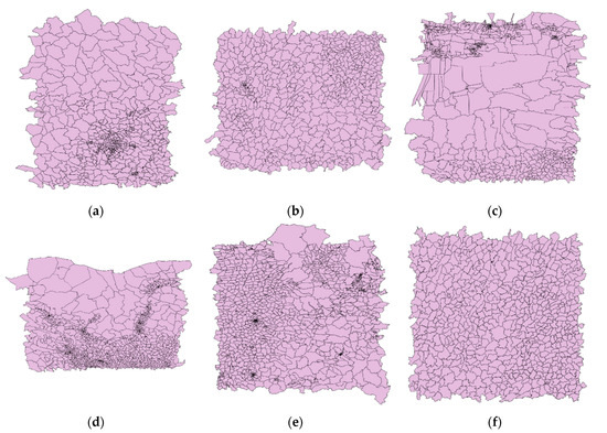
Figure 19.
The test data for the watermark uniqueness: (a) Data 1; (b) Data 2; (c) Data 3; (d) Data 4; (e) Data 5; (f) Data 6.
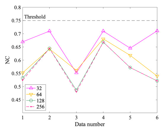
Figure 20.
The watermark uniqueness test with different watermark lengths.
It can be observed in Figure 20 that all the NC values are less than the threshold for the six test data under four different watermark lengths. And it roughly shows a trend that the longer the watermark length, the lower the NC value for the data. In detail, the maximum of the NC values is 0.71, and most of them are concentrated around 0.55 and 0.65, which are less than the threshold of 0.75. This proved that the proposed method meets the requirement of the watermark uniqueness.
6. Conclusions
In zero watermarking for vector geographic data, resisting attacks that cause significant distortion of the data is a challenging problem. The key is to find the characteristics that are not affected by data deformation. In this paper, two local characteristics are introduced: NFNF and NSNF, and they are quantified to the watermark bit and the watermark index, respectively. Among them, NSNF, the number of second-order neighboring features, is the first time introduced into the watermarking for vector geographic data in the state-of-the-art of watermarking research. Further, NFNS and NSNF make full use of the topological and statistical characteristics of the data, which are the foundation of the proposed method. Experimental results show that this method has good robustness and can completely resist attacks with significant distortion compared with other algorithms, such as non-uniform scaling, simplification, and projection transformation attacks. The proposal of this method is a new exploration in improving the robustness of zero watermarking for vector geographic data. Moreover, the combination of topological characteristics and statistical characteristics can provide some ideas for the future watermarking research. However, this method is not suitable for point data. Exploring the conversion methods of point data to polyline data and polygon data will be the focus of our future research.
Author Contributions
Conceptualization, Q.Z., N.R. and W.C.; methodology, Q.Z., N.R. and C.Z.; validation, Q.Z. and W.G.; formal analysis, Q.Z., W.G. and N.R.; writing—original draft preparation, Q.Z. and C.Z.; writing—review and editing, Q.Z., W.C. and C.Z.; visualization, Q.Z., W.C. and W.G.; supervision, N.R. and C.Z.; funding acquisition, C.Z., N.R. and Q.Z. All authors have read and agreed to the published version of the manuscript.
Funding
This research was funded by the National Natural Science Foundation of China under Grant 42071362, 41971338; the Natural Science Foundation of Jiangsu Province under Grant BK20191373; and the Graduate Research and Innovation Projects of Jiangsu Province under Grant KYCX20_1182.
Institutional Review Board Statement
Not applicable.
Informed Consent Statement
Not applicable.
Data Availability Statement
Not Applicable.
Conflicts of Interest
The authors declare no conflict of interest.
References
- Goodchild, M.F. Reimagining the history of GIS. Ann. GIS 2018, 24, 1–8. [Google Scholar] [CrossRef]
- Abubahia, A.; Cocea, M. Advancements in GIS map copyright protection schemes—A critical review. Multimed. Tools Appl. 2017, 76, 12205–12231. [Google Scholar] [CrossRef]
- Zhu, C. Research Progresses in Digital Watermarking and Encryption Control for Geographical Data. Acta Geod. Cartogr. Sin. 2017, 46, 1609–1619. [Google Scholar] [CrossRef]
- López, C. Watermarking of digital geospatial datasets: A review of technical, legal and copyright issues. Int. J. Geogr. Inf. Sci. 2002, 16, 589–607. [Google Scholar] [CrossRef]
- Peng, F.; Lin, Z.; Zhang, X.; Long, M. Reversible Data Hiding in Encrypted 2D Vector Graphics Based on Reversible Mapping Model for Real Numbers. IEEE Trans. Inf. Forensics Secur. 2019, 14, 2400–2411. [Google Scholar] [CrossRef]
- Hou, X.; Min, L.; Yang, H. A Reversible Watermarking Scheme for Vector Maps Based on Multilevel Histogram Modification. Symmetry 2018, 10, 397. [Google Scholar] [CrossRef]
- Wen, Q.; Sun, T.F.; Wang, S.X. Concept and Application of Zero-Watermark. Acta Electron. Sin. 2003, 31, 214–216. [Google Scholar]
- Liu, Y.; Yang, F.; Gao, K.; Dong, W.; Song, J. A zero-watermarking scheme with embedding timestamp in vector maps for Big Data computing. Cluster Comput. 2017, 20, 3667–3675. [Google Scholar] [CrossRef]
- Li, A.; Lin, B.; Chen, Y.; Lü, G. Study on copyright authentication of GIS vector data based on Zero-watermarking. Int. Arch. Photogramm. Remote Sens. Spat. Inf. Sci. 2008, XXXVIII, 1783–1786. [Google Scholar]
- Shih, F.Y. Digital Watermarking and Steganography: Fundamentals and Techniques, 2nd ed.; CRC Press: Boca Raton, FL, USA, 2017. [Google Scholar]
- Cox, I.J.; Miller, M.L.; Bloom, J.A.; Fridrich, J.; Kalker, T. Digital Watermarking and Steganography, 2nd ed.; Morgan Kaufmann Publishers: Burlington, MA, USA, 2008. [Google Scholar]
- Peng, Z.; Yue, M.; Wu, X.; Peng, Y. Blind watermarking scheme for polylines in vector geo-spatial data. Multimed. Tools Appl. 2015, 74, 11721–11739. [Google Scholar] [CrossRef]
- Abbas, T.A.; Jawad, M.J. Digital Vector Map Watermarking: Applications, Techniques and Attacks. Orient. J. Comput. Sci. Technol. 2013, 6, 333–339. [Google Scholar] [CrossRef]
- Sun, H.; Zhu, J.; Li, G.; Shi, Y. A zero-watermarking algorithm for vector map based on element coding. Geotech. Investig. Surv. 2012, 9, 54–57. [Google Scholar]
- Zhou, L.; Huang, Y.; Chen, Z.; Li, X. A Zero-watermarking Algorithm of SVG Vector Map Based on Stroke-width Characteristic. In Proceedings of the 2nd International Conference on Intelligent Computing and Cognitive Informatics, Singapore, 8–9 September 2015; Atlantis Press: Paris, France, 2015; pp. 34–37. [Google Scholar]
- Zhou, L.; Huang, Y.; Chen, Z.; Wu, L. A Zero-watermarking algorithm of SVG vector tiles. Sci. Surv. Mapp. 2016, 41, 132–135. [Google Scholar] [CrossRef]
- Zhou, L.; Chen, Z.; Wu, L.; Jiang, B. A zero-watermarking algorithm of map symbol library based on item characteristics. Sci. Surv. Mapp. 2017, 42, 137–142. [Google Scholar] [CrossRef]
- Zhang, Z.; Sun, S.; Wang, Y.; Zheng, K. Zero-watermarking algorithm for 2D vector map. Comput. Eng. Des. 2009, 30, 1473–1476. [Google Scholar] [CrossRef]
- Xi, X.; Zhang, X.; Liang, W.; Xin, Q.; Zhang, P. Dual Zero-Watermarking Scheme for Two-Dimensional Vector Map Based on Delaunay Triangle Mesh and Singular Value Decomposition. Appl. Sci. 2019, 9, 642. [Google Scholar] [CrossRef]
- Cao, L.; Men, C.; Sun, J. A double zero-watermarking algorithm for 2D vector maps. J. Harbin Eng. Univ. 2011, 32, 340–344. [Google Scholar]
- Du, Q.; Peng, F. A Zero-Watermark Algorithm with Real-Mean for 2D Engineering Graphic. In Proceedings of the 2008 International Symposium on Electronic Commerce and Security, Guangzhou, China, 3–5 August 2008; pp. 890–893. [Google Scholar]
- Zhao, H.; Du, S.; Zhang, D. Zero-watermark scheme for 2D vector drawings based on mapping. In Proceedings of the 2013 International Conference on Information Science and Cloud Computing Companion, ISCC-C 2013, Gunagzhou, China, 7–8 December 2014; pp. 601–605. [Google Scholar]
- Han, Z. Study on Lossless Digital Watermarking Algorithm for Vector Map based on Space Feature; China University of Petroleum: Beijing, China, 2017. [Google Scholar]
- Wang, X.; Huang, D.; Zhang, Z. A Robust Zero-Watermarking Algorithm for Vector Digital Maps Based on Statistical Characteristics. J. Softw. 2012, 7, 2349–2356. [Google Scholar] [CrossRef]
- Lyu, W.; Zhang, L. A zero-watermarking algorithm for vector data based on the distribution center. Eng. Surv. Mapp. 2017, 26, 50–53. [Google Scholar]
- Sun, Y.; Li, D. Vector Map Zero-Watermark Algorithm Based on Node Feature. Geogr. Geo-Inf. Sci. 2017, 33, 17–21. [Google Scholar] [CrossRef]
- Peng, Y.; Yue, M. A Zero-Watermarking Scheme for Vector Map Based on Feature Vertex Distance Ratio. J. Electr. Comput. Eng. 2015, 2015, 1–6. [Google Scholar] [CrossRef]
- Li, A.B.; Zhu, A.X. Copyright authentication of digital vector maps based on spatial autocorrelation indices. Earth Sci. Inform. 2019, 12, 629–639. [Google Scholar] [CrossRef]
- Sun, H.; Zhu, J.; Yin, P.; Shi, Y. Zero-Watermarking Algorithm Based on Feature Vertices of Vector Map and Blocking (in Chinese). Geogr. Geo-Inf. Sci. 2012, 28, 111–112. [Google Scholar]
- Liang, W.; Zhang, X.; Xi, X.; Zhang, P. A multiple watermarking algorithm for vector geographic data based on zero-watermarking and fragile watermarking. Zhongshan Daxue Xuebao/Acta Sci. Natralium Univ. Sunyatseni 2018, 57, 1–8. [Google Scholar] [CrossRef]
- Li, W.; Yan, H.; Wang, Z.; Zhang, L. A Zero-Watermarking Algorithm for Vector Linear Feature Data. J. Geomat. Sci. Technol. 2016, 33, 94–98. [Google Scholar]
- Fan, Y.; Chai, J.; Han, Z.; Tian, C. A Zero-Watermarking Algorithm Based on Minimum Quad-Tree Division and Feature Angle. Geomat. Spat. Inf. Technol. 2018, 41, 1–4. [Google Scholar]
- Zhou, Q.; Ren, N.; Zhu, C.; Zhu, A. Blind Digital Watermarking Algorithm against Projection Transformation for Vector Geographic Data. ISPRS Int. J. Geo-Inf. 2020, 9, 692. [Google Scholar] [CrossRef]
- Lin, Z.-X.; Peng, F.; Long, M. A Low-Distortion Reversible Watermarking for 2D Engineering Graphics Based on Region Nesting. IEEE Trans. Inf. Forensics Secur. 2018, 13, 2372–2382. [Google Scholar] [CrossRef]


Publisher’s Note: MDPI stays neutral with regard to jurisdictional claims in published maps and institutional affiliations. |
© 2021 by the authors. Licensee MDPI, Basel, Switzerland. This article is an open access article distributed under the terms and conditions of the Creative Commons Attribution (CC BY) license (http://creativecommons.org/licenses/by/4.0/).